1 Introduction

We begin by reviewing some elementary results that will be employed throughout this book and which will also serve to introduce notation.

1.1 Probability review

1.1.1 Random variables

A triple \((\Omega,\mathcal{A},\mathbb{P})\) is called a probability space. \(\Omega\) represents the sample space, the set of all possible individual outcomes of a random experiment. \(\mathcal{A}\) is a \(\sigma\)-field, a class of subsets of \(\Omega\) that is closed under complementation and countable unions, and such that \(\Omega\in\mathcal{A}.\) \(\mathcal{A}\) represents the collection of possible events (combinations of individual outcomes) that are assigned a probability by the probability measure \(\mathbb{P}.\) A random variable is a map \(X:\Omega\longrightarrow\mathbb{R}\) such that \(X^{-1}((-\infty,x])=\{\omega\in\Omega:X(\omega)\leq x\}\in\mathcal{A},\) \(\forall x\in\mathbb{R}\) (the set \(X^{-1}((-\infty,x])\) of possible outcomes of \(X\) is said to be measurable).

1.1.2 Cumulative distribution and probability density functions

The cumulative distribution function (cdf) of a random variable \(X\) is \(F(x):=\mathbb{P}[X\leq x].\) When an independent and identically distributed (iid) sample \(X_1,\ldots,X_n\) is given, the cdf can be estimated by the empirical distribution function (ecdf)

\[\begin{align} F_n(x)=\frac{1}{n}\sum_{i=1}^n1_{\{X_i\leq x\}}, \tag{1.1} \end{align}\]

where \(1_A:=\begin{cases}1,&A\text{ is true},\\0,&A\text{ is false}\end{cases}\) is an indicator function.²

Continuous random variables are characterized by either the cdf \(F\) or the probability density function (pdf) \(f=F',\) the latter representing the infinitesimal relative probability of \(X\) per unit length. We write \(X\sim F\) (or \(X\sim f\)) to denote that \(X\) has a cdf \(F\) (or a pdf \(f\)). If two random variables \(X\) and \(Y\) have the same distribution, we write \(X\stackrel{d}{=}Y.\)

1.1.3 Expectation

The expectation operator is constructed using the Riemann–Stieltjes “\(\,\mathrm{d}F(x)\)” integral.³ Hence, for \(X\sim F,\) the expectation of \(g(X)\) is

\[\begin{align*} \mathbb{E}[g(X)]:=&\,\int g(x)\,\mathrm{d}F(x)\\ =&\, \begin{cases} \displaystyle\int g(x)f(x)\,\mathrm{d}x,&\text{ if }X\text{ is continuous,}\\\displaystyle\sum_{\{x\in\mathbb{R}:\mathbb{P}[X=x]>0\}} g(x)\mathbb{P}[X=x],&\text{ if }X\text{ is discrete.} \end{cases} \end{align*}\]

Unless otherwise stated, the integration limits of any integral are \(\mathbb{R}\) or \(\mathbb{R}^p.\) The variance operator is defined as \(\mathbb{V}\mathrm{ar}[X]:=\mathbb{E}[(X-\mathbb{E}[X])^2].\)

1.1.4 Random vectors, marginals, and conditionals

We employ bold face to denote vectors, assumed to be column matrices, and matrices. A \(p\)-random vector is a map \(\mathbf{X}:\Omega\longrightarrow\mathbb{R}^p,\) \(\mathbf{X}(\omega):=(X_1(\omega),\ldots,X_p(\omega))^\top,\) such that each \(X_i\) is a random variable. The (joint) cdf of \(\mathbf{X}\) is \(F(\mathbf{x}):=\mathbb{P}[\mathbf{X}\leq \mathbf{x}]:=\mathbb{P}[X_1\leq x_1,\ldots,X_p\leq x_p]\) and, if \(\mathbf{X}\) is continuous, its (joint) pdf is \(f:=\frac{\partial^p}{\partial x_1\cdots\partial x_p}F.\)

The marginals of \(F\) and \(f\) are the cdfs and pdfs of \(X_i,\) \(i=1,\ldots,p,\) respectively. They are defined as

\[\begin{align*} F_{X_i}(x_i)&:=\mathbb{P}[X_i\leq x_i]=F(\infty,\ldots,\infty,x_i,\infty,\ldots,\infty),\\ f_{X_i}(x_i)&:=\frac{\partial}{\partial x_i}F_{X_i}(x_i)=\int_{\mathbb{R}^{p-1}} f(\mathbf{x})\,\mathrm{d}\mathbf{x}_{-i}, \end{align*}\]

where \(\mathbf{x}_{-i}:=(x_1,\ldots,x_{i-1},x_{i+1},\ldots,x_p)^\top.\) The definitions can be extended analogously to the marginals of the cdf and pdf of different subsets of \(\mathbf{X}.\)

The conditional cdf and pdf of \(X_1 \mid (X_2,\ldots,X_p)\) are defined, respectively, as

\[\begin{align*} F_{X_1\mid \mathbf{X}_{-1}=\mathbf{x}_{-1}}(x_1)&:=\mathbb{P}[X_1\leq x_1\mid \mathbf{X}_{-1}=\mathbf{x}_{-1}],\\ f_{X_1\mid \mathbf{X}_{-1}=\mathbf{x}_{-1}}(x_1)&:=\frac{f(\mathbf{x})}{f_{\mathbf{X}_{-1}}(\mathbf{x}_{-1})}. \end{align*}\]

The conditional expectation of \(Y \mid X\) is the following random variable⁴

\[\begin{align*} \mathbb{E}[Y\mid X]:=\int y \,\mathrm{d}F_{Y\mid X}(y\mid X). \end{align*}\]

The conditional variance of \(Y \mid X\) is defined as

\[\begin{align*} \mathbb{V}\mathrm{ar}[Y\mid X]:=\mathbb{E}[(Y-\mathbb{E}[Y\mid X])^2\mid X]=\mathbb{E}[Y^2\mid X]-\mathbb{E}[Y\mid X]^2. \end{align*}\]

Proposition 1.1 (Laws of total expectation and variance) Let \(X\) and \(Y\) be two random variables.

• Total expectation: if \(\mathbb{E}[|Y|]<\infty,\) then \(\mathbb{E}[Y]=\mathbb{E}[\mathbb{E}[Y \mid X]].\)
• Total variance: if \(\mathbb{E}[Y^2]<\infty,\) then \(\mathbb{V}\mathrm{ar}[Y]=\mathbb{E}[\mathbb{V}\mathrm{ar}[Y \mid X]]+\mathbb{V}\mathrm{ar}[\mathbb{E}[Y \mid X]].\)

Exercise 1.1 Prove the law of total variance from the law of total expectation.

Figure 1.1 graphically summarizes the concepts of joint, marginal, and conditional distributions within the context of a \(2\)-dimensional normal.

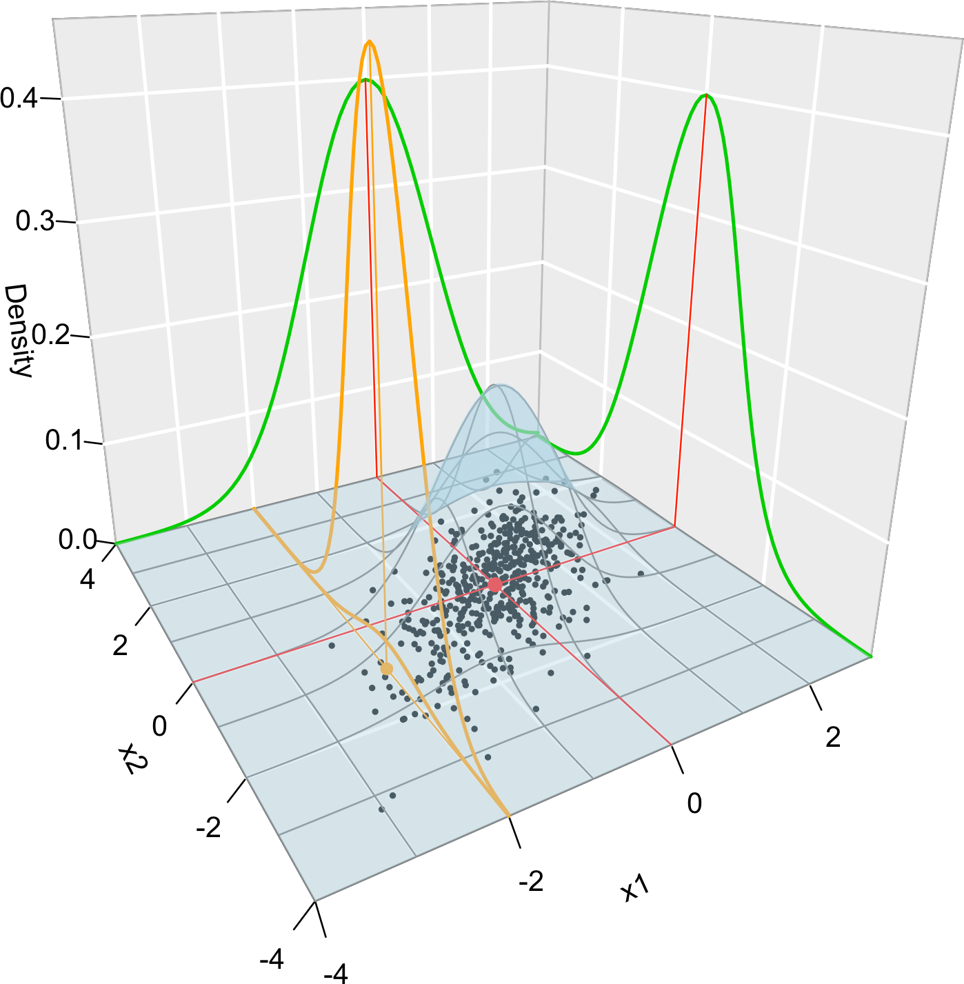
Figure 1.1: Visualization of the joint pdf (in blue), marginal pdfs (green), conditional pdf of \(X_2 \mid X_1=x_1\) (orange), expectation (red point), and conditional expectation \(\mathbb{E}\lbrack X_2 \mid X_1=x_1 \rbrack\) (orange point) of a \(2\)-dimensional normal. The conditioning point of \(X_1\) is \(x_1=-2.\) Note the different scales of the densities, as they have to integrate to one over different supports. Note how the conditional density (upper orange curve) is not the joint pdf \(f(x_1,x_2)\) (lower orange curve) with \(x_1=-2\) but its rescaling by \(\frac{1}{f_{X_1}(x_1)}.\) The parameters of the \(2\)-dimensional normal are \(\mu_1=\mu_2=0,\) \(\sigma_1=\sigma_2=1\) and \(\rho=0.75\) (see Exercise 1.9). \(500\) observations sampled from the distribution are shown in black.

Exercise 1.2 Consider the random vector \((X,Y)\) with joint pdf \[\begin{align*} f(x,y)=\begin{cases} y e^{-a x y},&x>0,\,y\in(0, b),\\ 0,&\text{else.} \end{cases} \end{align*}\]

1. Determine the value of \(b>0\) that makes \(f\) a valid pdf.
2. Compute \(\mathbb{E}[X]\) and \(\mathbb{E}[Y].\)
3. Verify the law of the total expectation.
4. Verify the law of the total variance.

Exercise 1.3 Consider the continuous random vector \((X_1,X_2)\) with joint pdf given by

\[\begin{align*} f(x_1,x_2)=\begin{cases} 2,&0<x_1<x_2<1,\\ 0,&\mathrm{else.} \end{cases} \end{align*}\]

1. Check that \(f\) is a proper pdf.
2. Obtain the joint cdf of \((X_1,X_2).\)
3. Obtain the marginal pdfs of \(X_1\) and \(X_2.\)
4. Obtain the marginal cdfs of \(X_1\) and \(X_2.\)
5. Obtain the conditional pdfs of \(X_1 \mid X_2=x_2\) and \(X_2 \mid X_1=x_1.\)

1.1.5 Variance-covariance matrix

For two random variables \(X_1\) and \(X_2,\) the covariance between them is defined as

\[\begin{align*} \mathrm{Cov}[X_1,X_2]:=\mathbb{E}[(X_1-\mathbb{E}[X_1])(X_2-\mathbb{E}[X_2])]=\mathbb{E}[X_1X_2]-\mathbb{E}[X_1]\mathbb{E}[X_2], \end{align*}\]

and the correlation between them, as

\[\begin{align*} \mathrm{Cor}[X_1,X_2]:=\frac{\mathrm{Cov}[X_1,X_2]}{\sqrt{\mathbb{V}\mathrm{ar}[X_1]\mathbb{V}\mathrm{ar}[X_2]}}. \end{align*}\]

The variance and the covariance are extended to a random vector \(\mathbf{X}=(X_1,\ldots,X_p)^\top\) by means of the so-called variance-covariance matrix:

\[\begin{align*} \mathbb{V}\mathrm{ar}[\mathbf{X}]:=&\,\mathbb{E}[(\mathbf{X}-\mathbb{E}[\mathbf{X}])(\mathbf{X}-\mathbb{E}[\mathbf{X}])^\top]\\ =&\,\mathbb{E}[\mathbf{X}\mathbf{X}^\top]-\mathbb{E}[\mathbf{X}]\mathbb{E}[\mathbf{X}]^\top\\ =&\,\begin{pmatrix} \mathbb{V}\mathrm{ar}[X_1] & \mathrm{Cov}[X_1,X_2] & \cdots & \mathrm{Cov}[X_1,X_p]\\ \mathrm{Cov}[X_2,X_1] & \mathbb{V}\mathrm{ar}[X_2] & \cdots & \mathrm{Cov}[X_2,X_p]\\ \vdots & \vdots & \ddots & \vdots \\ \mathrm{Cov}[X_p,X_1] & \mathrm{Cov}[X_p,X_2] & \cdots & \mathbb{V}\mathrm{ar}[X_p]\\ \end{pmatrix}, \end{align*}\]

where \(\mathbb{E}[\mathbf{X}]:=(\mathbb{E}[X_1],\ldots,\mathbb{E}[X_p])^\top\) is just the componentwise expectation. As in the univariate case, the expectation is a linear operator, which now means that

\[\begin{align} \mathbb{E}[\mathbf{A}\mathbf{X}+\mathbf{b}]=\mathbf{A}\mathbb{E}[\mathbf{X}]+\mathbf{b},\quad\text{for a $q\times p$ matrix } \mathbf{A}\text{ and }\mathbf{b}\in\mathbb{R}^q.\tag{1.2} \end{align}\]

It follows from (1.2) that

\[\begin{align} \mathbb{V}\mathrm{ar}[\mathbf{A}\mathbf{X}+\mathbf{b}]=\mathbf{A}\mathbb{V}\mathrm{ar}[\mathbf{X}]\mathbf{A}^\top,\quad\text{for a $q\times p$ matrix } \mathbf{A}\text{ and }\mathbf{b}\in\mathbb{R}^q.\tag{1.3} \end{align}\]

1.1.6 Inequalities

We conclude this section by reviewing some useful probabilistic inequalities.

Proposition 1.2 (Markov's inequality) Let \(X\) be a nonnegative random variable with \(\mathbb{E}[X]<\infty.\) Then

\[\begin{align*} \mathbb{P}[X\geq t]\leq\frac{\mathbb{E}[X]}{t}, \quad\forall t>0. \end{align*}\]

Proposition 1.3 (Chebyshev's inequality) Let \(X\) be a random variable with \(\mu=\mathbb{E}[X]\) and \(\sigma^2=\mathbb{V}\mathrm{ar}[X]<\infty.\) Then

\[\begin{align*} \mathbb{P}[|X-\mu|\geq t]\leq\frac{\sigma^2}{t^2},\quad \forall t>0. \end{align*}\]

Exercise 1.4 Prove Markov’s inequality using \(X=X1_{\{X\geq t\}}+X1_{\{X< t\}}.\)

Exercise 1.5 Prove Chebyshev’s inequality using Markov’s.

Remark. Chebyshev’s inequality gives a quick and handy way of computing confidence intervals for the values of any random variable \(X\) with finite variance:

\[\begin{align} \mathbb{P}[X\in(\mu-t\sigma, \mu+t\sigma)]\geq 1-\frac{1}{t^2},\quad \forall t>0.\tag{1.4} \end{align}\]

That is, for any \(t>0,\) the interval \((\mu-t\sigma, \mu+t\sigma)\) has, at least, a probability \(1-1/t^2\) of containing a random realization of \(X.\) The intervals are conservative, but extremely general. The table below gives the guaranteed coverage probability \(1-1/t^2\) for common values of \(t.\)

\(t\)	\(2\)	\(3\)	\(4\)	\(5\)	\(6\)
Guaranteed coverage	\(0.75\)	\(0.8889\)	\(0.9375\)	\(0.96\)	\(0.9722\)

Exercise 1.6 Prove (1.4) from Chebyshev’s inequality.

Proposition 1.4 (Cauchy–Schwarz inequality) Let \(X\) and \(Y\) such that \(\mathbb{E}[X^2]<\infty\) and \(\mathbb{E}[Y^2]<\infty.\) Then

\[\begin{align*} |\mathbb{E}[XY]|\leq\sqrt{\mathbb{E}[X^2]\mathbb{E}[Y^2]}. \end{align*}\]

Exercise 1.7 Prove Cauchy–Schwarz inequality “pulling a rabbit out of a hat”: consider the polynomial \(p(t)=\mathbb{E}[(tX+Y)^2]=At^2+2Bt+C\geq0,\) \(\forall t\in\mathbb{R}.\)

Exercise 1.8 Does \(\mathbb{E}[|XY|]\leq\sqrt{\mathbb{E}[X^2]\mathbb{E}[Y^2]}\) hold? Observe that, due to the next proposition, \(|\mathbb{E}[XY]|\leq \mathbb{E}[|XY|].\)

Proposition 1.5 (Jensen's inequality) If \(g\) is a convex function, then

\[\begin{align*} g(\mathbb{E}[X])\leq\mathbb{E}[g(X)]. \end{align*}\]

Example 1.1 Jensen’s inequality has interesting derivations. For example:

1. Take \(h=-g.\) Then \(h\) is a concave function and \(h(\mathbb{E}[X])\geq\mathbb{E}[h(X)].\)
2. Take \(g(x)=|x|^r\) for \(r\geq 1,\) which is a convex function. Then \(|\mathbb{E}[X]|^r\leq \mathbb{E}[|X|^r].\) If \(0<r<1,\) then \(g(x)=|x|^r\) is concave and \(|\mathbb{E}[X]|^r\geq \mathbb{E}[|X|^r].\)
3. Consider \(0<r\leq s.\) Then \(g(x)=|x|^{s/r}\) is convex (since \(s/r\geq 1\)) and \(g(\mathbb{E}[|X|^r])\leq \mathbb{E}[g(|X|^r)]=\mathbb{E}[|X|^s].\) As a consequence, \(\mathbb{E}[|X|^s]<\infty\implies\mathbb{E}[|X|^r]<\infty\) for \(0\leq r\leq s.\)⁵
4. The exponential (logarithm) function is convex (concave). Consequently, \(\exp(\mathbb{E}[X])\leq\mathbb{E}[\exp(X)]\) and \(\log(\mathbb{E}[|X|])\geq\mathbb{E}[\log(|X|)].\)

1.2 Facts about distributions

We will make use of certain parametric distributions. Some notation and facts are introduced as follows.

1.2.1 Normal distribution

The normal distribution with mean \(\mu\) and variance \(\sigma^2\) is denoted by \(\mathcal{N}(\mu,\sigma^2).\) Its pdf is \(\phi_\sigma(x-\mu):=\frac{1}{\sqrt{2\pi}\sigma}e^{-\frac{(x-\mu)^2}{2\sigma^2}},\) \(x\in\mathbb{R},\) and satisfies that \(\phi_\sigma(x-\mu)=\frac{1}{\sigma}\phi\left(\frac{x-\mu}{\sigma}\right)\) (if \(\sigma=1\) the dependence on \(\sigma\) is omitted). Its cdf is denoted by \(\Phi_\sigma(x-\mu).\) The upper \(\alpha\)-quantile of a \(\mathcal{N}(0,1)\) is denoted by \(z_\alpha,\) so it satisfies that \(z_\alpha=\Phi^{-1}(1-\alpha).\)⁶ The shortest interval that contains \(1-\alpha\) probability of a \(X\sim\mathcal{N}(\mu,\sigma^2)\) is \((\mu-z_{\alpha/2}\sigma,\mu+z_{\alpha/2}\sigma),\) i.e., \(\mathbb{P}[X\in(\mu\pm z_{\alpha/2}\sigma)]=1-\alpha.\) Some uncentered moments of \(X\sim\mathcal{N}(\mu,\sigma^2)\) are

\[\begin{align*} \mathbb{E}[X]&=\mu,\\ \mathbb{E}[X^2]&=\mu^2+\sigma^2,\\ \mathbb{E}[X^3]&=\mu^3+3\mu\sigma^2,\\ \mathbb{E}[X^4]&=\mu^4+6\mu^2\sigma^2+3\sigma^4. \end{align*}\]

Remark. It is interesting to compare the length of \((\mu\pm z_{\alpha/2}\sigma)\) for \(\alpha=1/t^2\) with the one in (1.4), as this gives direct insight into how larger the Chebyshev confidence interval (1.4) is when \(X\sim\mathcal{N}(\mu,\sigma^2).\) The table below gives the length increment factor \(t/z_{(0.5/t^2)}\) of the Chebyshev confidence interval.

\(t\)	\(2\)	\(3\)	\(4\)	\(5\)	\(6\)
Guaranteed coverage	\(0.75\)	\(0.8889\)	\(0.9375\)	\(0.96\)	\(0.9722\)
Increment factor	\(1.7386\)	\(1.883\)	\(2.1474\)	\(2.4346\)	\(2.7268\)

Balancing between the guaranteed coverage and increment factor, it seems reasonable to define the “\(3\sigma\)-rule” for any random variable as: “almost \(90\%\) of the values of a random variable \(X\) lie on \((\mu-3\sigma,\mu+3\sigma),\) if \(\mathbb{E}[X]=\mu\) and \(\mathbb{V}\mathrm{ar}[X]=\sigma^2<\infty\)”.

The multivariate normal is represented by \(\mathcal{N}_p(\boldsymbol{\mu},\boldsymbol{\Sigma}),\) where \(\boldsymbol{\mu}\) is a \(p\)-vector and \(\boldsymbol{\Sigma}\) is a \(p\times p\) symmetric and positive definite matrix. The pdf of a \(\mathcal{N}(\boldsymbol{\mu},\boldsymbol{\Sigma})\) is \(\phi_{\boldsymbol{\Sigma}}(\mathbf{x}-\boldsymbol{\mu}):=\frac{1}{(2\pi)^{p/2}|\boldsymbol{\Sigma}|^{1/2}}e^{-\frac{1}{2}(\mathbf{x}-\boldsymbol{\mu})^\top\boldsymbol{\Sigma}^{-1}(\mathbf{x}-\boldsymbol{\mu})}\) and satisfies that \(\phi_{\boldsymbol{\Sigma}}(\mathbf{x}-\boldsymbol{\mu})=|\boldsymbol{\Sigma}|^{-1/2}\phi\big(\boldsymbol{\Sigma}^{-1/2}(\mathbf{x}-\boldsymbol{\mu})\big)\) (if \(\boldsymbol{\Sigma}=\mathbf{I},\) the dependence on \(\boldsymbol{\Sigma}\) is omitted). The multivariate normal has an appealing linear property that stems from (1.2) and (1.3):

\[\begin{align} \mathbf{A}\mathcal{N}_p(\boldsymbol\mu,\boldsymbol\Sigma)+\mathbf{b}\stackrel{d}{=}\mathcal{N}_q(\mathbf{A}\boldsymbol\mu+\mathbf{b},\mathbf{A}\boldsymbol\Sigma\mathbf{A}^\top).\tag{1.5} \end{align}\]

Exercise 1.9 The pdf of a bivariate normal (\(p=2,\) see Figure 1.1) can be also expressed as

\[\begin{align} &\phi(x_1,x_2;\mu_1,\mu_2,\sigma_1^2,\sigma_2^2,\rho):=\frac{1}{2\pi\sigma_1\sigma_2\sqrt{1-\rho^2}}\tag{1.6}\\ &\,\times\!\exp\left\{\!-\frac{1}{2(1-\rho^2)}\!\left[\frac{(x_1-\mu_1)^2}{\sigma_1^2}+\frac{(x_2-\mu_2)^2}{\sigma_2^2}-\frac{2\rho(x_1-\mu_1)(x_2-\mu_2)}{\sigma_1\sigma_2}\right]\!\right\}\!,\nonumber \end{align}\]

where \(\mu_1,\mu_2\in\mathbb{R},\) \(\sigma_1,\sigma_2>0,\) and \(-1<\rho<1.\) The parametrization uses \(\boldsymbol{\mu}=(\mu_1,\mu_2)^\top\) and \(\boldsymbol{\Sigma}=(\sigma_1^2,\rho\sigma_1\sigma_2;\rho\sigma_1\sigma_2,\sigma_2^2).\)⁷

1. Derive the pdf of \(X_1\): \(\phi(x_1;\mu_1,\sigma_1^2).\)
2. Derive the pdf of \(X_1 \mid X_2=x_2\): \(\phi\big(x_1;\mu_1+\rho\frac{\sigma_1}{\sigma_2}(x_2-\mu_2),(1-\rho^2)\sigma_1^2\big).\)
3. Derive \(\mathbb{E}[X_1 \mid X_2=x_2]\) and \(\mathbb{V}\mathrm{ar}[X_1 \mid X_2=x_2].\)

1.2.2 Other distributions

• The lognormal distribution is denoted by \(\mathcal{LN}(\mu,\sigma^2)\) and is such that \(\mathcal{LN}(\mu,\sigma^2)\stackrel{d}{=}\exp(\mathcal{N}(\mu,\sigma^2)).\) Its pdf is \(f(x;\mu,\sigma)=\frac{1}{x}\phi_\sigma(\log x-\log\mu)=\frac{1}{\sqrt{2\pi}\sigma x}e^{-\frac{(\log x-\log\mu)^2}{2\sigma^2}},\) \(x>0.\) Note that \(\mathbb{E}[\mathcal{LN}(\mu,\sigma^2)]=e^{\mu+\frac{\sigma^2}{2}}\) and \(\mathbb{V}\mathrm{ar}[\mathcal{LN}(\mu,\sigma^2)]=\big(e^{\sigma^2}-1\big)e^{2\mu+\sigma^2}.\)

• The exponential distribution is denoted by \(\mathrm{Exp}(\lambda)\) and has pdf \(f(x;\lambda)=\lambda e^{-\lambda x},\) \(\lambda,x>0.\)

• The gamma distribution is denoted by \(\Gamma(a,p)\) and has pdf \(f(x;a,p)=\frac{a^p}{\Gamma(p)} x^{p-1}e^{-a x},\) \(a,p,x>0,\) where \(\Gamma(p)=\int_0^\infty x^{p-1}e^{-ax}\,\mathrm{d}x.\) The parameter \(a\) is the rate and \(p\) is the shape. It is known that \(\mathbb{E}[\Gamma(a,p)]=\frac{p}{a}\) and \(\mathbb{V}\mathrm{ar}[\Gamma(a,p)]=\frac{p}{a^2}.\)

• The inverse gamma distribution, \(\mathrm{IG}(a,p)\stackrel{d}{=}\Gamma(a,p)^{-1},\) has pdf \(f(x;a,p)=\frac{a^p}{\Gamma(p)} x^{-p-1}e^{-\frac{a}{x}},\) \(a,p,x>0.\) It is known that \(\mathbb{E}[\mathrm{IG}(a,p)]=\frac{a}{p-1}\) and \(\mathbb{V}\mathrm{ar}[\mathrm{IG}(a,p)]=\frac{a^2}{(p-1)^2(p-2)}.\)

• The binomial distribution is denoted by \(\mathrm{B}(n,p).\) Recall that \(\mathbb{E}[\mathrm{B}(n,p)]=np\) and \(\mathbb{V}\mathrm{ar}[\mathrm{B}(n,p)]=np(1-p).\) A \(\mathrm{B}(1,p)\) is a Bernoulli distribution, denoted by \(\mathrm{Ber}(p).\)

• The beta distribution is denoted by \(\beta(a,b)\) and its pdf is \(f(x;a,b)=\frac{1}{\beta(a,b)}x^{a-1}(1-x)^{1-b},\) \(0<x<1,\) where \(\beta(a,b)=\frac{\Gamma(a)\Gamma(b)}{\Gamma(a+b)}.\) When \(a=b=1,\) the uniform distribution \(\mathcal{U}(0,1)\) arises.

• The Poisson distribution is denoted by \(\mathrm{Pois}(\lambda)\) and has probability mass function \(\mathbb{P}[X=x]=\frac{\lambda^x e^{-\lambda}}{x!},\) \(x=0,1,2,\ldots\) Recall that \(\mathbb{E}[\mathrm{Pois}(\lambda)]=\mathbb{V}\mathrm{ar}[\mathrm{Pois}(\lambda)]=\lambda.\)

1.3 Stochastic convergence review

Let \(X_n\) be a sequence of random variables defined in a common probability space \((\Omega,\mathcal{A},\mathbb{P}).\) The four most common types of convergence of \(X_n\) to a random variable in \((\Omega,\mathcal{A},\mathbb{P})\) are the following.

Definition 1.1 (Convergence in distribution) \(X_n\) converges in distribution to \(X,\) written \(X_n\stackrel{d}{\longrightarrow}X,\) if \(\lim_{n\to\infty}F_n(x)=F(x)\) for all \(x\) for which \(F\) is continuous, where \(X_n\sim F_n\) and \(X\sim F.\)

“Convergence in distribution” is also referred to as weak convergence. Proposition 1.6 justifies this terminology.

Definition 1.2 (Convergence in probability) \(X_n\) converges in probability to \(X,\) written \(X_n\stackrel{\mathbb{P}}{\longrightarrow}X,\) if \(\lim_{n\to\infty}\mathbb{P}[|X_n-X|>\varepsilon]=0,\) \(\forall \varepsilon>0.\)

Definition 1.3 (Convergence almost surely) \(X_n\) converges almost surely (as) to \(X,\) written \(X_n\stackrel{\mathrm{as}}{\longrightarrow}X,\) if \(\mathbb{P}[\{\omega\in\Omega:\lim_{n\to\infty}X_n(\omega)=X(\omega)\}]=1.\)

Definition 1.4 (Convergence in \(r\)-mean) For \(r\geq1,\) \(X_n\) converges in \(r\)-mean to \(X,\) written \(X_n\stackrel{r}{\longrightarrow}X,\) if \(\lim_{n\to\infty}\mathbb{E}[|X_n-X|^r]=0.\)

Remark. The previous definitions can be extended to a sequence of \(p\)-random vectors \(\mathbf{X}_n.\) For Definitions 1.2 and 1.4, replace \(|\cdot|\) with the Euclidean norm \(||\cdot||.\) Alternatively, Definition 1.2 can be extended marginally: \(\mathbf{X}_n\stackrel{\mathbb{P}}{\longrightarrow}\mathbf{X}\,:\!\iff X_{j,n}\stackrel{\mathbb{P}}{\longrightarrow}X_j,\) \(\forall j=1,\ldots,p.\) For Definition 1.1, replace \(F_n\) and \(F\) by the joint cdfs of \(\mathbf{X}_n\) and \(\mathbf{X},\) respectively.⁸ Definition 1.3 also extends marginally.

The \(2\)-mean convergence plays a remarkable role in defining a consistent estimator \(\hat\theta_n=T(X_1,\ldots,X_n)\) of a parameter \(\theta.\) We say that the estimator is consistent if its Mean Squared Error (MSE),

\[\begin{align*} \mathrm{MSE}[\hat\theta_n]:\!&=\mathbb{E}[(\hat\theta_n-\theta)^2]\\ &=(\mathbb{E}[\hat\theta_n]-\theta)^2+\mathbb{V}\mathrm{ar}[\hat\theta_n]\\ &=:\mathrm{Bias}[\hat\theta_n]^2+\mathbb{V}\mathrm{ar}[\hat\theta_n], \end{align*}\]

goes to zero as \(n\to\infty.\) Equivalently written, if \(\hat\theta_n\stackrel{2}{\longrightarrow}\theta.\)

If \(X_n\stackrel{d,\mathbb{P},r,\mathrm{as}}{\longrightarrow} X\) and \(X\) is a degenerate random variable such that \(\mathbb{P}[X=c]=1,\) \(c\in\mathbb{R},\) then we write \(X_n\stackrel{d,\mathbb{P},r,\mathrm{as}}{\longrightarrow} c\) (the list-notation \(\stackrel{d,\mathbb{P},r,\mathrm{as}}{\longrightarrow}\) is used here and henceforth to condense several different convergence results in the same line).

The relations between the types of convergences are conveniently summarized in the following proposition.

Proposition 1.6 Let \(X_n\) be a sequence of random variables and \(X\) a random variable. Then the following implication diagram is satisfied:

\[\begin{align*} \begin{array}{rcl} X_n\stackrel{r}{\longrightarrow}X \quad\implies & X_n\stackrel{\mathbb{P}}{\longrightarrow}X & \impliedby\quad X_n\stackrel{\mathrm{as}}{\longrightarrow}X\\ & \Downarrow & \\ & X_n\stackrel{d}{\longrightarrow}X & \end{array} \end{align*}\]

Also, if \(s\geq r\geq 1,\) then \(X_n\stackrel{s}{\longrightarrow}X\implies X_n\stackrel{r}{\longrightarrow}X.\)

None of the converses holds in general. However, there are some notable exceptions:

1. If \(X_n\stackrel{d}{\longrightarrow}c,\) then \(X_n\stackrel{\mathbb{P}}{\longrightarrow}c,\) \(c\in\mathbb{R}.\)
2. If \(\forall\varepsilon>0,\) \(\lim_{n\to\infty}\sum_n\mathbb{P}[|X_n-X|>\varepsilon]<\infty\) (implies⁹ \(X_n\stackrel{\mathbb{P}}{\longrightarrow}X\)), then \(X_n\stackrel{\mathrm{as}}{\longrightarrow}X.\)
3. If \(X_n\stackrel{\mathbb{P}}{\longrightarrow}X\) and \(\mathbb{P}[|X_n|\leq M]=1,\) \(\forall n\in\mathbb{N}\) and \(M>0,\)¹⁰ then \(X_n\stackrel{r}{\longrightarrow}X\) for \(r\geq1.\)
4. If \(S_n=\sum_{i=1}^nX_i\) with \(X_1,\ldots,X_n\) iid, then \(S_n\stackrel{\mathbb{P}}{\longrightarrow}S\iff S_n\stackrel{\mathrm{as}}{\longrightarrow}S.\)

The weak Law of Large Numbers (LLN) and its strong version are the two most representative results of convergence in probability and almost surely.

Theorem 1.1 (Weak and strong LLN) Let \(X_n\) be an iid sequence with \(\mathbb{E}[X_i]=\mu,\) \(i\geq1.\) Then: \(\frac{1}{n}\sum_{i=1}^nX_i\stackrel{\mathbb{P},\,\mathrm{as}}{\longrightarrow}\mu.\)

The cornerstone limit result in probability is the Central Limit Theorem (CLT). One of its simpler versions has the following form.

Theorem 1.2 (CLT) Let \(X_n\) be a sequence of iid random variables with \(\mathbb{E}[X_i]=\mu\) and \(\mathbb{V}\mathrm{ar}[X_i]=\sigma^2<\infty,\) \(i\in\mathbb{N}.\) Then:

\[\begin{align*} \frac{\sqrt{n}(\bar{X}-\mu)}{\sigma}\stackrel{d}{\longrightarrow}\mathcal{N}(0,1). \end{align*}\]

We will later use the following CLT for random variables that are independent but not identically distributed due to its easy-to-check moment conditions.

Theorem 1.3 (Lyapunov's CLT) Let \(X_n\) be a sequence of independent random variables with \(\mathbb{E}[X_i]=\mu_i\) and \(\mathbb{V}\mathrm{ar}[X_i]=\sigma_i^2<\infty,\) \(i\in\mathbb{N},\) and such that for some \(\delta>0\)

\[\begin{align*} \frac{1}{s_n^{2+\delta}}\sum_{i=1}^n\mathbb{E}\left[|X_i-\mu_i|^{2+\delta}\right]\longrightarrow0\text{ as }n\to\infty, \end{align*}\]

with \(s_n^2=\sum_{i=1}^n\sigma^2_i.\) Then:

\[\begin{align*} \frac{1}{s_n}\sum_{i=1}^n(X_i-\mu_i)\stackrel{d}{\longrightarrow}\mathcal{N}(0,1). \end{align*}\]

Finally, the following results will be useful (\(^\top\) denotes transposition). In particular, Slutsky’s theorem allows mixing the LLNs and the CLT with additions and products.

Theorem 1.4 (Cramér–Wold device) Let \(\mathbf{X}_n\) be a sequence of \(p\)-dimensional random vectors. Then:

\[\begin{align*} \mathbf{X}_n\stackrel{d}{\longrightarrow}\mathbf{X}\iff \mathbf{c}^\top\mathbf{X}_n\stackrel{d}{\longrightarrow}\mathbf{c}^\top\mathbf{X},\quad \forall \mathbf{c}\in\mathbb{R}^p. \end{align*}\]

Theorem 1.5 (Continuous mapping theorem) If \(\mathbf{X}_n\stackrel{d,\,\mathbb{P},\,\mathrm{as}}{\longrightarrow}\mathbf{X},\) then

\[\begin{align*} g(\mathbf{X}_n)\stackrel{d,\,\mathbb{P},\,\mathrm{as}}{\longrightarrow}g(\mathbf{X}) \end{align*}\]

for any continuous function \(g.\)

Theorem 1.6 (Slutsky's theorem) Let \(X_n\) and \(Y_n\) be sequences of random variables and \(c\in\mathbb{R}.\) Then:

1. If \(X_n\stackrel{d}{\longrightarrow}X\) and \(Y_n\stackrel{\mathbb{P}}{\longrightarrow} c,\) then \(X_nY_n\stackrel{d}{\longrightarrow}cX.\)
2. If \(X_n\stackrel{d}{\longrightarrow}X\) and \(Y_n\stackrel{\mathbb{P}}{\longrightarrow} c,\) \(c\neq0,\) then \(\frac{X_n}{Y_n}\stackrel{d}{\longrightarrow}\frac{X}{c}.\)
3. If \(X_n\stackrel{d}{\longrightarrow}X\) and \(Y_n\stackrel{\mathbb{P}}{\longrightarrow} c,\) then \(X_n+Y_n\stackrel{d}{\longrightarrow}X+c.\)

Theorem 1.7 (Limit algebra for \((\mathbb{P},\,r,\,\mathrm{as})\)-convergence) Let \(X_n\) and \(Y_n\) be sequences of random variables, and \(a_n\to a\) and \(b_n\to b\) two sequences.

1. If \(X_n\stackrel{\mathbb{P},\,r,\,\mathrm{as}}{\longrightarrow}X\) and \(Y_n\stackrel{\mathbb{P},\,r,\,\mathrm{as}}{\longrightarrow}Y,\) then \(a_nX_n+b_nY_n\stackrel{\mathbb{P},\,r,\,\mathrm{as}}{\longrightarrow}aX+bY.\)
2. If \(X_n\stackrel{\mathbb{P},\,\mathrm{as}}{\longrightarrow}X\) and \(Y_n\stackrel{\mathbb{P},\,\mathrm{as}}{\longrightarrow}Y,\) then \(X_nY_n\stackrel{\mathbb{P},\,\mathrm{as}}{\longrightarrow}XY.\)

Remark. Recall the absence of the analogous results for convergence in distribution. In general, there are no such results!

• Particularly, it is false that, in general, \(X_n\stackrel{d}{\longrightarrow}X\) and \(Y_n\stackrel{d}{\longrightarrow}Y\) imply \(X_n+Y_n\stackrel{d}{\longrightarrow}X+Y\) or \(X_nY_n\stackrel{d}{\longrightarrow}XY\).
• It is true, however, that \((X_n,Y_n)\stackrel{d}{\longrightarrow}(X,Y)\) (a much stronger premise) implies both \(X_n+Y_n\stackrel{d}{\longrightarrow}X+Y\) and \(X_nY_n\stackrel{d}{\longrightarrow}XY,\) as Theorem 1.5 indicates. Note that \(X_n+Y_n\stackrel{d}{\longrightarrow}X+Y\) is also implied by \((X_n,Y_n)\stackrel{d}{\longrightarrow}(X,Y)\) by Theorem 1.4 with \(\mathbf{c}=(1,1)^\top.\)
• Consequently, it is also true that, under independence of \(X_n\) and \(Y_n,\) \(X_n\stackrel{d}{\longrightarrow}X\) and \(Y_n\stackrel{d}{\longrightarrow}Y\) imply \(X_n+Y_n\stackrel{d}{\longrightarrow}X+Y\) and \(X_nY_n\stackrel{d}{\longrightarrow}XY\)

Theorem 1.8 (Delta method) If \(\sqrt{n}(X_n-\mu)\stackrel{d}{\longrightarrow}\mathcal{N}(0,\sigma^2),\) then

\[\begin{align*} \sqrt{n}(g(X_n)-g(\mu))\stackrel{d}{\longrightarrow}\mathcal{N}\left(0,(g'(\mu))^2\sigma^2\right) \end{align*}\]

for any function \(g\) that is differentiable at \(\mu\) and such that \(g'(\mu)\neq0.\)

Example 1.2 It is well known that, given a parametric density \(f_\theta\) with parameter \(\theta\in\Theta\) and iid \(X_1,\ldots,X_n\sim f_\theta,\) then the Maximum Likelihood (ML) estimator \(\hat\theta_{\mathrm{ML}}:=\arg\max_{\theta\in\Theta}\sum_{i=1}^n\log f_\theta(X_i)\) (the parameter that maximizes the “probability” of the data based on the model) converges to a normal under certain regularity conditions:

\[\begin{align*} \sqrt{n}(\hat\theta_{\mathrm{ML}}-\theta)\stackrel{d}{\longrightarrow}\mathcal{N}\left(0,I(\theta)^{-1}\right), \end{align*}\]

where \(I(\theta):=-\mathbb{E}_\theta\left[\frac{\partial^2\log f_\theta(x)}{\partial\theta^2}\right]\) is known as the Fisher information. Then, it is satisfied that

\[\begin{align*} \sqrt{n}(g(\hat\theta_{\mathrm{ML}})-g(\theta))\stackrel{d}{\longrightarrow}\mathcal{N}\left(0,(g'(\theta))^2I(\theta)^{-1}\right). \end{align*}\]

Note that, had we applied the continuous mapping theorem for \(g,\) we would have obtained a different result:

\[\begin{align*} g(\sqrt{n}(\hat\theta_{\mathrm{ML}}-\theta))\stackrel{d}{\longrightarrow}g\left(\mathcal{N}\left(0,I(\theta)^{-1}\right)\right). \end{align*}\]

Exercise 1.10 Let’s dig further into the differences between the delta method and the continuous mapping theorem when applied to \(\sqrt{n}(X_n-\mu)\stackrel{d}{\longrightarrow}\mathcal{N}(0,\sigma^2)\):

1. For which functions \(g\) are the statements \(\sqrt{n}(g(X_n)-g(\mu))\stackrel{d}{\longrightarrow}\mathcal{N}(0,(g'(\mu))^2\sigma^2)\) and \(g(\sqrt{n}(X_n-\mu))\stackrel{d}{\longrightarrow}g(\mathcal{N}(0,\sigma^2))\) equivalent?
2. Take \(g(x)=e^x.\) What two results do you obtain with the delta method and the continuous mapping theorem when applied to \(\sqrt{n}\bar X \stackrel{d}{\longrightarrow}\mathcal{N}(0,\sigma^2)\)?

1.4 \(O_\mathbb{P}\) and \(o_\mathbb{P}\) notation

1.4.1 Deterministic versions

In computer science the \(O\) notation is used to measure the complexity of algorithms. For example, when an algorithm is \(O(n^2),\) it is said that it is quadratic in time and we know that it is going to take on the order of \(n^2\) operations to process an input of size \(n.\) We do not care about the specific amount of computations; rather, we focus on the big picture by looking for an upper bound for the sequence of computation times in terms of \(n.\) This upper bound disregards constants. For example, the dot product between two vectors of size \(n\) is an \(O(n)\) operation, although it takes \(n\) multiplications and \(n-1\) sums, hence \(2n-1\) operations. In essence, the \(O\) notation allows us to trade precision for simplicity.

In mathematical analysis, \(O\)-related notation is mostly used to bound sequences that shrink to zero. This is the use we will be concerned about. The technicalities are the same, but the use of the notation is slightly different.

Definition 1.5 (Big-\(O\)) Given two strictly positive sequences \(a_n\) and \(b_n,\)

\[\begin{align*} a_n=O(b_n)\,:\!\iff \limsup_{n\to\infty}\frac{a_n}{b_n}\leq C,\text{ for a }C>0. \end{align*}\]

If \(a_n=O(b_n),\) then we say that \(a_n\) is big-\(O\) of \(b_n.\) To indicate that \(a_n\) is bounded, we write \(a_n=O(1).\)¹¹

Definition 1.6 (Little-\(o\)) Given two strictly positive sequences \(a_n\) and \(b_n,\)

\[\begin{align*} a_n=o(b_n)\,:\!\iff \lim_{n\to\infty}\frac{a_n}{b_n}=0. \end{align*}\]

If \(a_n=o(b_n),\) then we say that \(a_n\) is little-\(o\) of \(b_n.\) To indicate that \(a_n\to0,\) we write \(a_n=o(1).\)

Remark. An immediate but important consequence of the big-\(O\) and little-\(o\) definitions is that

\[\begin{align} a_n=O(b_n)\!\iff \frac{a_n}{b_n}=O(1) \text{ and } a_n=o(b_n)\!\iff \frac{a_n}{b_n}=o(1). \tag{1.7} \end{align}\]

Exercise 1.11 Show the following statements by directly applying the previous definitions.

1. \(n^{-2}=o(n^{-1}).\)
2. \(\log n=O(n).\)
3. \(n^{-1}=o((\log n)^{-1}).\)
4. \(n^{-4/5}=o(n^{-2/3}).\)
5. \(3\sin(n)=O(1).\)
6. \(n^{-2}-n^{-3}+n^{-1}=O(n^{-1}).\)
7. \(n^{-2}-n^{-3}=o(n^{-1/2}).\)

The interpretation of these two definitions is simple:¹²

• \(a_n=O(b_n)\) means that \(a_n\) is “not larger than” \(b_n\) asymptotically. If \(a_n,b_n\to0,\) then it means that \(a_n\) “decreases as fast or faster” than \(b_n.\)
• \(a_n=o(b_n)\) means that \(a_n\) is “smaller than” \(b_n\) asymptotically. If \(a_n,b_n\to0,\) then it means that \(a_n\) “decreases faster” than \(b_n.\)

Obviously, little-\(o\) implies big-\(O\) (take any \(C>0\) in Definition 1.5). Playing with limits we can get a list of useful facts.

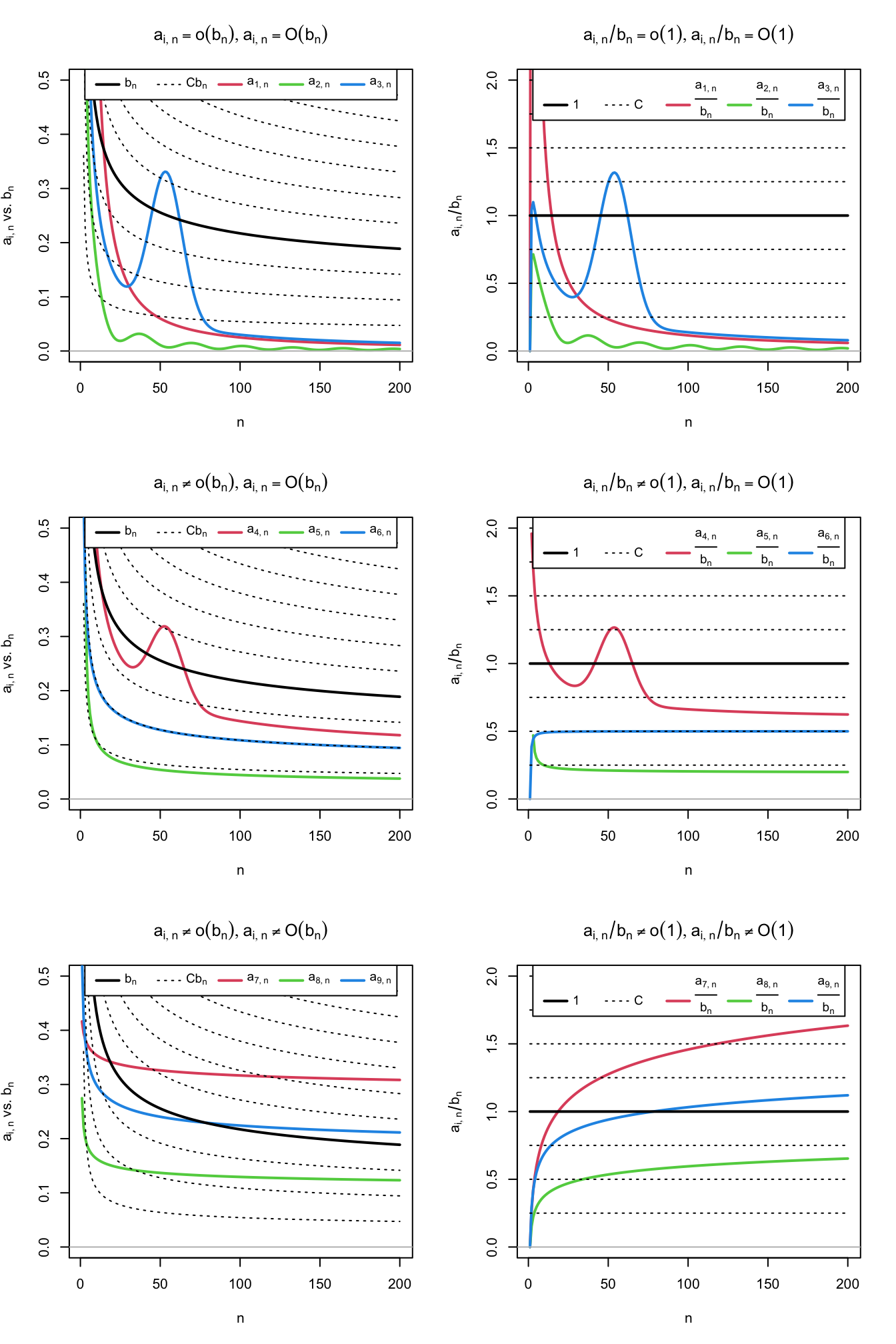
Figure 1.2: Differences and similarities between little-\(o\) and big-\(O,\) illustrated for the dominating sequence \(b_n=1/\log(n)\) (black solid curve) and sequences \(a_{i,n},\) \(i=1,\ldots,9\) (colored curves). The dashed lines represent the sequences \(Cb_n,\) for a grid of constants \(C.\) The plots on the left column compare \(a_{i,n}\) against \(b_n,\) whereas the right column plots show the equivalent view in terms of the ratios \(a_{i,n}/b_n\) (recall (1.7)). Sequences \(a_{1,n}=2 / n + 50 / n^2,\) \(a_{2,n}=(\sin(n/5) + 2) / n^{5/4},\) and \(a_{3,n}=3(1 + 5 \exp(-(n - 55.5)^2 / 200)) / n\) are \(o(b_n)\) (hence also \(O(b_n)\)). Sequences \(a_{4,n}=(2\log_{10}(n)((n + 3) / (2n)))^{-1} + a_{3,n}/2,\) \(a_{5,n}=(4\log_2(n/2))^{-1},\) and \(a_{6,n}=(\log(n^2 + n))^{-1}\) are \(O(b_n),\) but not \(o(b_n).\) Finally, sequences \(a_{7,n}=\log(5n + 3)^{-1/4}/2,\) \(a_{8,n}=(4\log(\log(10n + 2)))^{-1},\) and \(a_{9,n}=(2\log(\log(n^2 + 10n + 2)))^{-1}\) are not \(O(b_n)\) (hence neither \(o(b_n)\)).

Proposition 1.7 Consider two strictly positive sequences \(a_n,b_n\to0.\) The following properties hold:

1. \(kO(a_n)=O(a_n),\) \(ko(a_n)=o(a_n),\) \(k\in\mathbb{R}.\)
2. \(o(a_n)+o(b_n)=o(a_n+b_n),\) \(O(a_n)+O(b_n)=O(a_n+b_n).\)
3. \(o(a_n)o(b_n)=o(a_nb_n),\) \(O(a_n)O(b_n)=O(a_nb_n).\)
4. \(o(a_n)+O(b_n)=O(a_n+b_n),\) \(o(a_n)O(b_n)=o(a_nb_n).\)
5. \(o(1)O(a_n)=o(a_n).\)
6. \(a_n^r=o(a_n^s),\) for \(r>s\geq 0.\)
7. \(a_nb_n=o(a_n+b_n).\)
8. \((a_n+b_n)^k=O(a_n^k+b_n^k).\)

The last result is a consequence of a useful inequality.

Lemma 1.1 (\(C_p\) inequality) Given \(a,b\in\mathbb{R}\) and \(p>0,\)

\[\begin{align*} |a+b|^p\leq C_p(|a|^p+|b|^p), \quad C_p=\begin{cases} 1,&p\leq1,\\ 2^{p-1},&p>1. \end{cases} \end{align*}\]

Exercise 1.12 Illustrate the properties of Proposition 1.7 considering \(a_n=n^{-1}\) and \(b_n=n^{-1/2}.\)

1.4.2 Stochastic versions

The previous notation is purely deterministic. Let’s add some stochastic flavor by establishing the stochastic analogue of little-\(o.\)

Definition 1.7 (Little-\(o_\mathbb{P}\)) Given a strictly positive sequence \(a_n\) and a sequence of random variables \(X_n,\)

\[\begin{align*} X_n=o_\mathbb{P}(a_n)\,:\!\iff& \frac{|X_n|}{a_n}\stackrel{\mathbb{P}}{\longrightarrow}0 \\ \iff& \lim_{n\to\infty}\mathbb{P}\left[\frac{|X_n|}{a_n}>\varepsilon\right]=0,\;\forall\varepsilon>0. \end{align*}\]

If \(X_n=o_\mathbb{P}(a_n),\) then we say that \(X_n\) is little-\(o_\mathbb{P}\) of \(a_n.\) To indicate that \(X_n\stackrel{\mathbb{P}}{\longrightarrow}0,\) we write \(X_n=o_\mathbb{P}(1).\)

Therefore, little-\(o_\mathbb{P}\) allows us to easily quantify the speed at which a sequence of random variables converges to zero in probability.

Example 1.3 Let \(Y_n=o_\mathbb{P}\big(n^{-1/2}\big)\) and \(Z_n=o_\mathbb{P}(n^{-1}).\) Then \(Z_n\) converges faster to zero in probability than \(Y_n.\) To visualize this, recall that \(X_n=o_\mathbb{P}(a_n)\) and that limit definitions entail that

\[\begin{align*} \forall\varepsilon,\delta>0,\,\exists \,n_0=n_0(\varepsilon,\delta)\in\mathbb{N}:\forall n\geq n_0(\varepsilon,\delta),\, \mathbb{P}\left[|X_n|>a_n\varepsilon\right]<\delta. \end{align*}\]

Therefore, for fixed \(\varepsilon,\delta>0\) and a fixed \(n\geq\max(n_{0,Y},n_{0,Z}),\) then \(\mathbb{P}\left[Y_n\in\big(-n^{-1/2}\varepsilon,n^{-1/2}\varepsilon\big)\right]>1-\delta\) and \(\mathbb{P}\left[Z_n\in(-n^{-1}\varepsilon,n^{-1}\varepsilon)\right]>1-\delta,\) but the latter interval is much shorter, hence \(Z_n\) is forced to be more tightly concentrated about \(0.\)

Big-\(O_\mathbb{P}\) allows us to bound a sequence of random variables in probability, in the sense that we can state that the probability of being above an arbitrarily large threshold \(C\) converges to zero. As with its deterministic versions \(o\) and \(O,\) a little-\(o_\mathbb{P}\) is more restrictive than a big-\(O_\mathbb{P}\), and the former implies the latter.

Definition 1.8 (Big-\(O_\mathbb{P}\)) Given a strictly positive sequence \(a_n\) and a sequence of random variables \(X_n,\)

\[\begin{align*} X_n=O_\mathbb{P}(a_n)\,:\!\iff&\forall\varepsilon>0,\,\exists\,C_\varepsilon>0,\,n_0(\varepsilon)\in\mathbb{N}:\\ &\forall n\geq n_0(\varepsilon),\, \mathbb{P}\left[\frac{|X_n|}{a_n}>C_\varepsilon\right]<\varepsilon\\ \iff& \lim_{C\to\infty}\limsup_{n\to\infty}\mathbb{P}\left[\frac{|X_n|}{a_n}>C\right]=0. \end{align*}\]

If \(X_n=O_\mathbb{P}(a_n),\) then we say that \(X_n\) is big-\(O_\mathbb{P}\) of \(a_n.\)

Remark. An immediate but important consequence of the big-\(O_\mathbb{P}\) and little-\(o_\mathbb{P}\) definitions is that

\[\begin{align} X_n=O_\mathbb{P}(a_n)\!\iff \frac{X_n}{a_n}=O_\mathbb{P}(1) \text{ and } X_n=o_\mathbb{P}(a_n)\!\iff \frac{X_n}{a_n}=o_\mathbb{P}(1). \tag{1.8} \end{align}\]

Example 1.4 Any sequence of random variables such that \(X_n=X\) for all \(n\geq 1,\) with \(X\) any random variable, is trivially \(X_n=O_\mathbb{P}(1).\) Indeed, it is satisfied that \(\lim_{C\to\infty}\limsup_{n\to\infty}\mathbb{P}\left[\frac{|X_n|}{1}>C\right]=\lim_{C\to\infty}\mathbb{P}[|X_n|>C]=0.\)

Example 1.5 Chebyshev’s inequality entails that \(\mathbb{P}[|X_n-\mathbb{E}[X_n]|\geq t]\leq \mathbb{V}\mathrm{ar}[X_n]/t^2,\) \(\forall t>0.\) Setting \(\varepsilon:=\mathbb{V}\mathrm{ar}[X_n]/t^2\) and \(C_\varepsilon:=1/\sqrt{\varepsilon},\) then \(\mathbb{P}\left[|X_n-\mathbb{E}[X_n]|\geq \sqrt{\mathbb{V}\mathrm{ar}[X_n]}C_\varepsilon\right]\leq \varepsilon.\) Therefore,

\[\begin{align} X_n-\mathbb{E}[X_n]=O_\mathbb{P}\left(\sqrt{\mathbb{V}\mathrm{ar}[X_n]}\right).\tag{1.9} \end{align}\]

This is a very useful result, as it gives an efficient way of deriving the big-\(O_\mathbb{P}\) form of a sequence of random variables \(X_n\) with finite variances.

An application of Example 1.5 shows that \(X_n=O_\mathbb{P}(n^{-1/2})\) for \(X_n\stackrel{d}{=}\mathcal{N}(0,1/n).\) The nature of this statement and its relation with little-\(o_\mathbb{P}\) is visualized with Figure 1.3, which shows a particular realization \(X_n(\omega)\) of the sequence of random variables.

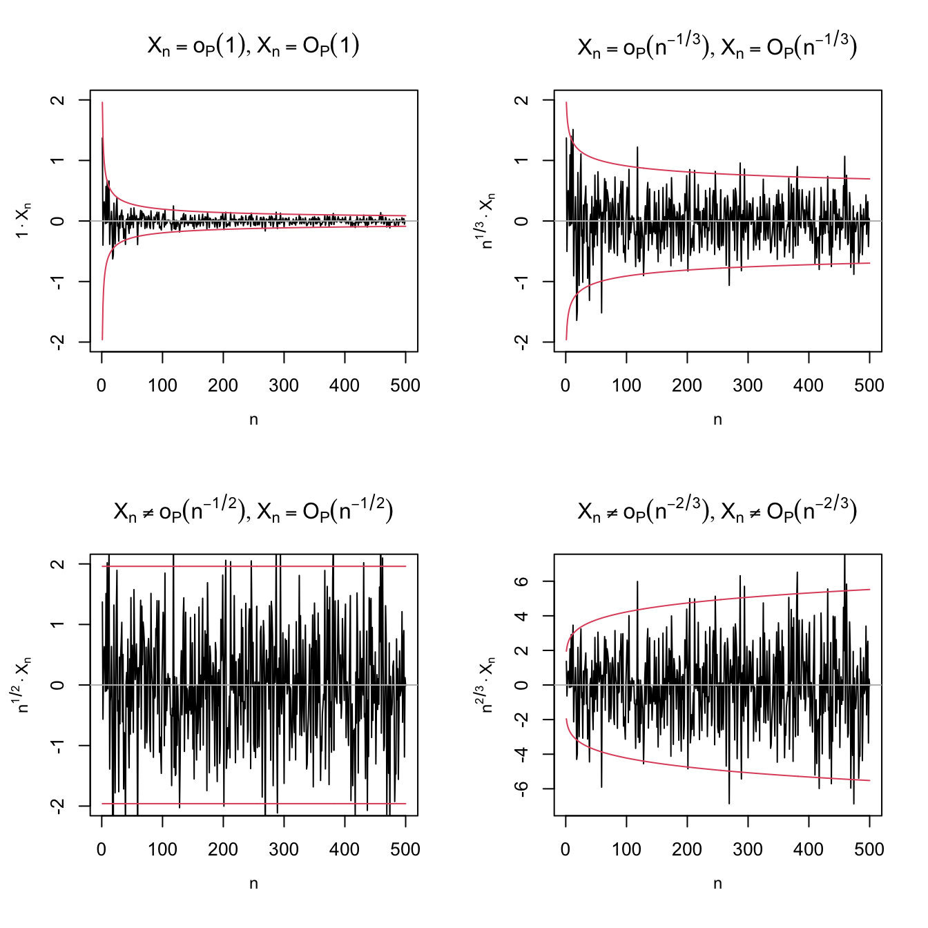
Figure 1.3: Differences and similarities between little-\(o_\mathbb{P}\) and big-\(O_\mathbb{P},\) illustrated for the sequence of random variables \(X_n\stackrel{d}{=}\mathcal{N}(0,1/n).\) Since \(X_n\stackrel{\mathbb{P}}{\longrightarrow}0,\) \(X_n=o_\mathbb{P}(1),\) as evidenced in the upper left plot. The next plots check if \(X_n=o_\mathbb{P}(a_n)\) by evaluating if \(X_n/a_n\stackrel{\mathbb{P}}{\longrightarrow}0\) (recall (1.8)), for \(a_n=n^{-1/3},n^{-1/2},n^{-2/3}.\) Clearly, \(X_n=o_\mathbb{P}(n^{-1/3})\) (\(n^{1/3}X_n\stackrel{\mathbb{P}}{\longrightarrow}0\)) but \(X_n\neq o_\mathbb{P}(n^{-1/2})\) (\(n^{1/2}X_n\stackrel{\mathbb{P}}{\longrightarrow}\mathcal{N}(0,1)\)) and \(X_n\neq o_\mathbb{P}(n^{-2/3})\) (\(n^{2/3}X_n\) diverges). In the first three cases, \(X_n=O_\mathbb{P}(a_n);\) the fourth is \(X_n\neq O_\mathbb{P}(n^{-2/3}),\) \(n^{2/3}X_n\) is not bounded in probability. The red lines represent the \(95\%\) confidence intervals \(\left(-z_{0.025}/(a_n\sqrt{n}),z_{0.025}/(a_n\sqrt{n})\right)\) of the random variable \(X_n/a_n,\) and help evaluating graphically the convergence in probability towards zero.

Exercise 1.13 As illustrated in Figure 1.3, prove that it is actually true that:

1. \(X_n\stackrel{\mathbb{P}}{\longrightarrow}0.\)
2. \(n^{1/3}X_n\stackrel{\mathbb{P}}{\longrightarrow}0.\)
3. \(n^{1/2}X_n\stackrel{\mathbb{P}}{\longrightarrow}\mathcal{N}(0,1).\)

Exercise 1.14 Prove that if \(X_n\stackrel{d}{\longrightarrow}X,\) then \(X_n=O_\mathbb{P}(1).\) Hint: use the double-limit definition and note that \(X=O_\mathbb{P}(1).\)

Example 1.6 (Example 1.18 in DasGupta (2008)) Suppose that \(a_n(X_n-c_n)\stackrel{d}{\longrightarrow}X\) for deterministic sequences \(a_n\) and \(c_n\) such that \(c_n\to c.\) Then, if \(a_n\to\infty,\) \(X_n-c=o_\mathbb{P}(1).\) The argument is simple:

\[\begin{align*} X_n-c&=X_n-c_n+c_n-c\\ &=\frac{1}{a_n}a_n(X_n-c_n)+o(1)\\ &=\frac{1}{a_n}O_\mathbb{P}(1)+o(1). \end{align*}\]

Exercise 1.15 Using the previous example, derive the weak law of large numbers as a consequence of the CLT, both for id and non-id independent random variables.

Proposition 1.8 Consider two strictly positive sequences \(a_n,b_n\to 0.\) The following properties hold:

1. \(o_\mathbb{P}(a_n)=O_\mathbb{P}(a_n)\) (little-\(o_\mathbb{P}\) implies big-\(O_\mathbb{P}\)).
2. \(o(1)=o_\mathbb{P}(1),\) \(O(1)=O_\mathbb{P}(1)\) (deterministic implies probabilistic).
3. \(kO_\mathbb{P}(a_n)=O_\mathbb{P}(a_n),\) \(ko_\mathbb{P}(a_n)=o_\mathbb{P}(a_n),\) \(k\in\mathbb{R}.\)
4. \(o_\mathbb{P}(a_n)+o_\mathbb{P}(b_n)=o_\mathbb{P}(a_n+b_n),\) \(O_\mathbb{P}(a_n)+O_\mathbb{P}(b_n)=O_\mathbb{P}(a_n+b_n).\)
5. \(o_\mathbb{P}(a_n)o_\mathbb{P}(b_n)=o_\mathbb{P}(a_nb_n),\) \(O_\mathbb{P}(a_n)O_\mathbb{P}(b_n)=O_\mathbb{P}(a_nb_n).\)
6. \(o_\mathbb{P}(a_n)+O_\mathbb{P}(b_n)=O_\mathbb{P}(a_n+b_n),\) \(o_\mathbb{P}(a_n)O_\mathbb{P}(b_n)=o_\mathbb{P}(a_nb_n).\)
7. \(o_\mathbb{P}(1)O_\mathbb{P}(a_n)=o_\mathbb{P}(a_n).\)
8. \((1+o_\mathbb{P}(1))^{-1}=O_\mathbb{P}(1).\)

Example 1.7 Example 1.5 allows us to obtain the \(O_\mathbb{P}\)-part of a sequence of random variables \(X_n\) with finite variances using (1.9). As a result of ii and iv in Proposition 1.8, we can also further simplify the coarse-grained description of \(X_n\) as

\[\begin{align*} X_n&=O(\mathbb{E}[X_n])+O_\mathbb{P}\left(\sqrt{\mathbb{V}\mathrm{ar}[X_n]}\right)\\ &=O_\mathbb{P}\left(\mathbb{E}[X_n]+\sqrt{\mathbb{V}\mathrm{ar}[X_n]}\right). \end{align*}\]

Exercise 1.16 Consider the following sequences of random variables:

1. \(X_n\stackrel{d}{=}\Gamma(n+1,2n)-2.\)
2. \(X_n\stackrel{d}{=}\mathrm{B}(n,1/n)-1.\)
3. \(X_n\stackrel{d}{=}\mathcal{LN}(0,n^{-1})-\exp((2n)^{-1}).\) Hint: Use that \(e^x=1+x+o(x)\) for \(x\to0.\)

For each \(X_n,\) obtain, if possible, two different positive sequences \(a_n,b_n\to0\) such that:

1. \(X_n=o_\mathbb{P}(a_n).\)
2. \(X_n\neq o_\mathbb{P}(b_n),\) \(X_n=O_\mathbb{P}(b_n).\)

Use (1.9) and check your results by performing an analogous analysis to that in Figure 1.3.

1.5 Review of basic analytical tools

We will make use of the following well-known analytical results.

Theorem 1.9 (Mean value theorem) Let \(f:[a,b]\longrightarrow\mathbb{R}\) be a continuous function and differentiable in \((a,b).\) Then there exists \(c\in(a,b)\) such that \(f(b)-f(a)=f'(c)(b-a).\)

Theorem 1.10 (Integral mean value theorem) Let \(f:[a,b]\longrightarrow\mathbb{R}\) be a continuous function over \((a,b).\) Then there exists \(c\in(a,b)\) such that \(\int_a^b f(x)\,\mathrm{d}x=f(c)(b-a).\)

Theorem 1.11 (Taylor's theorem) Let \(f:\mathbb{R}\longrightarrow\mathbb{R}\) and \(x\in\mathbb{R}.\) Assume that \(f\) has \(p\) continuous derivatives in an interval \((x-\delta,x+\delta)\) for a \(\delta>0.\) Then, for any \(|h|<\delta,\)

\[\begin{align*} f(x+h)=\sum_{j=0}^p\frac{f^{(j)}(x)}{j!}h^j+R_n,\quad R_n=o(h^p). \end{align*}\]

Remark. The remainder \(R_n\) depends on \(x\in\mathbb{R}.\) Explicit control of \(R_n\) is possible if \(f\) is further assumed to be \((p+1)\)-times differentiable in \((x-\delta,x+\delta).\) In that case, \(R_n=\frac{f^{(p+1)}(\xi_x)}{(p+1)!}h^{p+1}=o(h^p)\) for a certain \(\xi_x\in(x-\delta,x+\delta).\) Then, if \(f^{(p+1)}\) is bounded in \((x-\delta,x+\delta),\) \(\sup_{y\in(x-\delta,x+\delta)}\frac{R_n}{h^p}\to0,\) i.e., the remainder is \(o(h^p)\) uniformly in \((x-\delta,x+\delta).\) The remainder can also be put in an integral form that provides further control of the error term.

Theorem 1.12 (Dominated Convergence Theorem; DCT) Let \(f_n:S\subset\mathbb{R}\longrightarrow\mathbb{R}\) be a sequence of Lebesgue measurable functions such that \(\lim_{n\to\infty}f_n(x)=f(x)\) and \(|f_n(x)|\leq g(x),\) \(\forall x\in S\) and \(\forall n\in\mathbb{N},\) where \(\int_S |g(x)|\,\mathrm{d}x<\infty.\) Then

\[\begin{align*} \lim_{n\to\infty}\int_S f_n(x)\,\mathrm{d}x=\int_S f(x)\,\mathrm{d}x<\infty. \end{align*}\]

Remark. Note that if \(S\) is bounded and \(|f_n(x)|\leq M,\) \(\forall x\in S\) and \(\forall n\in\mathbb{N},\) then limit interchangeability with integral is always possible.

1.6 Why Nonparametric Statistics?

The aim of statistical inference is to use data to infer an unknown quantity. In the game of inference, there is usually a trade-off between efficiency and generality, and this trade-off is controlled by the strength of assumptions that are made on the data-generating process.

Parametric inference favors efficiency. Given a model (a strong assumption on the data-generating process), parametric inference delivers a set of methods (point estimation, confidence intervals, hypothesis testing, etc) tailored for such a model. All of these methods are the most efficient inferential procedures if the model matches the reality, in other words, if the data-generating process truly satisfies the assumptions. Otherwise the methods may be inconsistent.

Nonparametric inference favors generality. Given a set of minimal and weak assumptions (e.g., certain smoothness of a density or existence of moments of a random variable), it provides inferential methods that are consistent for broad situations, in exchange for losing efficiency for small or moderate sample sizes. Broadly speaking, a statistical technique qualifies as “nonparametric” if it does not rely on parametric assumptions, these typically having a finite-dimensional nature.¹³

Hence, for any specific data generation process there is a parametric method that dominates its nonparametric counterpart in efficiency. But knowledge of the data generation process is rarely the case in practice. That is the appeal of a nonparametric method: it will perform adequately no matter what the data generation process is. For that reason, nonparametric methods are useful:

1. When we have no clue on what could be a good parametric model.
2. For creating goodness-of-fit tests employed to validate parametric models.

The following example aims to illustrate the first advantage, the most useful in practice.

Example 1.8 Assume we have a sample \(X_1,\ldots,X_n\) from a random variable \(X\) and we want to estimate its distribution function \(F.\) Without any assumption, we know that the ecdf in (1.1) is an estimate for \(F(x)=\mathbb{P}[X\leq x].\) It is indeed a nonparametric estimate for \(F.\) Its expectation and variance are

\[\begin{align*} \mathbb{E}[F_n(x)]=F(x),\quad \mathbb{V}\mathrm{ar}[F_n(x)]=\frac{F(x)(1-F(x))}{n}. \end{align*}\]

From the squared bias and variance, we can get the MSE:

\[\begin{align*} \mathrm{MSE}[F_n(x)]=\frac{F(x)(1-F(x))}{n}. \end{align*}\]

Assume now that \(X\sim\mathrm{Exp}(\lambda).\) By maximum likelihood, it is possible to estimate \(\lambda\) as \(\hat \lambda_\mathrm{ML}={\bar X}^{-1}.\) Then, we have the following estimate for \(F(x)\):

\[\begin{align} F(x;\hat\lambda_\mathrm{ML})=1-e^{-\hat\lambda_\mathrm{ML} x}. \tag{1.10} \end{align}\]

Obtaining the exact MSE for (1.10) is not so simple, even if it is easy to prove that \(\hat\lambda_\mathrm{ML}\sim \mathrm{IG}(\lambda^{-1},n).\) Approximations are possible using Exercise 1.2. However, the MSE can be easily approximated by Monte Carlo.

What happens when the data is generated from an \(\mathrm{Exp}(\lambda)\)? Then (1.10) uniformly dominates (1.1) in performance. But, even for small deviations from \(\mathrm{Exp}(\lambda)\) given by \(\Gamma(\lambda, p),\) \(p\neq 1,\) the parametric estimator (1.10) shows major problems in terms of bias, while the performance of the nonparametric estimator (1.1) is completely unaltered. The animation in Figure 1.4 illustrates precisely this behavior.

Figure 1.4: A simplified example of parametric and nonparametric estimation. The objective is to estimate the distribution function \(F\) of a random variable. The data is generated from a \(\Gamma(\lambda,p).\) The parametric method assumes that \(p=1,\) that is, that the data comes from a \(\mathrm{Exp}(\lambda).\) The nonparametric method does not assume anything on the data generation process. The left plot shows the true distribution function and ten estimates of each method from samples of size \(n.\) The right plot shows the MSE of each method on estimating \(F(x).\) Application available here.

References

DasGupta, A. 2008. Asymptotic Theory of Statistics and Probability. Springer Texts in Statistics. New York: Springer. https://doi.org/10.1007/978-0-387-75971-5.

---

2. Inspiration for (1.1) comes from realizing that \(F(x)=\mathbb{E}[1_{\{X\leq x\}}].\)↩︎

3. See Riemann–Stieltjes integral.↩︎

4. Recall that the \(X\)-part of \(\mathbb{E}[Y \mid X]\) is random. However, \(\mathbb{E}[Y \mid X=x]\) is deterministic.↩︎

5. “Finite moments of higher order imply finite moments of lower order”.↩︎

6. A particular useful value for computing confidence intervals is \(z_{0.05/2}=z_{0.025}\approx 1.96\approx 2.\)↩︎

7. Note that this is an immediate parametrization of a \(2\times2\) covariance matrix. The parametrization becomes cumbersome when \(p>2.\)↩︎

8. Which is actually very different from a marginal extension!↩︎

9. Intuitively: if convergence in probability is fast enough, then we have almost sure convergence.↩︎

10. “Uniformly bounded random variables”.↩︎

11. For a deterministic sequence \(a_n,\) \(\limsup_{n\to\infty}a_n:=\lim_{n\to\infty}\left(\sup_{k\geq n}a_k\right)\) is the largest limit of the subsequences of \(a_n.\) It can be defined even if \(\lim_{n\to\infty}a_n\) does not exist (e.g., in trigonometric functions). If \(\lim_{n\to\infty}a_n\) exists, as in most of the common usages of the big-\(O\) notation, then \(\limsup_{n\to\infty}a_n=\lim_{n\to\infty}a_n.\)↩︎

12. For further intuition, we can regard \(a_n\) and \(b_n\) as two vehicles moving towards “zero”, a far away destination, with \(n\) indexing the time. The faster vehicle is the one that approaches zero more quickly. If \(a_n=O(b_n),\) then \(a_n\) is as fast or equal to \(b_n.\) If \(a_n=o(b_n),\) then \(a_n\) is strictly faster than \(b_n.\) The comparison is asymptotic, meaning that you focus on what happens on the long run (large \(n\)), disregarding initial differences. In this simplified example, \(\mathrm{plane}_n=O(\mathrm{car}_n)\) and \(\mathrm{car}_n=o(\mathrm{bike}_n)\), despite the fact that initially the car is faster than the plane and the bike can also be faster than the car.↩︎

13. For example, the exact two-sided \(t\)-test for the mean of a random variable \(X,\) i.e., the test \(H_0:\mu=\mu_0\) vs. \(H_1:\mu\neq\mu_0,\) assumes that \(X\sim\mathcal{N}(\mu,\sigma^2).\) This is an assumption indexed by the two parameters \((\mu,\sigma^2)\in\mathbb{R}\times\mathbb{R}^+.\)↩︎