2 Kernel density estimation I

A random variable $X$ is completely characterized by its cdf. Hence, an estimation of the cdf yields estimates for different characteristics of $X$ as side-products by plugging, in these characteristics, the ecdf $F_n$ instead of the $F.$ For example,¹⁴ the mean $\mu=\mathbb{E}[X]=\int x\,\mathrm{d}F(x)$ can be estimated by $\int x \,\mathrm{d}F_n(x)=\frac{1}{n}\sum_{i=1}^n X_i=\bar X.$

Despite their usefulness and many advantages, cdfs are hard to visualize and interpret, a consequence of their cumulative-based definition.

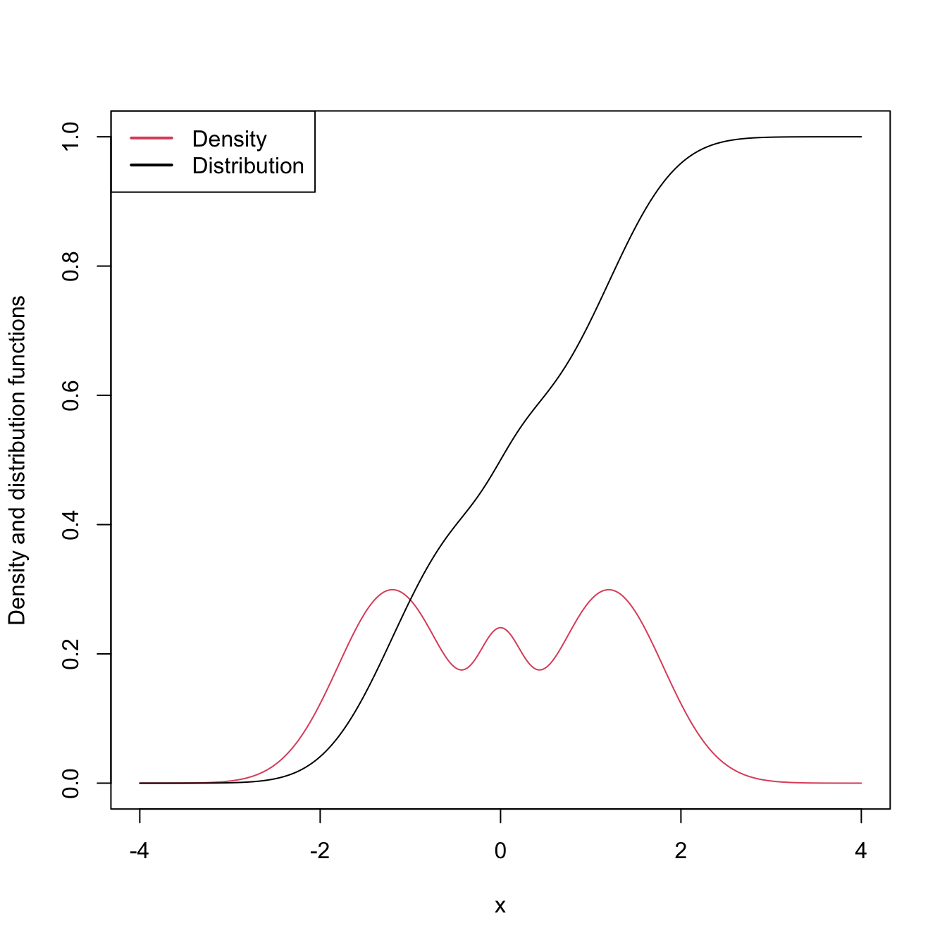
$The pdf and cdf of a mixture of three normals. The pdf yields better insights into the structure of the continuous random variable $X$ than the cdf does.$

Figure 2.1: The pdf and cdf of a mixture of three normals. The pdf yields better insights into the structure of the continuous random variable $X$ than the cdf does.

Densities, on the other hand, are easy to visualize and interpret, making them ideal tools for data exploration of continuous random variables. They provide immediate graphical information about the highest-density regions, modes, and shape of the support of $X.$ In addition, densities also completely characterize continuous random variables. Yet, even though a pdf follows from a cdf by the relation $f=F',$ density estimation does not follow immediately from the ecdf $F_n,$ since this function is not differentiable.¹⁵ Hence the need for specific procedures for estimating $f$ that we will see in this chapter.

2.1 Histograms

2.1.1 Histogram

The simplest method to estimate a density $f$ from an iid sample $X_1,\ldots,X_n$ is the histogram. From an analytical point of view, the idea is to aggregate the data in intervals of the form $[x_0,x_0+h)$ and then use their relative frequency to approximate the density at $x\in[x_0,x_0+h),$ $f(x),$ by the estimate of¹⁶

\[\begin{align*} f(x_0)&=F'(x_0)\\ &=\lim_{h\to0^+}\frac{F(x_0+h)-F(x_0)}{h}\\ &=\lim_{h\to0^+}\frac{\mathbb{P}[x_0<X< x_0+h]}{h}. \end{align*}\]

More precisely, given an origin $t_0$ and a bandwidth $h>0,$ the histogram builds a piecewise constant function in the intervals $\{B_k:=[t_{k},t_{k+1}):t_k=t_0+hk,k\in\mathbb{Z}\}$ by counting the number of sample points inside each of them. These constant-length intervals are also called bins. The fact that they are of constant length $h$ is important: we can easily standardize the counts on any bin by $h$ in order to have relative frequencies per length¹⁷ in the bins. The histogram at a point $x$ is defined as

\[\begin{align} \hat{f}_\mathrm{H}(x;t_0,h):=\frac{1}{nh}\sum_{i=1}^n1_{\{X_i\in B_k:x\in B_k\}}. \tag{2.1} \end{align}\]

Equivalently, if we denote the number of observations $X_1,\ldots,X_n$ in $B_k$ as $v_k,$ then the histogram can be written as

\[\begin{align*} \hat{f}_\mathrm{H}(x;t_0,h)=\frac{v_k}{nh},\quad\text{ if }x\in B_k\text{ for a certain }k\in\mathbb{Z}. \end{align*}\]

The computation of histograms is straightforward in R. As an example, we consider the old-but-gold faithful dataset. This dataset contains the duration of the eruption and the waiting time between eruptions for the Old Faithful geyser in Yellowstone National Park (USA).

# The faithful dataset is included in R
head(faithful)
##   eruptions waiting
## 1     3.600      79
## 2     1.800      54
## 3     3.333      74
## 4     2.283      62
## 5     4.533      85
## 6     2.883      55

# Duration of eruption
faith_eruptions <- faithful$eruptions

# Default histogram: automatically chosen bins and absolute frequencies!
histo <- hist(faith_eruptions)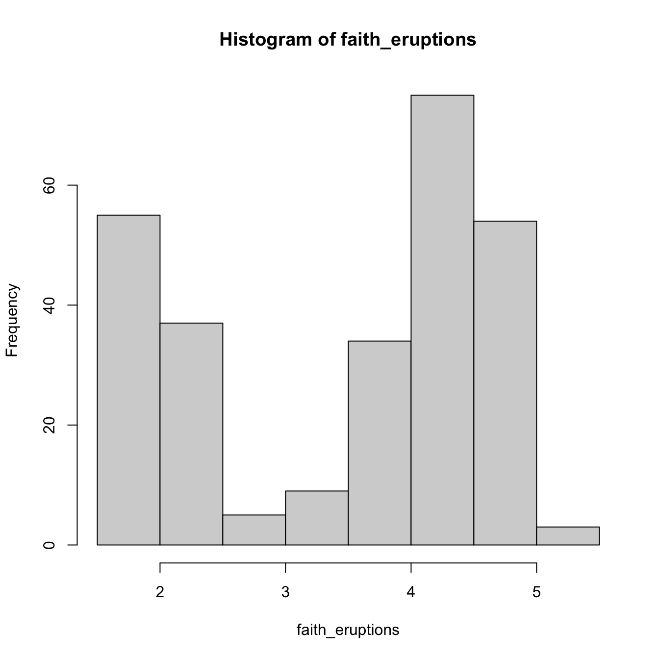


# List that contains several objects
str(histo)
## List of 6
##  $ breaks  : num [1:9] 1.5 2 2.5 3 3.5 4 4.5 5 5.5
##  $ counts  : int [1:8] 55 37 5 9 34 75 54 3
##  $ density : num [1:8] 0.4044 0.2721 0.0368 0.0662 0.25 ...
##  $ mids    : num [1:8] 1.75 2.25 2.75 3.25 3.75 4.25 4.75 5.25
##  $ xname   : chr "faith_eruptions"
##  $ equidist: logi TRUE
##  - attr(*, "class")= chr "histogram"

# With relative frequencies
hist(faith_eruptions, probability = TRUE)


# Choosing the breaks
# t0 = min(faithE), h = 0.25
Bk <- seq(min(faith_eruptions), max(faith_eruptions), by = 0.25)
hist(faith_eruptions, probability = TRUE, breaks = Bk)
rug(faith_eruptions) # Plotting the sample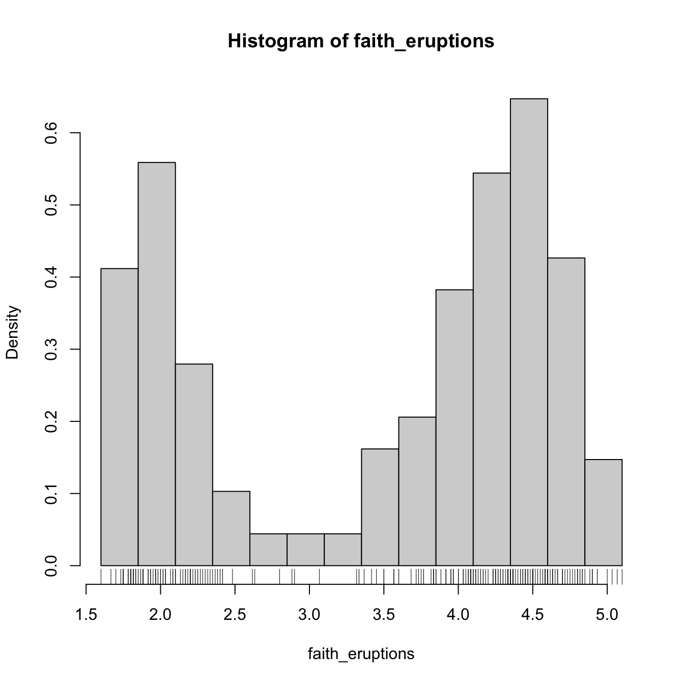

Exercise 2.1 For iris$Sepal.Length, compute:

The histogram of relative frequencies with five bins.
The histogram of absolute frequencies with $t_0=4.3$ and $h=1.$

Add the rug of the data for both histograms.

The analysis of $\hat{f}_\mathrm{H}(x;t_0,h)$ as a random variable is simple, once one recognizes that the bin counts $v_k$ are distributed as $\mathrm{B}(n,p_k),$ with $p_k:=\mathbb{P}[X\in B_k]=\int_{B_k} f(t)\,\mathrm{d}t.$¹⁸ If $f$ is continuous, then by the integral mean value theorem, $p_k=hf(\xi_{k,h})$ for a $\xi_{k,h}\in(t_k,t_{k+1}).$ Assume that $k\in\mathbb{Z}$ is such that $x\in B_k=\lbrack t_k,t_{k+1}).$¹⁹ Therefore:

\[\begin{align} \begin{split} \mathbb{E}[\hat{f}_\mathrm{H}(x;t_0,h)]&=\frac{np_k}{nh}=f(\xi_{k,h}),\\ \mathbb{V}\mathrm{ar}[\hat{f}_\mathrm{H}(x;t_0,h)]&=\frac{np_k(1-p_k)}{n^2h^2}=\frac{f(\xi_{k,h})(1-hf(\xi_{k,h}))}{nh}. \end{split} \tag{2.2} \end{align}\]

The results above yield interesting insights:

If $h\to0,$ then $\xi_{k,h}\to x,$²⁰ resulting in $f(\xi_{k,h})\to f(x),$ and thus (2.1) becomes an asymptotically (when $h\to0$) unbiased estimator of $f(x).$
But if $h\to0,$ the variance increases. For decreasing the variance, $nh\to\infty$ is required.
The variance is directly dependent on $f(\xi_{k,h})(1-hf(\xi_{k,h}))\to f(x)$ (as $h\to0$), hence there is more variability at regions with higher density.

A more detailed analysis of the histogram can be seen in Section 3.2.2 in Scott (2015). We skip it since the detailed asymptotic analysis for the more general kernel density estimator will be given in Section 2.2.

Exercise 2.2 Given (2.2), obtain $\mathrm{MSE}[\hat{f}_\mathrm{H}(x;t_0,h)].$ What should happen in order to have $\mathrm{MSE}[\hat{f}_\mathrm{H}(x;t_0,h)]\to0$?

Clearly, the shape of the histogram depends on:

$t_0,$ since the separation between bins happens at $t_0+kh,$ $k\in\mathbb{Z};$
$h,$ which controls the bin size and the effective number of bins for aggregating the sample.

We focus first on exploring the dependence on $t_0,$ as it serves to motivate the next density estimator.

# Sample from a U(0, 1)
set.seed(1234567)
u <- runif(n = 100)

# Bins for t0 = 0, h = 0.2
Bk1 <- seq(0, 1, by = 0.2)

# Bins for t0 = -0.1, h = 0.2
Bk2 <- seq(-0.1, 1.1, by = 0.2)

# Comparison of histograms for different t0's
hist(u, probability = TRUE, breaks = Bk1, ylim = c(0, 1.5),
     main = "t0 = 0, h = 0.2")
rug(u)
abline(h = 1, col = 2)
hist(u, probability = TRUE, breaks = Bk2, ylim = c(0, 1.5),
     main = "t0 = -0.1, h = 0.2")
rug(u)
abline(h = 1, col = 2)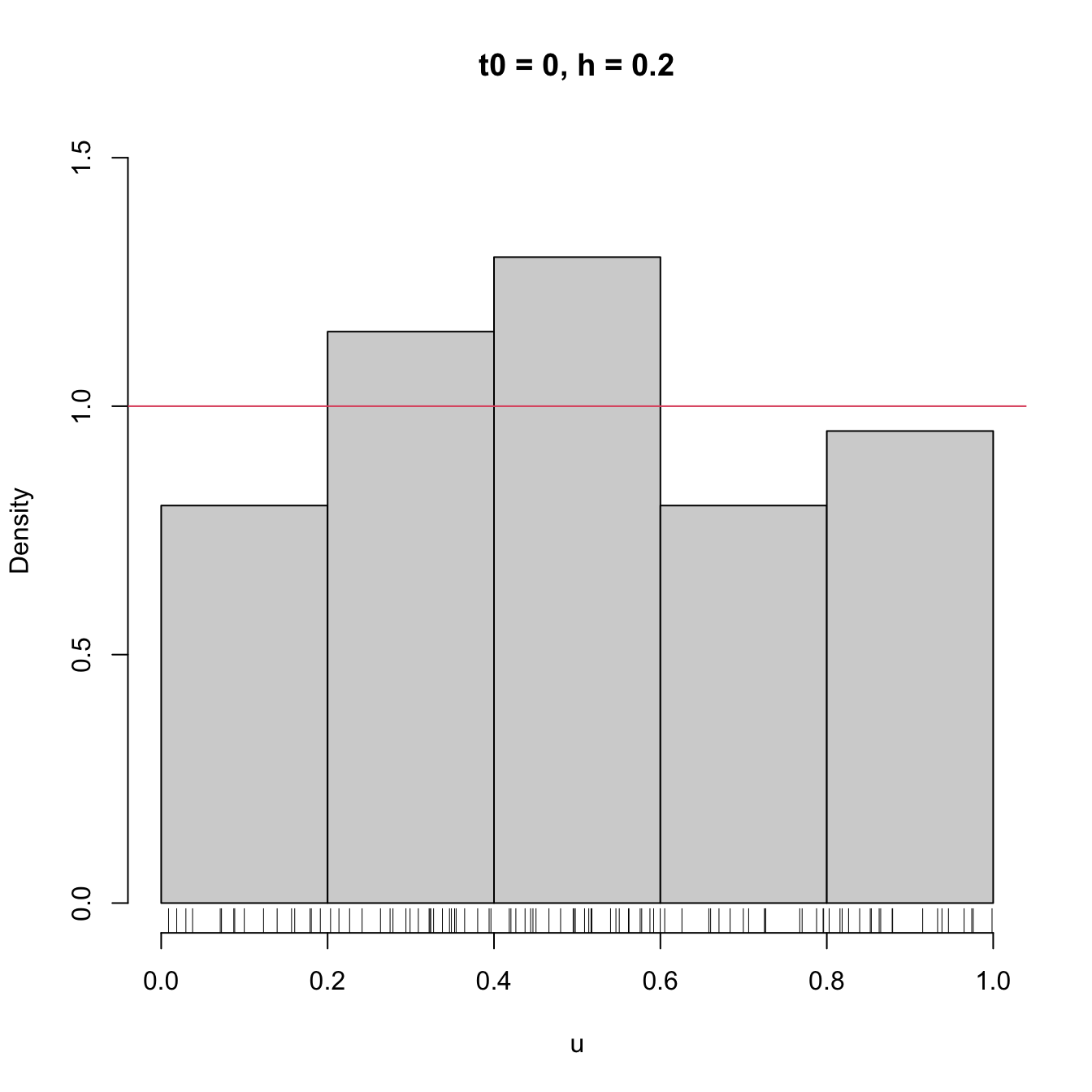

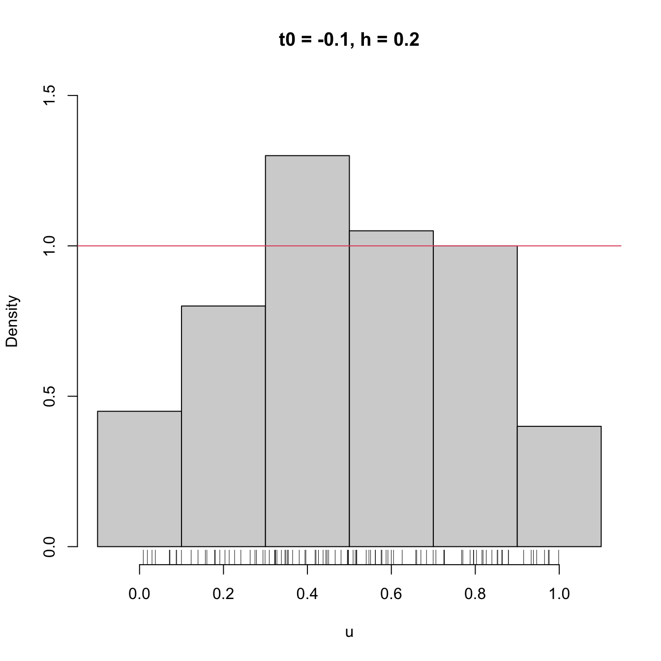
$The dependence of the histogram on the origin $t_0.$ The red curve represents the uniform pdf.$ $The dependence of the histogram on the origin $t_0.$ The red curve represents the uniform pdf.$

Figure 2.2: The dependence of the histogram on the origin $t_0.$ The red curve represents the uniform pdf.

High dependence on $t_0$ also happens when estimating densities that are not compactly supported. The following snippet of code points towards it.

# Sample 50 points from a N(0, 1) and 25 from a N(3.25, 0.5)
set.seed(1234567)
samp <- c(rnorm(n = 50, mean = 0, sd = 1),
          rnorm(n = 25, mean = 3.25, sd = sqrt(0.5)))

# min and max for choosing Bk1 and Bk2
range(samp)
## [1] -2.082486  4.344547

# Comparison
Bk1 <- seq(-2.5, 5, by = 0.5)
Bk2 <- seq(-2.25, 5.25, by = 0.5)
hist(samp, probability = TRUE, breaks = Bk1, ylim = c(0, 0.5),
     main = "t0 = -2.5, h = 0.5")
curve(2/3 * dnorm(x, mean = 0, sd = 1) +
        1/3 * dnorm(x, mean = 3.25, sd = sqrt(0.5)), col = 2, add = TRUE,
      n = 200)
rug(samp)
hist(samp, probability = TRUE, breaks = Bk2, ylim = c(0, 0.5),
     main = "t0 = -2.25, h = 0.5")
curve(2/3 * dnorm(x, mean = 0, sd = 1) +
        1/3 * dnorm(x, mean = 3.25, sd = sqrt(0.5)), col = 2, add = TRUE,
      n = 200)
rug(samp)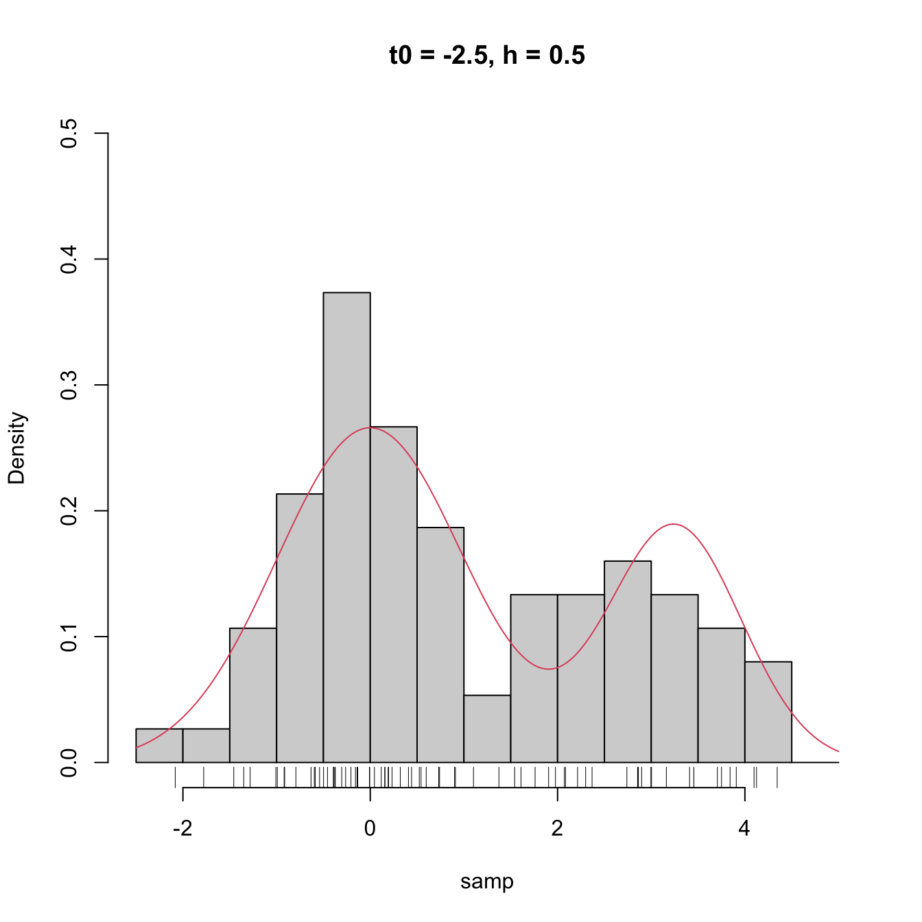

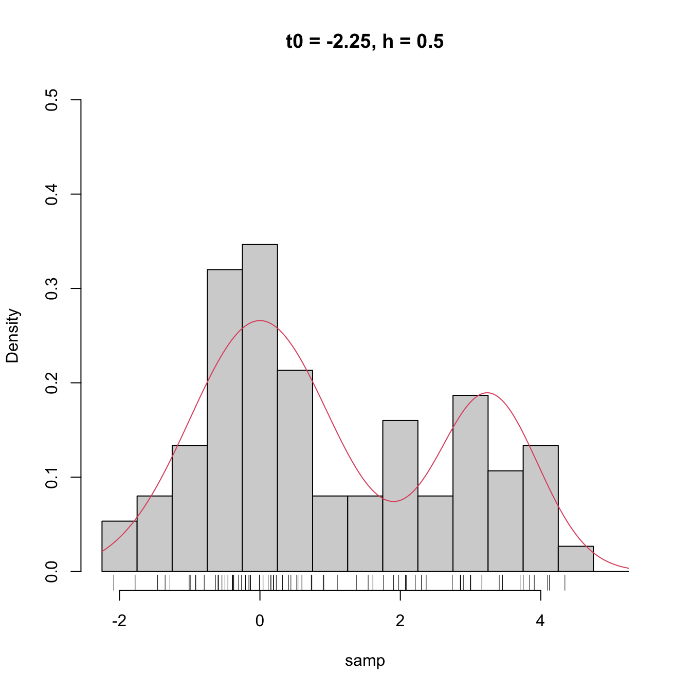
$The dependence of the histogram on the origin $t_0$ for non-compactly supported densities. The red curve represents the underlying pdf, a mixture of two normals.$ $The dependence of the histogram on the origin $t_0$ for non-compactly supported densities. The red curve represents the underlying pdf, a mixture of two normals.$

Figure 2.3: The dependence of the histogram on the origin $t_0$ for non-compactly supported densities. The red curve represents the underlying pdf, a mixture of two normals.

Clearly, the subjectivity introduced by the dependence of $t_0$ is something that we would like to get rid of. We can do so by allowing the bins to be dependent on $x$ (the point at which we want to estimate $f(x)$), rather than fixing them beforehand.

2.1.2 Moving histogram

An alternative to avoid the dependence on $t_0$ is the moving histogram, also known as the naive density estimator.²¹ The idea is to aggregate the sample $X_1,\ldots,X_n$ in intervals of the form $(x-h, x+h)$ and then use its relative frequency in $(x-h,x+h)$ to approximate the density at $x,$ which can be expressed as

\[\begin{align*} f(x)&=F'(x)\\ &=\lim_{h\to0^+}\frac{F(x+h)-F(x-h)}{2h}\\ &=\lim_{h\to0^+}\frac{\mathbb{P}[x-h<X<x+h]}{2h}. \end{align*}\]

Recall the differences with the histogram: the intervals depend on the evaluation point $x$ and are centered about it. This allows us to directly estimate $f(x)$ (without the proxy $f(x_0)$) using an estimate based on the symmetric derivative of $F$ at $x,$ instead of employing an estimate based on the forward derivative of $F$ at $x_0.$

More precisely, given a bandwidth $h>0,$ the naive density estimator builds a piecewise constant function by considering the relative frequency of $X_1,\ldots,X_n$ inside $(x-h,x+h)$:

\[\begin{align} \hat{f}_\mathrm{N}(x;h):=\frac{1}{2nh}\sum_{i=1}^n1_{\{x-h<X_i<x+h\}}. \tag{2.3} \end{align}\]

Figure 2.4 shows the moving histogram for the same sample used in Figure 2.3, clearly revealing the remarkable improvement with respect to the histograms shown when estimating the underlying density.

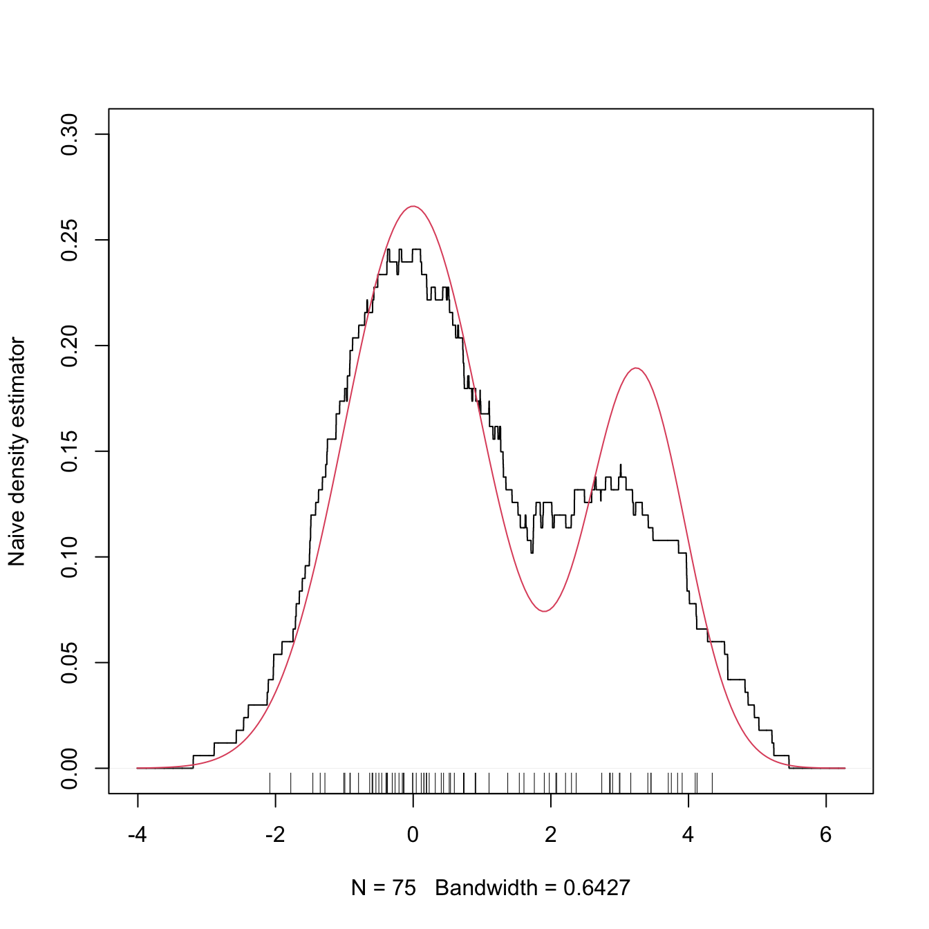
$The naive density estimator $\hat{f}_\mathrm{N}(\cdot;h)$ (black curve). The red curve represents the underlying pdf, a mixture of two normals.$

Figure 2.4: The naive density estimator $\hat{f}_\mathrm{N}(\cdot;h)$ (black curve). The red curve represents the underlying pdf, a mixture of two normals.

Exercise 2.3 Is $\hat{f}_\mathrm{N}(\cdot;h)$ continuous in general? Justify your answer. If the answer is negative, then:

What is the maximum possible number of discontinuities it may have?
What should happen to have fewer discontinuities than its maximum?

Exercise 2.4 Implement your own version of the moving histogram in R. It must be a function that takes as inputs:

a vector with the evaluation points $x;$
sample $X_1,\ldots,X_n;$
bandwidth $h.$

The function must return (2.3) evaluated for each $x.$ Test the implementation by comparing the density of a $\mathcal{N}(0, 1)$ when estimated with $n=100$ observations.

Analogously to the histogram, the analysis of $\hat{f}_\mathrm{N}(x;h)$ as a random variable follows from realizing that

\[\begin{align*} &\sum_{i=1}^n1_{\{x-h<X_i<x+h\}}\sim \mathrm{B}(n,p_{x,h}),\\ &p_{x,h}:=\mathbb{P}[x-h<X<x+h]=F(x+h)-F(x-h). \end{align*}\]

Then:

\[\begin{align} \mathbb{E}[\hat{f}_\mathrm{N}(x;h)]=&\,\frac{F(x+h)-F(x-h)}{2h},\tag{2.4}\\ \mathbb{V}\mathrm{ar}[\hat{f}_\mathrm{N}(x;h)]=&\,\frac{F(x+h)-F(x-h)}{4nh^2}\nonumber\\ &-\frac{(F(x+h)-F(x-h))^2}{4nh^2}.\tag{2.5} \end{align}\]

Exercise 2.5 Derive expressions (2.4) and (2.5) from the binomial relation indicated above.

Results (2.4) and (2.5) provide interesting insights into the effect of $h$:

If $h\to0,$ then:
- $\mathbb{E}[\hat{f}_\mathrm{N}(x;h)]\to f(x)$ and (2.3) is an asymptotically unbiased estimator of $f(x).$
- $\mathbb{V}\mathrm{ar}[\hat{f}_\mathrm{N}(x;h)]\approx \frac{f(x)}{2nh}-\frac{f(x)^2}{n}\to\infty.$
If $h\to\infty,$ then:
- $\mathbb{E}[\hat{f}_\mathrm{N}(x;h)]\to 0.$
- $\mathbb{V}\mathrm{ar}[\hat{f}_\mathrm{N}(x;h)]\to0.$
The variance shrinks to zero if $nh\to\infty.$²² So both the bias and the variance can be reduced if $n\to\infty,$ $h\to0,$ and $nh\to\infty,$ simultaneously.
The variance is almost proportional²³ to $f(x).$

The animation in Figure 2.5 illustrates the previous points and gives insights into how the performance of (2.3) varies smoothly with $h.$

Figure 2.5: Bias and variance for the moving histogram. The animation shows how for small bandwidths the bias of $\hat{f}_\mathrm{N}(x;h)$ on estimating $f(x)$ is small, but the variance is high, and how for large bandwidths the bias is large and the variance is small. The variance is visualized through the asymptotic $95\%$ confidence intervals for $\hat{f}_\mathrm{N}(x;h).$ Application available here.

The estimator (2.3) raises an important question:

Why give the same weight to all $X_1,\ldots,X_n$ in $(x-h, x+h)$ for approximating $\frac{\mathbb{P}[x-h<X<x+h]}{2h}$?

We are estimating $f(x)=F'(x)$ by estimating $\frac{F(x+h)-F(x-h)}{2h}$ through the relative frequency of $X_1,\ldots,X_n$ in the interval $(x-h,x+h).$ Therefore, it seems reasonable that the data points closer to $x$ are more important to assess the infinitesimal probability of $x$ than the ones further away. This observation shows that (2.3) is indeed a particular case of a wider and more sensible class of density estimators, which we will see next.

2.2 Kernel density estimation

The moving histogram (2.3) can be equivalently written as

\[\begin{align} \hat{f}_\mathrm{N}(x;h)&=\frac{1}{2nh}\sum_{i=1}^n1_{\{x-h<X_i<x+h\}}\nonumber\\ &=\frac{1}{nh}\sum_{i=1}^n\frac{1}{2}1_{\left\{-1<\frac{x-X_i}{h}<1\right\}}\nonumber\\ &=\frac{1}{nh}\sum_{i=1}^nK\left(\frac{x-X_i}{h}\right), \tag{2.6} \end{align}\]

with $K(z)=\frac{1}{2}1_{\{-1<z<1\}}.$ Interestingly, $K$ is a uniform density in $(-1,1)$! This means that, when approximating

\[\begin{align*} \mathbb{P}[x-h<X<x+h]=\mathbb{P}\left[-1<\frac{x-X}{h}<1\right] \end{align*}\]

by (2.6), we are giving equal weight to all the points $X_1,\ldots,X_n.$ The generalization of (2.6) to non-uniform weighting is now obvious: replace $K$ with an arbitrary density! Then $K$ is known as a kernel. As it is commonly²⁴ assumed, we consider $K$ to be a density that is symmetric and unimodal at zero. This generalization provides the definition of the kernel density estimator (kde):²⁵

\[\begin{align} \hat{f}(x;h):=\frac{1}{nh}\sum_{i=1}^nK\left(\frac{x-X_i}{h}\right). \tag{2.7} \end{align}\]

A common notation is $K_h(z):=\frac{1}{h}K\left(\frac{z}{h}\right),$ the so-called scaled kernel, so that the kde is written as $\hat{f}(x;h)=\frac{1}{n}\sum_{i=1}^nK_h(x-X_i).$

Figure 2.6: Construction of the kernel density estimator. The animation shows how bandwidth and kernel affect the density estimate, and how the kernels are rescaled densities with modes at the data points. Application available here.

It is useful to recall (2.7) with the normal kernel. If that is the case, then $K_h(x-X_i)=\phi_h(x-X_i)$ and the kernel is the density of a $\mathcal{N}(X_i,h^2).$ Thus the bandwidth $h$ can be thought of as the standard deviation of a normal density with mean $X_i,$ and the kde (2.7) as a data-driven mixture of those densities. Figure 2.6 illustrates the construction of the kde and the bandwidth and kernel effects.

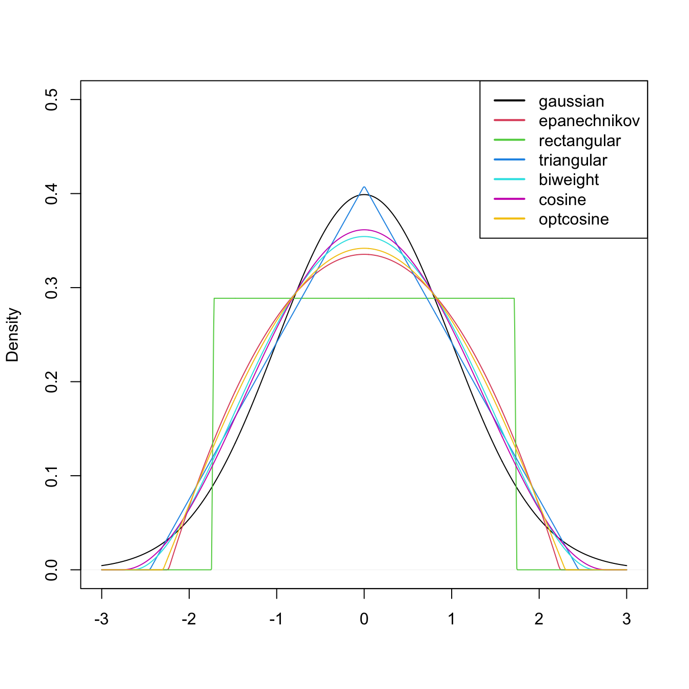
Figure 2.7: Several scaled kernels from R’s density function. See (2.9) in the remark below for the different parametrization.

Several types of kernels are possible. Figure 2.7 illustrates the form of several implemented in R’s density function. The most popular is the normal kernel $K(z)=\phi(z),$ although the Epanechnikov kernel, $K(z)=\frac{3}{4}(1-z^2)1_{\{|z|<1\}},$ is the most efficient.²⁶ The rectangular kernel $K(z)=\frac{1}{2}1_{\{|z|<1\}}$ yields the moving histogram as a particular case. Importantly, the kde inherits the smoothness properties of the kernel. That means, for example, that (2.7) with a normal kernel is infinitely differentiable. But with an Epanechnikov kernel, (2.7) is not differentiable, and with a rectangular kernel is not even continuous. However, if a certain smoothness is guaranteed (continuity at least), the choice of the kernel has little importance in practice, at least in comparison with the much more critical choice of the bandwidth $h.$

The computation of the kde in R is done through the density function. The function automatically chooses the bandwidth $h$ using a data-driven criterion²⁷ referred to as a bandwidth selector. Bandwidth selectors will be studied in detail in Section 2.4.

# Sample 100 points from a N(0, 1)
set.seed(1234567)
samp <- rnorm(n = 100, mean = 0, sd = 1)

# Quickly compute a kde and plot the density object
# Automatically chooses bandwidth and uses normal kernel
plot(density(x = samp))

# Select a particular bandwidth (0.5) and kernel (Epanechnikov)
lines(density(x = samp, bw = 0.5, kernel = "epanechnikov"), col = 2)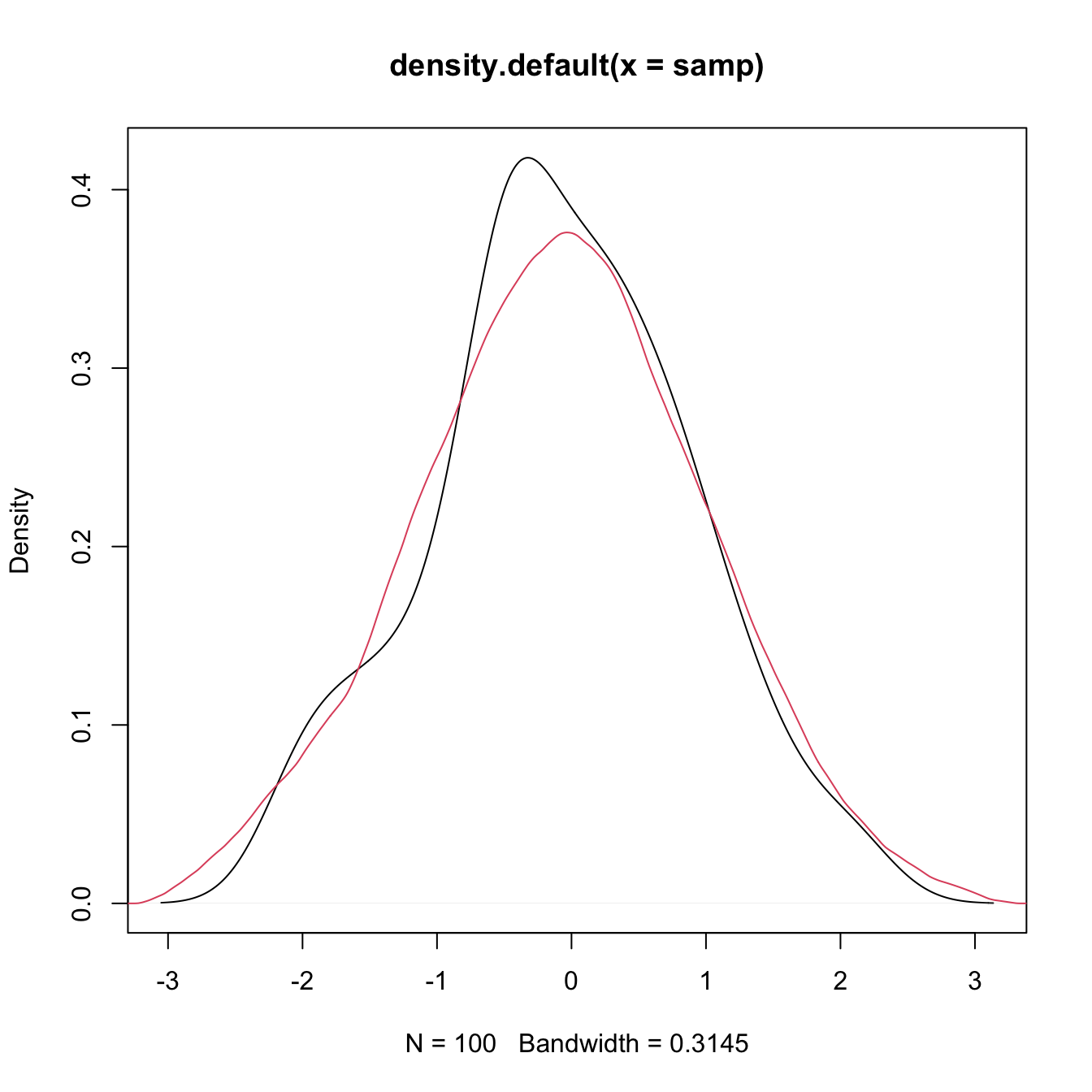


# density() automatically chooses the interval for plotting the kde
# (observe that the black line goes to roughly between -3 and 3)
# This can be tuned using "from" and "to"
plot(density(x = samp, from = -4, to = 4), xlim = c(-5, 5))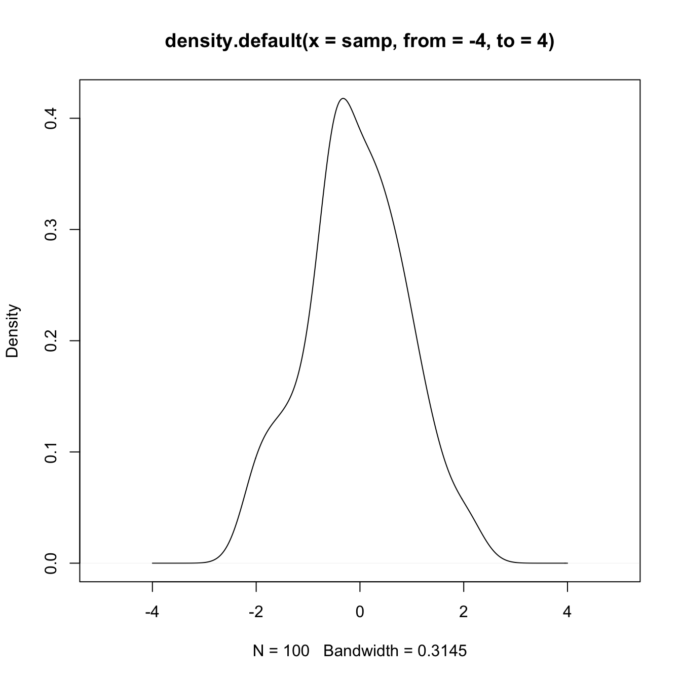


# The density object is a list
kde <- density(x = samp, from = -5, to = 5, n = 1024)
str(kde)
## List of 7
##  $ x        : num [1:1024] -5 -4.99 -4.98 -4.97 -4.96 ...
##  $ y        : num [1:1024] 4.91e-17 2.97e-17 1.86e-17 2.53e-17 3.43e-17 ...
##  $ bw       : num 0.315
##  $ n        : int 100
##  $ call     : language density.default(x = samp, n = 1024, from = -5, to = 5)
##  $ data.name: chr "samp"
##  $ has.na   : logi FALSE
##  - attr(*, "class")= chr "density"
# Note that the evaluation grid "x" is not directly controlled, only through
# "from, "to", and "n" (better use powers of 2)
plot(kde$x, kde$y, type = "l")
curve(dnorm(x), col = 2, add = TRUE) # True density
rug(samp)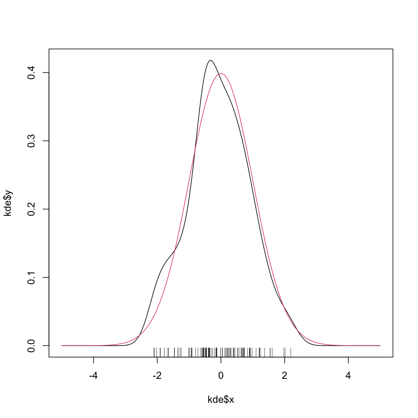

Exercise 2.6 Employing the normal kernel:

Estimate and plot the density of faithful$eruptions.
Create a new plot and superimpose different density estimations with bandwidths equal to $0.1,$ $0.5,$ and $1.$
Get the density estimate at exactly the point $x=3.1$ using $h=0.15.$

We next introduce an important remark about the use of the density function. Before that, we need some notation. From now on, we consider the integrals to be over $\mathbb{R}$ if not stated otherwise. In addition, we denote

\[\begin{align*} \mu_2(K):=\int z^2 K(z)\,\mathrm{d}z \end{align*}\]

to the second-order moment²⁸ of $K.$

Remark. The kernel, say $\tilde K,$ employed in density uses a parametrization that guarantees that $\mu_2(\tilde K)=1.$ This implies that the variance of the scaled kernel is $h^2,$ that is, that $\mu_2(\tilde K_h)=h^2.$ These normalized kernels may be different from the ones we have considered in the exposition. For example, the uniform kernel $K(z)=\frac{1}{2}1_{\{-1<z<1\}},$ for which $\mu_2(K)=\frac{1}{3},$ is implemented in R as $\tilde K(z)=\frac{1}{2\sqrt{3}}1_{\{-\sqrt{3}<z<\sqrt{3}\}}$ (observe in Figure 2.7 that the rectangular kernel takes the value $\frac{1}{2\sqrt{3}}\approx 0.29$).

The density’s normalized kernel $\tilde K$ can be obtained from $K,$ and vice versa, with a straightforward derivation. On the one hand, since $\mu_2(K) = \int z^2 K(z),$

\[\begin{align} 1 &= \int \frac{z^2}{\mu_2(K)} K(z)\,\mathrm{d}z\nonumber\\ &= \int t^2 K\big(\mu_2(K)^{1/2} t\big)\mu_2(K)^{1/2}\,\mathrm{d}t\tag{2.8} \end{align}\]

by making the change of variables $t=\frac{z}{\mu_2(K)^{1/2}}$ in the second equality. Now, based on (2.8), define

\[\begin{align} \tilde K(z) := \mu_2(K)^{1/2}K\big(\mu_2(K)^{1/2} z\big) \tag{2.9} \end{align}\]

and this is a kernel that satisfies $\mu_2(\tilde K)=\int t^2 \tilde K(t)\,\mathrm{d}t = 1$ and is a density unimodal about $0.$ It is indeed the kernel employed by density.

Therefore, if we consider a bandwidth $h$ for the normalized kernel $\tilde K$ (resulting $\tilde K_h$), we have that

\[\begin{align*} \tilde K_h(z) = \frac{\mu_2(K)^{1/2}}{h} K\left(\frac{\mu_2(K)^{1/2}z}{h}\right) = K_{\tilde h}(z) \end{align*}\]

where

\[\begin{align*} \tilde h := \mu_2(K)^{-1/2}h. \end{align*}\]

As a consequence, a normalized kernel $\tilde K$ with a given bandwidth $h$ (for example, the one considered in density’s bw) has an associated scaled bandwidth $\tilde h$ for the unnormalized kernel $K.$

The following code numerically illustrates the difference between $\tilde K$ and $K$ for the Epanechnikov kernel.

# Implementation of the Epanechnikov based on the theory
K_Epa <- function(z, h = 1) 3 / (4 * h) * (1 - (z / h)^2) * (abs(z) < h)
mu2_K_Epa <- integrate(function(z) z^2 * K_Epa(z), lower = -1, upper = 1)$value

# Epanechnikov kernel by R
h <- 0.5
plot(density(0, kernel = "epanechnikov", bw = h))

# Build the equivalent bandwidth
h_tilde <- h / sqrt(mu2_K_Epa)
curve(K_Epa(x, h = h_tilde), add = TRUE, col = 2)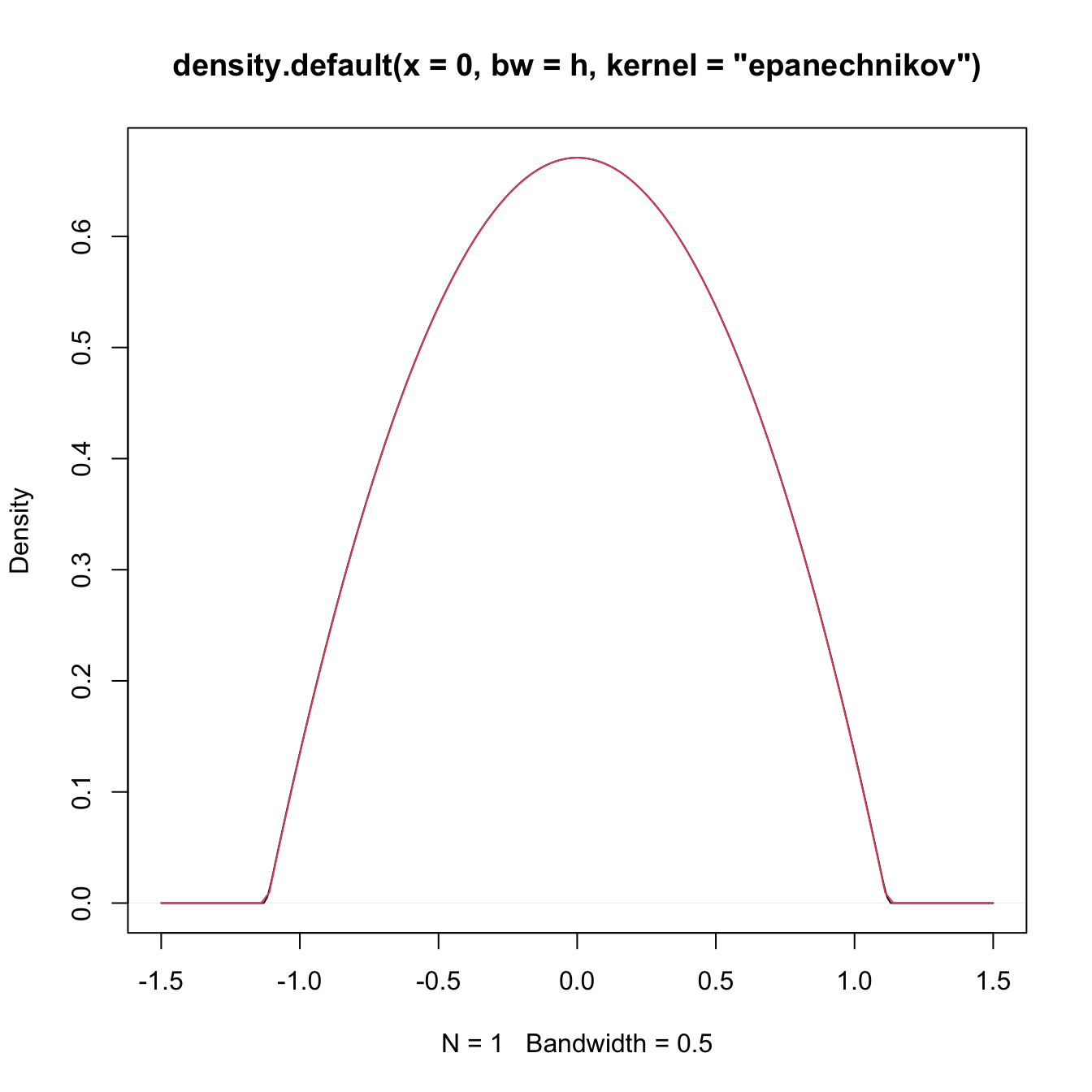


# The other way around
h_tilde <- 2
h <- h_tilde * sqrt(mu2_K_Epa)
curve(K_Epa(x, h = h_tilde), from = -3, to = 3, col = 2)
lines(density(0, kernel = "epanechnikov", bw = h))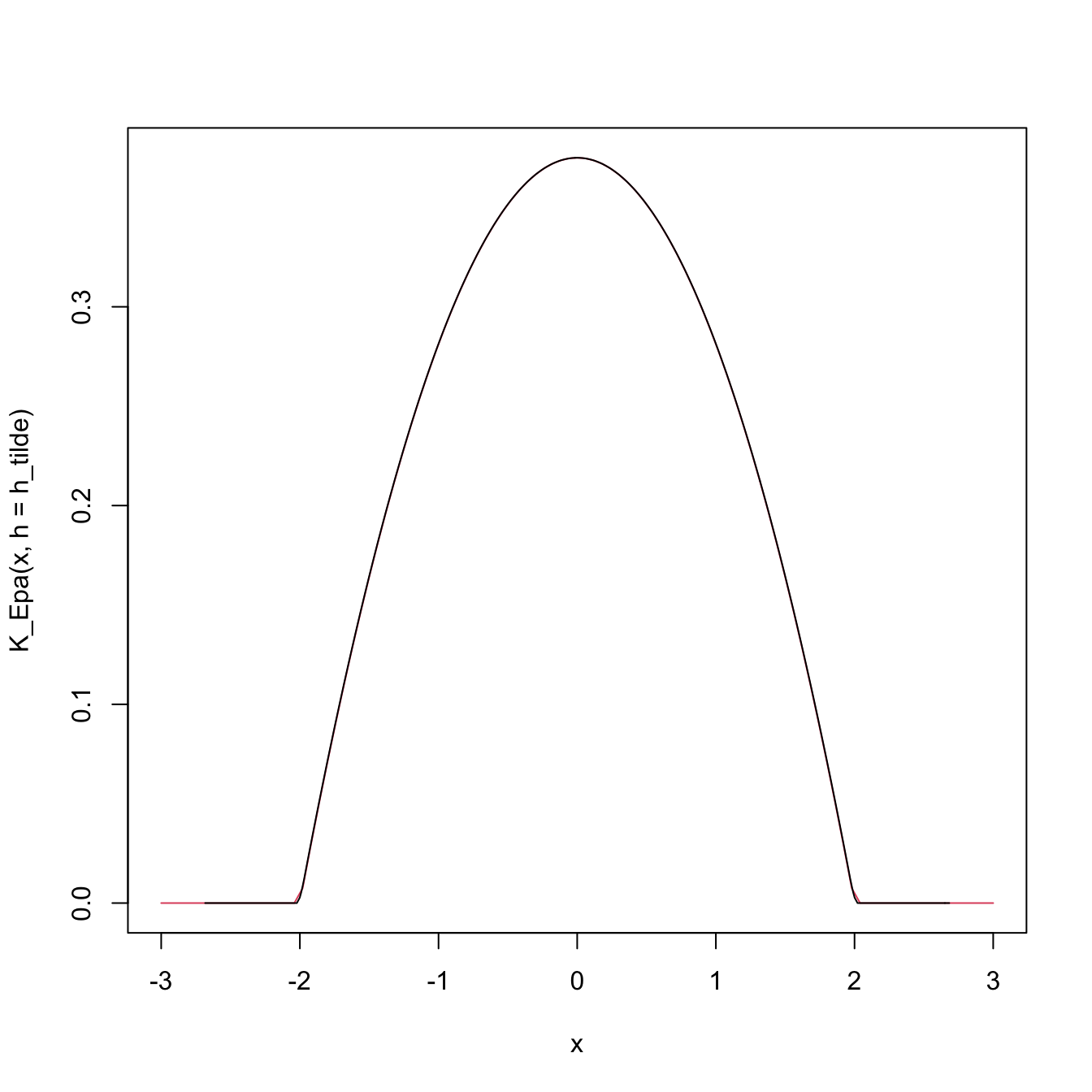

Exercise 2.7 Obtain the kernel $\tilde K$ for:

the normal kernel $K(z)=\phi(z);$
the Epanechnikov kernel $K(z)=\frac{3}{4}(1-z^2)1_{\{|z|<1\}};$
the kernel $K(z)=(1-|z|)1_{\{|z|<1\}}.$

Exercise 2.8 Given $h,$ obtain $\tilde h$ such that $\tilde K_h = K_{\tilde h}$ for:

the uniform kernel $K(z)=\frac{1}{2}1_{\{|z|<1\}};$
the kernel $K(z)=\frac{1}{2\pi}(1+\cos(z))1_{\{|z|<\pi\}};$
the kernel $K(z)=(1-|z|)1_{\{|z|<1\}}.$

Exercise 2.9 Repeat Exercise 2.6, but now considering the Epanechnikov kernel in its unnormalized form. To do so, find the adequate bandwidths to input in density’s bw.

2.3 Asymptotic properties

Asymptotic results serve the purpose of establishing the large-sample ($n\to\infty$) properties of an estimator. One might question why they are useful, since in practice we only have finite sample sizes. Apart from purely theoretical reasons, asymptotic results usually give highly valuable insights into the properties of the estimator, typically much simpler to grasp than those obtained from finite-sample results.²⁹

Throughout this section we will make the following assumptions:

A1.³⁰ The density $f$ is square integrable, twice continuously differentiable, and the second derivative is square integrable.
A2.³¹ The kernel $K$ is a symmetric and bounded pdf with finite second moment and square integrable.
A3.³² $h=h_n$ is a deterministic sequence of positive scalars³³ such that, when $n\to\infty,$ $h\to0$ and $nh\to\infty.$

We need to introduce some notation. The squared integral of a function $f$ is denoted by $R(f):=\int f(x)^2\,\mathrm{d}x.$ The convolution between two real functions $f$ and $g,$ $f*g,$ is the function

\[\begin{align} (f*g)(x):=\int f(x-y)g(y)\,\mathrm{d}y=(g*f)(x).\tag{2.10} \end{align}\]

We are now ready to obtain the bias and variance of $\hat{f}(x;h).$ Recall that is not possible to apply the “binomial trick” we used previously for the histogram and moving histogram: now the estimator is not piecewise constant. Instead, we use the linearity of the kde and the convolution definition. For the expectation, we have

\[\begin{align} \mathbb{E}[\hat{f}(x;h)]&=\frac{1}{n}\sum_{i=1}^n\mathbb{E}[K_h(x-X_i)]\nonumber\\ &=\int K_h(x-y)f(y)\,\mathrm{d}y\nonumber\\ &=(K_h * f)(x).\tag{2.11} \end{align}\]

Similarly, the variance is obtained as

\[\begin{align} \mathbb{V}\mathrm{ar}[\hat{f}(x;h)]&=\frac{1}{n}((K_h^2*f)(x)-(K_h*f)^2(x)).\tag{2.12} \end{align}\]

These two expressions are exact, but hard to interpret. Equation (2.11) indicates that the estimator is biased,³⁴ but it does not explicitly differentiate the effects of kernel, bandwidth, and density on the bias. The same happens with (2.12), yet more emphasized. Clarity is why the following asymptotic expressions are preferred.

Theorem 2.1 Under A1–A3, the bias and variance of the kde at $x$ are

\[\begin{align} \mathrm{Bias}[\hat{f}(x;h)]&=\frac{1}{2}\mu_2(K)f''(x)h^2+o(h^2),\tag{2.13}\\ \mathbb{V}\mathrm{ar}[\hat{f}(x;h)]&=\frac{R(K)}{nh}f(x)+o((nh)^{-1}).\tag{2.14} \end{align}\]

Proof. For the bias we consider the change of variables $z=\frac{x-y}{h},$ $y=x-hz,$ $\mathrm{d}y=-h\,\mathrm{d}z.$ The integral limits flip and we have

\[\begin{align} \mathbb{E}[\hat{f}(x;h)]&=\int K_h(x-y)f(y)\,\mathrm{d}y\nonumber\\ &=\int K(z)f(x-hz)\,\mathrm{d}z.\tag{2.15} \end{align}\]

Since $h\to0,$ an application of a second-order Taylor expansion gives

\[\begin{align} f(x-hz)=&\,f(x)-f'(x)hz+\frac{f''(x)}{2}h^2z^2\nonumber\\ &+o(h^2z^2). \tag{2.16} \end{align}\]

Substituting (2.16) in (2.15), and bearing in mind that $K$ is a symmetric density about $0,$ we have

\[\begin{align*} \int K(z)&f(x-hz)\,\mathrm{d}z\\ =&\,\int K(z)\Big\{f(x)-f'(x)hz+\frac{f''(x)}{2}h^2z^2\\ &+o(h^2z^2)\Big\}\,\mathrm{d}z\\ =&\,f(x)+\frac{1}{2}\mu_2(K)f''(x)h^2+o(h^2), \end{align*}\]

which provides (2.13).

For the variance, first note that

\[\begin{align} \mathbb{V}\mathrm{ar}[\hat{f}(x;h)]&=\frac{1}{n^2}\sum_{i=1}^n\mathbb{V}\mathrm{ar}[K_h(x-X_i)]\nonumber\\ &=\frac{1}{n}\left\{\mathbb{E}[K_h^2(x-X)]-\mathbb{E}[K_h(x-X)]^2\right\}. \tag{2.17} \end{align}\]

The second term of (2.17) is already computed, so we focus on the first. Using the previous change of variables and a first-order Taylor expansion, we have

\[\begin{align} \mathbb{E}[K_h^2(x-X)]&=\frac{1}{h}\int K^2(z)f(x-hz)\,\mathrm{d}z\nonumber\\ &=\frac{1}{h}\int K^2(z)\left\{f(x)+O(hz)\right\}\,\mathrm{d}z\nonumber\\ &=\frac{R(K)}{h}f(x)+O(1). \tag{2.18} \end{align}\]

Plugging (2.17) into (2.18) gives

\[\begin{align*} \mathbb{V}\mathrm{ar}[\hat{f}(x;h)]&=\frac{1}{n}\left\{\frac{R(K)}{h}f(x)+O(1)-O(1)\right\}\\ &=\frac{R(K)}{nh}f(x)+O(n^{-1})\\ &=\frac{R(K)}{nh}f(x)+o((nh)^{-1}), \end{align*}\]

since $n^{-1}=o((nh)^{-1}).$

Remark. Integrating little-$o$’s is a tricky issue. In general, integrating a $o^x(1)$ quantity, possibly dependent on $x$ (this is emphasized with the superscript), does not provide an $o(1).$ In other words: $\int o^x(1)\,\mathrm{d}x\neq o(1).$ If the previous inequality becomes an equality, then the limits and integral will be interchangeable. But this is not always true – only if certain conditions are met, recall the DCT (Theorem 1.12). If one wants to be completely rigorous on the two implicit commutations of integrals and limits that took place in the proof, it is necessary to have explicit control of the remainder via Taylor’s theorem (Theorem 1.11) and then apply the DCT. This has been skipped for simplicity in the exposition.

The bias and variance expressions (2.13) and (2.14) yield interesting insights (see Figure 2.5 for visualizations thereof):

The bias decreases with $h$ quadratically. In addition, the bias at $x$ is directly proportional to $f''(x).$ This has an interesting interpretation:
- The bias is negative where $f$ is concave, i.e., $\{x\in\mathbb{R}:f''(x)<0\}.$ These regions correspond to peaks and modes of $f,$ where the kde underestimates $f$ (it tends to be below $f$).
- Conversely, the bias is positive where $f$ is convex, i.e., $\{x\in\mathbb{R}:f''(x)>0\}.$ These regions correspond to valleys and tails of $f,$ where the kde overestimates $f$ (it tends to be above $f$).
- The “wilder” the curvature $f'',$ the harder to estimate $f.$ Flat density regions are easier to estimate than wiggling regions with high curvature (e.g., with several modes).
The variance depends directly on $f(x).$ The higher the density, the more variable the kde is. Interestingly, the variance decreases as a factor of $(nh)^{-1},$ a consequence of $nh$ playing the role of the effective sample size for estimating $f(x).$ The effective sample size can be thought of as the amount of data³⁵ in the neighborhood of $x$ that is employed for estimating $f(x).$

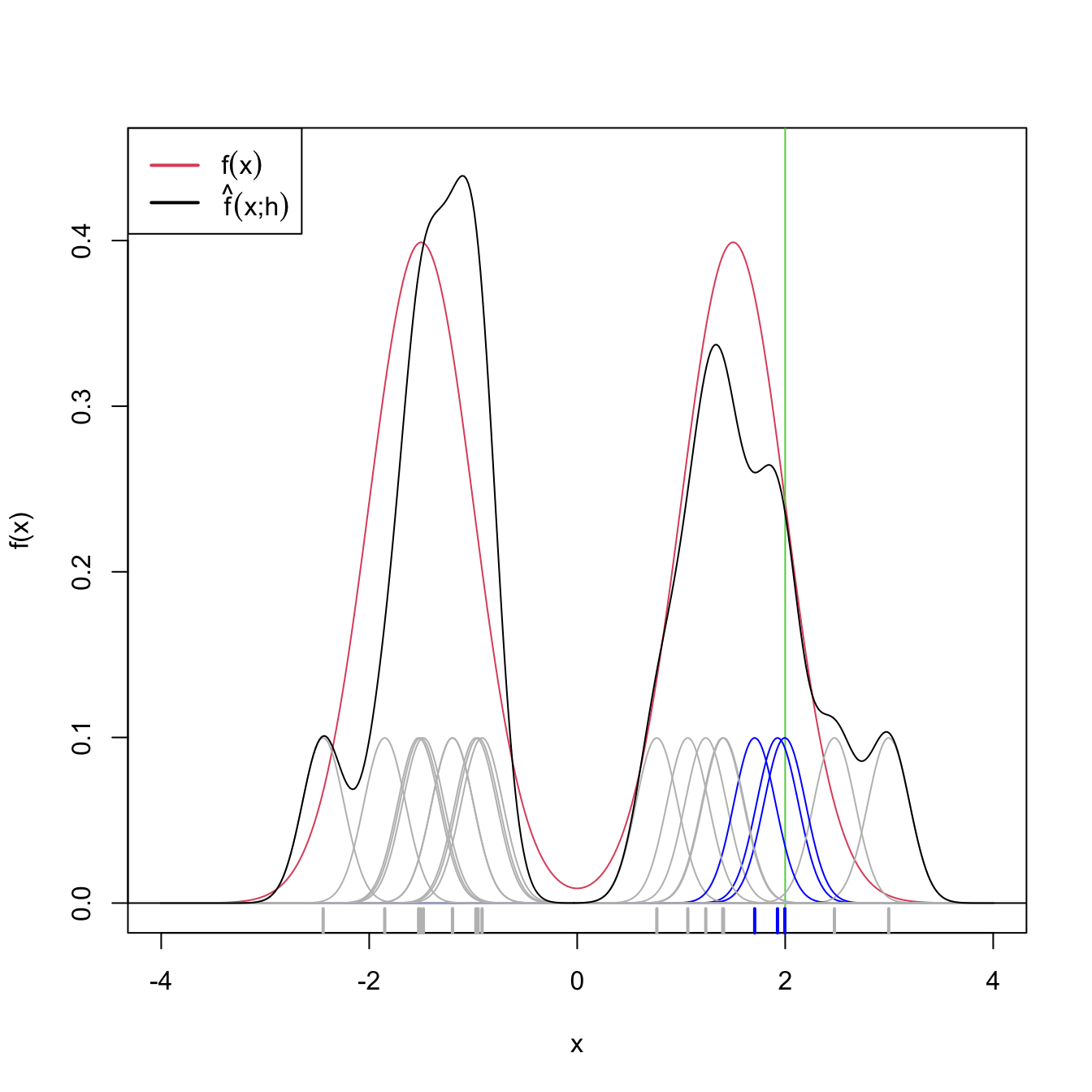
$Illustration of the effective sample size for estimating $f(x)$ at $x=2.$ In blue, the kernels with contribution to the kde larger than $0.01.$ In gray, rest of the kernels. Only $3$ observations are effectively employed for estimating $f(2)$ by $\hat f(2;0.2),$ despite the sample size being $n=20$.$

Figure 2.8: Illustration of the effective sample size for estimating $f(x)$ at $x=2.$ In blue, the kernels with contribution to the kde larger than $0.01.$ In gray, rest of the kernels. Only $3$ observations are effectively employed for estimating $f(2)$ by $\hat f(2;0.2),$ despite the sample size being $n=20$.

Exercise 2.10 Using Example 1.5 and Theorem 2.1, show that:

$\hat{f}(x;h)=f(x)+O(h^2)+O_\mathbb{P}\big((nh)^{-1/2}\big).$
$\hat{f}(x;h)=f(x)(1+o_\mathbb{P}(1)).$

The MSE of the kde is trivial to obtain from the bias and variance.

Corollary 2.1 Under A1–A3, the MSE of the kde at $x$ is

\[\begin{align} \mathrm{MSE}[\hat{f}(x;h)]=\,&\frac{\mu^2_2(K)}{4}(f''(x))^2h^4+\frac{R(K)}{nh}f(x)\nonumber\\ &+o(h^4+(nh)^{-1}).\tag{2.19} \end{align}\]

Therefore, the kde is pointwise consistent in MSE, i.e., $\hat{f}(x;h)\stackrel{2}{\longrightarrow}f(x).$

Exercise 2.11 Prove Corollary 2.1 using Theorem 2.1 and Proposition 1.7.

Note that, due to the MSE-consistency of $\hat{f}(x;h),$ \[\begin{align*} \hat{f}(x;h)\stackrel{2}{\longrightarrow}f(x)\implies\hat{f}(x;h)\stackrel{\mathbb{P}}{\longrightarrow}f(x)\implies\hat{f}(x;h)\stackrel{d}{\longrightarrow}f(x) \end{align*}\] under A1–A2. However, these results are not useful for quantifying the randomness of $\hat{f}(x;h)$: the convergence is towards the degenerate random variable $f(x),$ for a given $x\in\mathbb{R}.$³⁶ For that reason, we now turn our attention to the asymptotic normality of the estimator.

Theorem 2.2 Assume that $\int K^{2+\delta}(z)\,\mathrm{d}z<\infty\,$³⁷ for some $\delta>0.$ Then, under A1–A3,

\[\begin{align} &\sqrt{nh}\left(\hat{f}(x;h)-\mathbb{E}[\hat{f}(x;h)]\right)\stackrel{d}{\longrightarrow}\mathcal{N}(0,R(K)f(x)).\tag{2.20} \end{align}\]

Additionally, if $nh^5=O(1),$ then

\[\begin{align} &\sqrt{nh}\left(\hat{f}(x;h)-f(x)-\frac{1}{2}\mu_2(K)f''(x)h^2\right)\stackrel{d}{\longrightarrow}\mathcal{N}(0,R(K)f(x)).\tag{2.21} \end{align}\]

Proof. First note that $K_h(x-X_n)$ is a sequence of independent but not identically distributed random variables: $h=h_n$ depends on $n.$ Therefore, we look forward to applying Theorem 1.3.

We first prove (2.20). For simplicity, denote $K_i:=K_h(x-X_i),$ $i=1,\ldots,n.$ From the proof of Theorem 2.1 we know that $\mathbb{E}[K_i]=\mathbb{E}[\hat{f}(x;h)]=f(x)+o(1)$ and

\[\begin{align*} s_n^2&=\sum_{i=1}^n \mathbb{V}\mathrm{ar}[K_i]\\ &=n^2\mathbb{V}\mathrm{ar}[\hat{f}(x;h)]\\ &=n\frac{R(K)}{h}f(x)(1+o(1)). \end{align*}\]

An application of the $C_p$ inequality of Lemma 1.1 (first) and Jensen’s inequality (second), gives

\[\begin{align*} \mathbb{E}\left[|K_i-\mathbb{E}[K_i]|^{2+\delta}\right]&\leq C_{2+\delta}\left(\mathbb{E}\left[|K_i|^{2+\delta}\right]+|\mathbb{E}[K_i]|^{2+\delta}\right)\\ &\leq 2C_{2+\delta}\mathbb{E}\left[|K_i|^{2+\delta}\right]\\ &=O\left(\mathbb{E}\left[|K_i|^{2+\delta}\right]\right). \end{align*}\]

In addition, due to a Taylor expansion after $z=\frac{x-y}{h}$ and using that $\int K^{2+\delta}(z)\,\mathrm{d}z<\infty,$

\[\begin{align*} \mathbb{E}\left[|K_i|^{2+\delta}\right]&=\frac{1}{h^{2+\delta}}\int K^{2+\delta}\left(\frac{x-y}{h}\right)f(y)\,\mathrm{d}y\\ &=\frac{1}{h^{1+\delta}}\int K^{2+\delta}(z)f(x-hz)\,\mathrm{d}z\\ &=\frac{1}{h^{1+\delta}}\int K^{2+\delta}(z)(f(x)+o(1))\,\mathrm{d}z\\ &=O\left(h^{-(1+\delta)}\right). \end{align*}\]

Then,

\[\begin{align*} \frac{1}{s_n^{2+\delta}}&\sum_{i=1}^n\mathbb{E}\left[|K_i-\mathbb{E}[K_i]|^{2+\delta}\right]\\ &=\left(\frac{h}{nR(K)f(x)}\right)^{1+\frac{\delta}{2}}(1+o(1))O\left(nh^{-(1+\delta)}\right)\\ &=O\left((nh)^{-\frac{\delta}{2}}\right) \end{align*}\]

and the Lyapunov’s condition is satisfied. As a consequence, by Lyapunov’s CLT and Slutsky’s theorem,

\[\begin{align*} \sqrt{\frac{nh}{R(K)f(x)}}&(\hat{f}(x;h)-\mathbb{E}[\hat{f}(x;h)])\\ &=(1+o(1))\frac{1}{s_n}\sum_{i=1}^n(K_i-\mathbb{E}[K_i])\\ &\stackrel{d}{\longrightarrow}\mathcal{N}(0,1) \end{align*}\]

and (2.20) is proved.

To prove (2.21), we consider

\[\begin{align*} \sqrt{nh}&\left(\hat{f}(x;h)-f(x)-\frac{1}{2}\mu_2(K)f''(x)h^2\right)\\ &=\sqrt{nh}(\hat{f}(x;h)-\mathbb{E}[\hat{f}(x;h)]+o(h^2)). \end{align*}\]

Therefore, Slutsky’s theorem and the assumption $nh^5=O(1)$ give

\[\begin{align*} \sqrt{nh}&(\hat{f}(x;h)-\mathbb{E}[\hat{f}(x;h)]+o(h^2))\\ &=\sqrt{nh}\left(\hat{f}(x;h)-\mathbb{E}[\hat{f}(x;h)]+o(\sqrt{nh^5})\right)\\ &=\sqrt{nh}\left(\hat{f}(x;h)-\mathbb{E}[\hat{f}(x;h)]\right)+o(1)\\ &\stackrel{d}{\longrightarrow}\mathcal{N}(0,R(K)f(x)). \end{align*}\]

Remark. Note the rate $\sqrt{nh}$ in the asymptotic normality results. This is different from the standard CLT rate $\sqrt{n}$ (see Theorem 1.2). Indeed, $\sqrt{nh}$ is slower than $\sqrt{n}$: the variance of the limiting normal distribution decreases as $O((nh)^{-1})$ and not as $O(n^{-1}).$ The phenomenon is related to the effective sample size previously illustrated with Figure 2.8.

Exercise 2.12 Using (2.21) and Example 1.6, show that $\hat{f}(x;h)=f(x)+o_\mathbb{P}(1).$

2.4 Bandwidth selection

As we saw in the previous sections, the kde critically depends on the bandwidth employed. The purpose of this section is to introduce objective and automatic bandwidth selectors that attempt to minimize the estimation error of the target density $f.$

The first step is to define a global, rather than local, error criterion. The Integrated Squared Error (ISE),

\[\begin{align*} \mathrm{ISE}[\hat{f}(\cdot;h)]:=\int (\hat{f}(x;h)-f(x))^2\,\mathrm{d}x, \end{align*}\]

is the squared distance between the kde and the target density. The ISE is a random quantity, since it depends directly on the sample $X_1,\ldots,X_n.$ As a consequence, looking for an optimal-ISE bandwidth is a hard task, since the optimality is dependent on the sample itself and not only on the population and $n.$ To avoid this problem, it is usual to compute the Mean Integrated Squared Error (MISE):

\[\begin{align*} \mathrm{MISE}[\hat{f}(\cdot;h)]:=&\,\mathbb{E}\left[\mathrm{ISE}[\hat{f}(\cdot;h)]\right]\\ =&\,\mathbb{E}\left[\int (\hat{f}(x;h)-f(x))^2\,\mathrm{d}x\right]\\ =&\,\int \mathbb{E}\left[(\hat{f}(x;h)-f(x))^2\right]\,\mathrm{d}x\\ =&\,\int \mathrm{MSE}[\hat{f}(x;h)]\,\mathrm{d}x. \end{align*}\]

The MISE is convenient due to its mathematical tractability and its natural relation to the MSE. There are, however, other error criteria that present attractive properties, such as the Mean Integrated Absolute Error (MIAE):

\[\begin{align*} \mathrm{MIAE}[\hat{f}(\cdot;h)]:=&\,\mathbb{E}\left[\int |\hat{f}(x;h)-f(x)|\,\mathrm{d}x\right]\\ =&\,\int \mathbb{E}\left[|\hat{f}(x;h)-f(x)|\right]\,\mathrm{d}x. \end{align*}\]

The MIAE, unlike the MISE, has the appeal of being invariant with respect to monotone transformations of the density. For example, if $g(x)=f(t^{-1}(x))(t^{-1})'(x)$ is the density of $Y=t(X)$ and $X\sim f,$ then the change of variables³⁸ $y=t(x)$ gives

\[\begin{align*} \int |\hat{f}(x;h)-f(x)|\,\mathrm{d}x&=\int |\hat{f}(t^{-1}(y);h)-f(t^{-1}(y))|(t^{-1})'(y)\,\mathrm{d}y\\ &=\int |\hat g(y;h)-g(y)|\,\mathrm{d}y. \end{align*}\]

Despite this attractive invariance property, the analysis of MIAE is substantially more complicated than the MISE. We refer to Devroye and Györfi (1985) for a comprehensive treatment of absolute value metrics for kde.

Once the MISE is set as the error criterion to be minimized, our aim is to find

\[\begin{align} h_\mathrm{MISE}:=\arg\min_{h>0}\mathrm{MISE}[\hat{f}(\cdot;h)]. \tag{2.22} \end{align}\]

For that purpose, we need an explicit expression of the MISE which we can attempt to minimize. The following asymptotic expansion for the MISE solves this issue.

Corollary 2.2 Under A1–A3,

\[\begin{align} \mathrm{MISE}[\hat{f}(\cdot;h)]=&\,\frac{1}{4}\mu^2_2(K)R(f'')h^4+\frac{R(K)}{nh}\nonumber\\ &+o(h^4+(nh)^{-1}).\tag{2.23} \end{align}\]

Therefore, $\mathrm{MISE}[\hat{f}(\cdot;h)]\to0$ when $n\to\infty.$

Exercise 2.13 Prove Corollary 2.2 by integrating the MSE of $\hat{f}(x;h).$

The dominating part of the MISE is denoted by AMISE, which stands for Asymptotic MISE:

\[\begin{align*} \mathrm{AMISE}[\hat{f}(\cdot;h)]=\frac{1}{4}\mu^2_2(K)R(f'')h^4+\frac{R(K)}{nh}. \end{align*}\]

The closed-form expression of the AMISE allows obtaining a bandwidth that minimizes this error.

Corollary 2.3 The bandwidth that minimizes the AMISE is

\[\begin{align*} h_\mathrm{AMISE}=\left[\frac{R(K)}{\mu_2^2(K)R(f'')n}\right]^{1/5}. \end{align*}\]

The optimal AMISE is:

\[\begin{align} \inf_{h>0}\mathrm{AMISE}[\hat{f}(\cdot;h)]=\frac{5}{4}(\mu_2^2(K)R(K)^4)^{1/5}R(f'')^{1/5}n^{-4/5}.\tag{2.24} \end{align}\]

Exercise 2.14 Prove Corollary 2.3 by solving $\frac{\mathrm{d}}{\mathrm{d}h}\mathrm{AMISE}[\hat{f}(\cdot;h)]=0.$

The AMISE-optimal order deserves some further inspection. It can be seen in Section 3.2 in Scott (2015) that the AMISE-optimal order for the histogram of Section 2.1.1 (not the moving histogram) is $\left(3/4\right)^{2/3}R(f')^{1/3}n^{-2/3}.$ Two aspects are interesting when comparing this result with (2.24):

First, the MISE of the histogram is asymptotically larger than the MISE of the kde.³⁹ This is a quantification of the quite apparent visual improvement of the kde over the histogram.
Second, $R(f')$ appears instead of $R(f''),$ evidencing that the histogram is affected by how fast $f$ varies and not only by the curvature of the target density $f.$

Unfortunately, the AMISE bandwidth depends on $R(f'')=\int(f''(x))^2\,\mathrm{d}x,$ which measures the curvature of the density. As a consequence, it cannot be readily applied in practice, as $R(f'')$ is unknown! In the next subsection we will see how to plug-in estimates for $R(f'').$

2.4.1 Plug-in rules

A simple solution to estimate $R(f'')$ is to assume that $f$ is the density of a $\mathcal{N}(\mu,\sigma^2)$ and then plug-in the form of the curvature for such density,⁴⁰

\[\begin{align*} R(\phi''_\sigma(\cdot-\mu))=\frac{3}{8\pi^{1/2}\sigma^5}. \end{align*}\]

While doing so, we approximate the curvature of an arbitrary density by means of the curvature of a normal and we have that

\[\begin{align*} h_\mathrm{AMISE}=\left[\frac{8\pi^{1/2}R(K)}{3\mu_2^2(K)n}\right]^{1/5}\sigma. \end{align*}\]

Interestingly, the bandwidth is directly proportional to the standard deviation of the target density. Replacing $\sigma$ by an estimate yields the normal scale bandwidth selector, which we denote $\hat{h}_\mathrm{NS}$ to emphasize its randomness:

\[\begin{align*} \hat{h}_\mathrm{NS}=\left[\frac{8\pi^{1/2}R(K)}{3\mu_2^2(K)n}\right]^{1/5}\hat\sigma. \end{align*}\]

The estimate $\hat\sigma$ can be chosen as the standard deviation $s,$ or, in order to avoid the effects of potential outliers, as the standardized interquantile range

\[\begin{align*} \hat \sigma_{\mathrm{IQR}}:=\frac{X_{([0.75n])}-X_{([0.25n])}}{\Phi^{-1}(0.75)-\Phi^{-1}(0.25)} \end{align*}\]

or as

\[\begin{align} \hat\sigma=\min(s,\hat \sigma_{\mathrm{IQR}}). \tag{2.25} \end{align}\]

When combined with a normal kernel, for which $\mu_2(K)=1$ and $R(K)=\frac{1}{2\sqrt{\pi}},$ this particularization of $\hat{h}_{\mathrm{NS}}$ featuring (2.25) gives the famous rule-of-thumb for bandwidth selection:

\[\begin{align*} \hat{h}_\mathrm{RT}=\left(\frac{4}{3}\right)^{1/5}n^{-1/5}\hat\sigma\approx1.06n^{-1/5}\hat\sigma. \end{align*}\]

$\hat{h}_{\mathrm{RT}}$ is implemented in R through the function bw.nrd.⁴¹

# Data
set.seed(667478)
n <- 100
x <- rnorm(n)

# Rule-of-thumb
bw.nrd(x = x)
## [1] 0.4040319
# bw.nrd employs 1.34 as an approximation for diff(qnorm(c(0.25, 0.75)))

# Same as
iqr <- diff(quantile(x, c(0.25, 0.75))) / diff(qnorm(c(0.25, 0.75)))
1.06 * n^(-1/5) * min(sd(x), iqr)
## [1] 0.4040319

The previous selector is an example of a zero-stage plug-in selector, a terminology inspired by the fact that the scalar $R(f'')$ was estimated by plugging a parametric assumption directly, without attempting a nonparametric estimation first. Another possibility could have been to estimate $R(f'')$ nonparametrically and then to plug-in the estimate into $h_\mathrm{AMISE}.$ Let’s explore this possibility in more detail next.

First, note the useful equality

\[\begin{align*} \int f^{(s)}(x)^2\,\mathrm{d}x=(-1)^s\int f^{(2s)}(x)f(x)\,\mathrm{d}x. \end{align*}\]

This equality follows by an iterative application of integration by parts. For example, for $s=2,$ take $u=f''(x)$ and $\,\mathrm{d}v=f''(x)\,\mathrm{d}x.$ It gives

\[\begin{align*} \int f''(x)^2\,\mathrm{d}x&=[f''(x)f'(x)]_{-\infty}^{+\infty}-\int f'(x)f'''(x)\,\mathrm{d}x\\ &=-\int f'(x)f'''(x)\,\mathrm{d}x \end{align*}\]

under the assumption that the derivatives vanish at infinity. Applying again integration by parts with $u=f'''(x)$ and $\,\mathrm{d}v=f'(x)\,\mathrm{d}x$ gives the result. This simple derivation has an important consequence: for estimating the functionals $R(f^{(s)})$ it suffices to estimate the functionals

\[\begin{align} \psi_r:=\int f^{(r)}(x)f(x)\,\mathrm{d}x=\mathbb{E}[f^{(r)}(X)] \tag{2.26} \end{align}\]

for $r=2s.$ In particular, $R(f'')=\psi_4.$

Thanks to the expression (2.26), a possible way to estimate $\psi_r$ nonparametrically is

\[\begin{align} \hat\psi_r(g)&=\frac{1}{n}\sum_{i=1}^n\hat{f}^{(r)}(X_i;g)\nonumber\\ &=\frac{1}{n^2}\sum_{i=1}^n\sum_{j=1}^nL_g^{(r)}(X_i-X_j),\tag{2.27} \end{align}\]

where $\hat{f}^{(r)}(\cdot;g)$ is the $r$-th derivative of a kde with bandwidth $g$ and kernel $L,$ i.e.,

\[\begin{align*} \hat{f}^{(r)}(x;g)=\frac{1}{ng^{r+1}}\sum_{i=1}^nL^{(r)}\left(\frac{x-X_i}{g}\right). \end{align*}\]

Note that $g$ and $L$ can be different from $h$ and $K,$ respectively. It turns out that estimating $\psi_r$ involves the adequate selection of a bandwidth $g.$ The agenda is analogous to the one for $h_\mathrm{AMISE},$ but now taking into account that both $\hat\psi_r(g)$ and $\psi_r$ are scalar quantities:

Under certain regularity assumptions,⁴² the asymptotic bias and variance of $\hat\psi_r(g)$ are obtained. With them, we can compute the asymptotic expansion of the MSE⁴³ and obtain the Asymptotic Mean Squared Error (AMSE):

\[\begin{align*} \mathrm{AMSE}[\hat \psi_r(g)]=&\,\left\{\frac{L^{(r)}(0)}{ng^{r+1}}+\frac{\mu_2(L)\psi_{r+2}g^2}{4}\right\}+\frac{2R(L^{(r)})\psi_0}{n^2g^{2r+1}}\\ &+\frac{4}{n}\left\{\int f^{(r)}(x)^2f(x)\,\mathrm{d}x-\psi_r^2\right\}. \end{align*}\]

Note: $k$ is the highest integer such that $\mu_k(L)>0.$ In this book we have restricted the exposition to the case $k=2$ for the kernels $K,$ but there are theoretical gains for estimating $\psi_r$ if one allows high-order kernels $L$ with vanishing even moments larger than $2.$
Obtain the AMSE-optimal bandwidth:

\[\begin{align*} g_\mathrm{AMSE}=\left[-\frac{k!L^{(r)}(0)}{\mu_k(L)\psi_{r+k}n}\right]^{1/(r+k+1)} \end{align*}\]

The order of the optimal AMSE is

\[\begin{align*}\inf_{g>0}\mathrm{AMSE}[\hat \psi_r(g)]=\begin{cases} O(n^{-(2k+1)/(r+k+1)}),&k<r,\\ O(n^{-1}),&k\geq r, \end{cases}\end{align*}\]

which shows that a parametric-like rate of convergence can be achieved with high-order kernels. If we consider $L=K$ and $k=2,$ then

\[\begin{align*} g_\mathrm{AMSE}=\left[-\frac{2K^{(r)}(0)}{\mu_2(K)\psi_{r+2}n}\right]^{1/(r+3)}. \end{align*}\]

The result above has a major problem: it depends on $\psi_{r+2}$! Thus, if we want to estimate $R(f'')=\psi_4$ by $\hat\psi_4(g_\mathrm{AMSE})$ we will need to estimate $\psi_6.$ But $\hat\psi_6(g_\mathrm{AMSE})$ will depend on $\psi_8,$ and so on! The solution to this convoluted problem is to stop estimating the functional $\psi_r$ after a given number $\ell$ of stages, hence the terminology $\ell$-stage plug-in selector. At the $\ell$-th stage, the functional $\psi_{2\ell+4}$ inside the AMSE-optimal bandwidth for estimating $\psi_{2\ell+2}\;$ nonparametrically⁴⁴ is computed assuming that the density is a $\mathcal{N}(\mu,\sigma^2),$⁴⁵ for which

\[\begin{align*} \psi_r=\frac{(-1)^{r/2}r!}{(2\sigma)^{r+1}(r/2)!\sqrt{\pi}},\quad \text{for }r\text{ even.} \end{align*}\]

Typically, two stages are considered a good trade-off between bias (mitigated when $\ell$ increases) and variance (increases with $\ell$) of the plug-in selector. This is the method proposed by Sheather and Jones (1991), where they consider $L=K$ and $k=2,$ yielding what we call the Direct Plug-In (DPI). The algorithm is:

Estimate $\psi_8$ using $\hat\psi_8^\mathrm{NS}:=\frac{105}{32\sqrt{\pi}\hat\sigma^9},$ where $\hat\sigma$ is given in (2.25).
Estimate $\psi_6$ using $\hat\psi_6(g_1)$ from (2.27), where

\[\begin{align*} g_1:=\left[-\frac{2K^{(6)}(0)}{\mu_2(K)\hat\psi^\mathrm{NS}_{8}n}\right]^{1/9}. \end{align*}\]
Estimate $\psi_4$ using $\hat\psi_4(g_2)$ from (2.27), where

\[\begin{align*} g_2:=\left[-\frac{2K^{(4)}(0)}{\mu_2(K)\hat\psi_6(g_1)n}\right]^{1/7}. \end{align*}\]
The selected bandwidth is

\[\begin{align*} \hat{h}_{\mathrm{DPI}}:=\left[\frac{R(K)}{\mu_2^2(K)\hat\psi_4(g_2)n}\right]^{1/5}. \end{align*}\]

Remark. The derivatives $K^{(r)}$ for the normal kernel can be obtained using the (probabilists’) Hermite polynomials: $\phi^{(r)}(x)=\phi(x)H_r(x).$ For $r=0,\ldots,6,$ these are: $H_0(x)=1,$ $H_1(x)=x,$ $H_2(x)=x^2-1,$ $H_3(x)=x^3-3x,$ $H_4(x)=x^4-6x^2+3,$ $H_5(x)=x^5-10x^3+15x,$ and $H_6(x)=x^6-15x^4+45x^2-15.$ Hermite polynomials satisfy the recurrence relation $H_{\ell+1}(x)=xH_\ell(x)-\ell H_{\ell-1}(x)$ for $\ell\geq1.$

$\hat{h}_{\mathrm{DPI}}$ is implemented in R through the function bw.SJ (use method = "dpi"). An alternative and faster implementation is ks::hpi, which also accounts for more flexibility and has a somewhat more complete documentation.

# Data
set.seed(672641)
x <- rnorm(100)

# DPI selector
bw.SJ(x = x, method = "dpi")
## [1] 0.5006905

# Similar to
ks::hpi(x) # Default is two-stage
## [1] 0.4999456

Exercise 2.15 Apply and inspect the kde of airquality$Ozone using the DPI selector (both bw.SJ and ks::hpi). What can you conclude from the estimate?

2.4.2 Cross-validation

We now turn our attention to a different philosophy of bandwidth estimation. Instead of trying to minimize the AMISE by plugging estimates for the unknown curvature term, we directly attempt to minimize the MISE. The idea is to use the sample twice: one for computing the kde and other for evaluating its performance on estimating $f.$ To avoid the clear dependence on the sample, we do this evaluation in a cross-validatory way: the data used for computing the kde is not used for its evaluation.

We begin by expanding the square in the MISE expression:

\[\begin{align*} \mathrm{MISE}[\hat{f}(\cdot;h)]=&\,\mathbb{E}\left[\int (\hat{f}(x;h)-f(x))^2\,\mathrm{d}x\right]\\ =&\,\mathbb{E}\left[\int \hat{f}(x;h)^2\,\mathrm{d}x\right]-2\mathbb{E}\left[\int \hat{f}(x;h)f(x)\,\mathrm{d}x\right]\\ &+\int f(x)^2\,\mathrm{d}x. \end{align*}\]

Since the last term does not depend on $h,$ minimizing $\mathrm{MISE}[\hat{f}(\cdot;h)]$ is equivalent to minimizing

\[\begin{align} \mathbb{E}\left[\int \hat{f}(x;h)^2\,\mathrm{d}x\right]-2\mathbb{E}\left[\int \hat{f}(x;h)f(x)\,\mathrm{d}x\right].\tag{2.28} \end{align}\]

This quantity is unknown, but it can be estimated unbiasedly by

\[\begin{align} \mathrm{LSCV}(h):=\int\hat{f}(x;h)^2\,\mathrm{d}x-2n^{-1}\sum_{i=1}^n\hat{f}_{-i}(X_i;h),\tag{2.29} \end{align}\]

where $\hat{f}_{-i}(\cdot;h)$ is the leave-one-out kde and is based on the sample with the $X_i$ removed:

\[\begin{align*} \hat{f}_{-i}(x;h)=\frac{1}{n-1}\sum_{\substack{j=1\\j\neq i}}^n K_h(x-X_j). \end{align*}\]

Exercise 2.16 Prove that (2.29) is indeed an unbiased estimator of (2.28).

Exercise 2.17 (Exercise 3.3 in Wand and Jones (1995)) Prove that $\mathbb{E}[\mathrm{LSCV}(h)]=\mathrm{MISE}[\hat{f}(\cdot;h)]-R(f).$

The motivation for (2.29) is the following. The first term is unbiased by design.⁴⁶ The second arises from approximating $\int \hat{f}(x;h)f(x)\,\mathrm{d}x$ by Monte Carlo from the sample $X_1,\ldots,X_n\sim f;$ in other words, by replacing $f(x)\,\mathrm{d}x=\,\mathrm{d}F(x)$ with $\mathrm{d}F_n(x).$ This gives

\[\begin{align*} \int \hat{f}(x;h)f(x)\,\mathrm{d}x\approx\frac{1}{n}\sum_{i=1}^n \hat{f}(X_i;h) \end{align*}\]

and, in order to mitigate the dependence of the sample, we replace $\hat{f}(X_i;h)$ with $\hat{f}_{-i}(X_i;h)$ above. In that way, we use the sample for estimating the integral involving $\hat{f}(\cdot;h),$ but for each $X_i$ we compute the kde on the remaining points.

The Least Squares Cross-Validation (LSCV) selector, also denoted Unbiased Cross-Validation (UCV) selector, is defined as

\[\begin{align*} \hat{h}_\mathrm{LSCV}:=\arg\min_{h>0}\mathrm{LSCV}(h). \end{align*}\]

Numerical optimization is required for obtaining $\hat{h}_\mathrm{LSCV},$ contrary to the previous plug-in selectors, and there is little control on the shape of the objective function. This will also be the case for the subsequent bandwidth selectors. The following remark warns about the dangers of numerical optimization in this context.

Remark. Numerical optimization of the LSCV function can be challenging. In practice, several local minima are possible, and the roughness of the objective function can vary notably depending on $n$ and $f.$ As a consequence, optimization routines may get trapped in spurious solutions. To be on the safe side, it is always advisable to check (when possible) the solution by plotting $\mathrm{LSCV}(h)$ for a range of $h,$ or to perform a search in a bandwidth grid: $\hat{h}_\mathrm{LSCV}\approx\arg\min_{h_1,\ldots,h_G}\mathrm{LSCV}(h).$

$\hat{h}_{\mathrm{LSCV}}$ is implemented in R through the function bw.ucv. This function uses R’s optimize, which is quite sensitive to the selection of the search interval.⁴⁷ Therefore, some care is needed; that is why the bw.ucv.mod function is presented below.

# Data
set.seed(123456)
x <- rnorm(100)

# UCV gives a warning
bw.ucv(x = x)
## [1] 0.4499177

# Extend search interval
bw.ucv(x = x, lower = 0.01, upper = 1)
## [1] 0.5482419

# bw.ucv.mod replaces the optimization routine of bw.ucv with an exhaustive
# search on "h_grid" (chosen adaptatively from the sample) and optionally
# plots the LSCV curve with "plot_cv"
bw.ucv.mod <- function(x, nb = 1000L,
                       h_grid = 10^seq(-3, log10(1.2 * sd(x) *
                                                   length(x)^(-1/5)), l = 200),
                       plot_cv = FALSE) {
  if ((n <- length(x)) < 2L)
    stop("need at least 2 data points")
  n <- as.integer(n)
  if (is.na(n))
    stop("invalid length(x)")
  if (!is.numeric(x))
    stop("invalid 'x'")
  nb <- as.integer(nb)
  if (is.na(nb) || nb <= 0L)
    stop("invalid 'nb'")
  storage.mode(x) <- "double"
  hmax <- 1.144 * sqrt(var(x)) * n^(-1/5)
  Z <- .Call(stats:::C_bw_den, nb, x)
  d <- Z[[1L]]
  cnt <- Z[[2L]]
  fucv <- function(h) .Call(stats:::C_bw_ucv, n, d, cnt, h)
  ## Original
  # h <- optimize(fucv, c(lower, upper), tol = tol)$minimum
  # if (h < lower + tol | h > upper - tol)
  #   warning("minimum occurred at one end of the range")
  ## Modification
  obj <- sapply(h_grid, function(h) fucv(h))
  h <- h_grid[which.min(obj)]
  if (h %in% range(h_grid))
    warning("minimum occurred at one end of h_grid")
  if (plot_cv) {
    plot(h_grid, obj, type = "o")
    rug(h_grid)
    abline(v = h, col = 2, lwd = 2)
  }
  h
}

# Compute the bandwidth and plot the LSCV curve
bw.ucv.mod(x = x, plot_cv = TRUE, h_grid = 10^seq(-1.25, 0.5, l = 200))
## [1] 0.5431561

# We can compare with the default bw.ucv output
abline(v = bw.ucv(x = x), col = 3)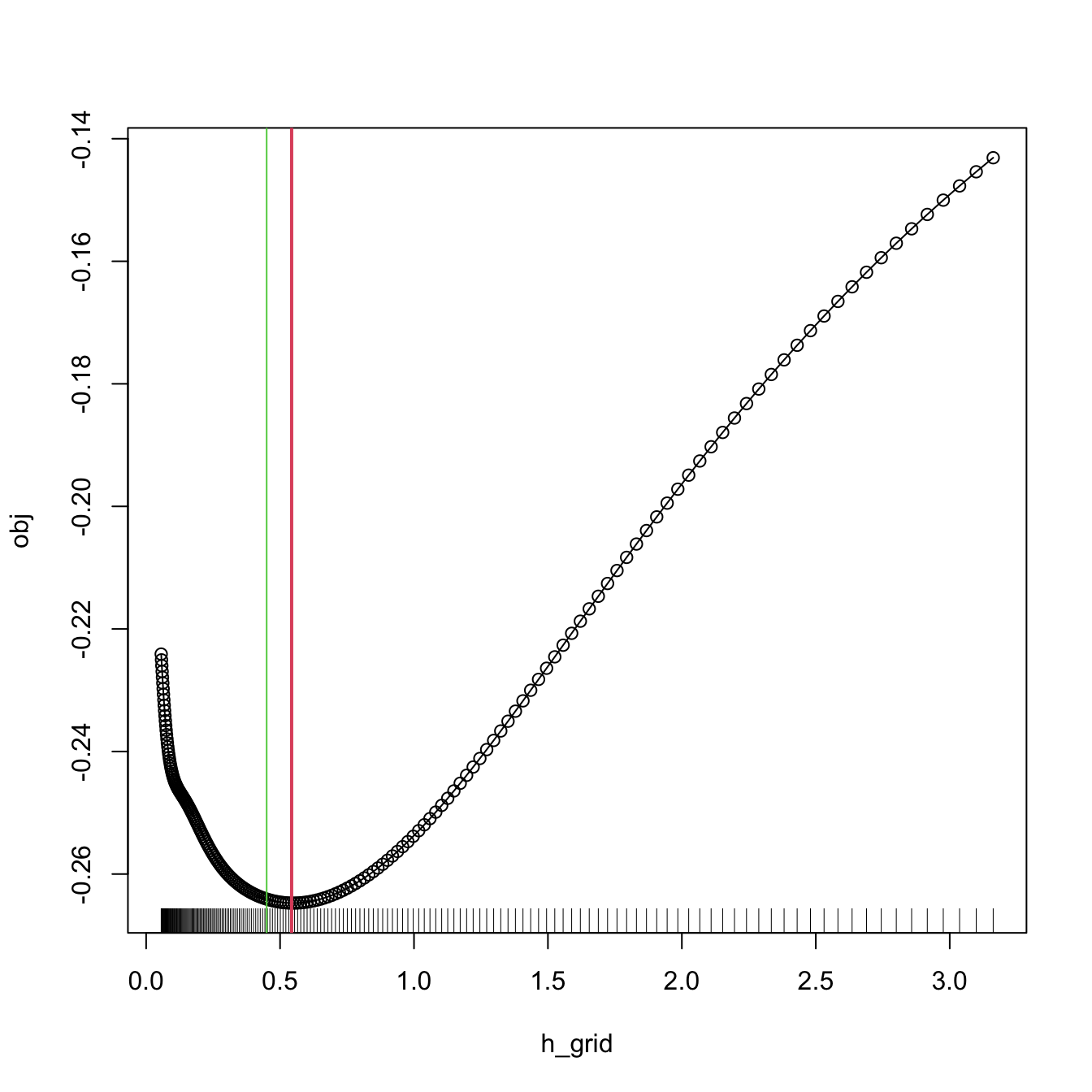

$LSCV curve evaluated for a grid of bandwidths, with a clear global minimum corresponding to $\hat{h}_\mathrm{LSCV}.$$

Figure 2.9: LSCV curve evaluated for a grid of bandwidths, with a clear global minimum corresponding to $\hat{h}_\mathrm{LSCV}.$

The next cross-validation selector is based on Biased Cross-Validation (BCV). The BCV selector presents a hybrid strategy that combines plug-in and cross-validation ideas. It starts by considering the AMISE expression in (2.23)

\[\begin{align*} \mathrm{AMISE}[\hat{f}(\cdot;h)]=\frac{1}{4}\mu^2_2(K)R(f'')h^4+\frac{R(K)}{nh} \end{align*}\]

and then plugs-in an estimate for $R(f'')$ based on a modification of $R(\hat{f}{}''(\cdot;h)).$ The modification is

\[\begin{align} \widetilde{R(f'')}:=&\,R(\hat{f}{}''(\cdot;h))-\frac{R(K'')}{nh^5}\nonumber\\ =&\,\frac{1}{n^2}\sum_{i=1}^n\sum_{\substack{j=1\\j\neq i}}^n(K_h''*K_h'')(X_i-X_j)\tag{2.30}, \end{align}\]

a leave-out-diagonals estimate of $R(f'').$ It is designed to reduce the bias of $R(\hat{f}{}''(\cdot;h)),$ since $\mathbb{E}\big[R(\hat{f}{}''(\cdot;h))\big]=R(f'')+\frac{R(K'')}{nh^5}+O(h^2)$ (Scott and Terrell 1987). Plugging (2.30) into the AMISE expression yields the BCV objective function and the BCV bandwidth selector:

\[\begin{align*} \mathrm{BCV}(h)&:=\frac{1}{4}\mu^2_2(K)\widetilde{R(f'')}h^4+\frac{R(K)}{nh},\\ \hat{h}_\mathrm{BCV}&:=\arg\mathrm{locmin}_{h>0}\mathrm{BCV}(h), \end{align*}\]

where $\arg\mathrm{locmin}_{h>0}\mathrm{BCV}(h)$ stands for the smallest local minimizer of $\mathrm{BCV}(h).$ The reason for considering the local minimum is that, by design, $\mathrm{BCV}(h)\to0$ as $h\to\infty$ for fixed $n$: $\widetilde{R(f'')}\to0,$ at a faster rate than $O(h^{-4}).$ Therefore, when minimizing $\mathrm{BCV}(h),$ some care is required, as one is actually interested in obtaining the smallest local minimizer. Consequently, bandwidth grids with an upper extreme that is too large⁴⁸ are to be avoided, as these will miss the local minimum in favor of the global one at $h\to\infty.$

The most appealing property of $\hat{h}_\mathrm{BCV}$ is that it has a considerably smaller variance than $\hat{h}_\mathrm{LSCV}.$ This reduction in variance comes at the price of an increased bias, which tends to make $\hat{h}_\mathrm{BCV}$ larger than $h_\mathrm{MISE}.$

$\hat{h}_{\mathrm{BCV}}$ is implemented in R through the function bw.bcv. Again, bw.bcv uses R’s optimize so the bw.bcv.mod function is presented to have better guarantees on finding the first local minimum. Quite some care is needed with the range of bandwidth grid, though, to avoid the global minimum for large bandwidths.

# Data
set.seed(123456)
x <- rnorm(100)

# BCV gives a warning
bw.bcv(x = x)
## [1] 0.4500924

# Extend search interval
args(bw.bcv)
## function (x, nb = 1000L, lower = 0.1 * hmax, upper = hmax, tol = 0.1 * 
##     lower) 
## NULL
bw.bcv(x = x, lower = 0.01, upper = 1)
## [1] 0.5070129

# bw.bcv.mod replaces the optimization routine of bw.bcv with an exhaustive
# search on "h_grid" (chosen adaptatively from the sample) and optionally
# plots the BCV curve with "plot_cv"
bw.bcv.mod <- function(x, nb = 1000L,
                       h_grid = 10^seq(-3, log10(1.2 * sd(x) *
                                                   length(x)^(-1/5)), l = 200),
                       plot_cv = FALSE) {
  if ((n <- length(x)) < 2L)
    stop("need at least 2 data points")
  n <- as.integer(n)
  if (is.na(n))
    stop("invalid length(x)")
  if (!is.numeric(x))
    stop("invalid 'x'")
  nb <- as.integer(nb)
  if (is.na(nb) || nb <= 0L)
    stop("invalid 'nb'")
  storage.mode(x) <- "double"
  hmax <- 1.144 * sqrt(var(x)) * n^(-1/5)
  Z <- .Call(stats:::C_bw_den, nb, x)
  d <- Z[[1L]]
  cnt <- Z[[2L]]
  fbcv <- function(h) .Call(stats:::C_bw_bcv, n, d, cnt, h)
  ## Original code
  # h <- optimize(fbcv, c(lower, upper), tol = tol)$minimum
  # if (h < lower + tol | h > upper - tol)
  #   warning("minimum occurred at one end of the range")
  ## Modification
  obj <- sapply(h_grid, function(h) fbcv(h))
  h <- h_grid[which.min(obj)]
  if (h %in% range(h_grid))
    warning("minimum occurred at one end of h_grid")
  if (plot_cv) {
    plot(h_grid, obj, type = "o")
    rug(h_grid)
    abline(v = h, col = 2, lwd = 2)
  }
  h
}

# Compute the bandwidth and plot the BCV curve
bw.bcv.mod(x = x, plot_cv = TRUE, h_grid = 10^seq(-1.25, 0.5, l = 200))
## [1] 0.5111433

# We can compare with the default bw.bcv output
abline(v = bw.bcv(x = x), col = 3)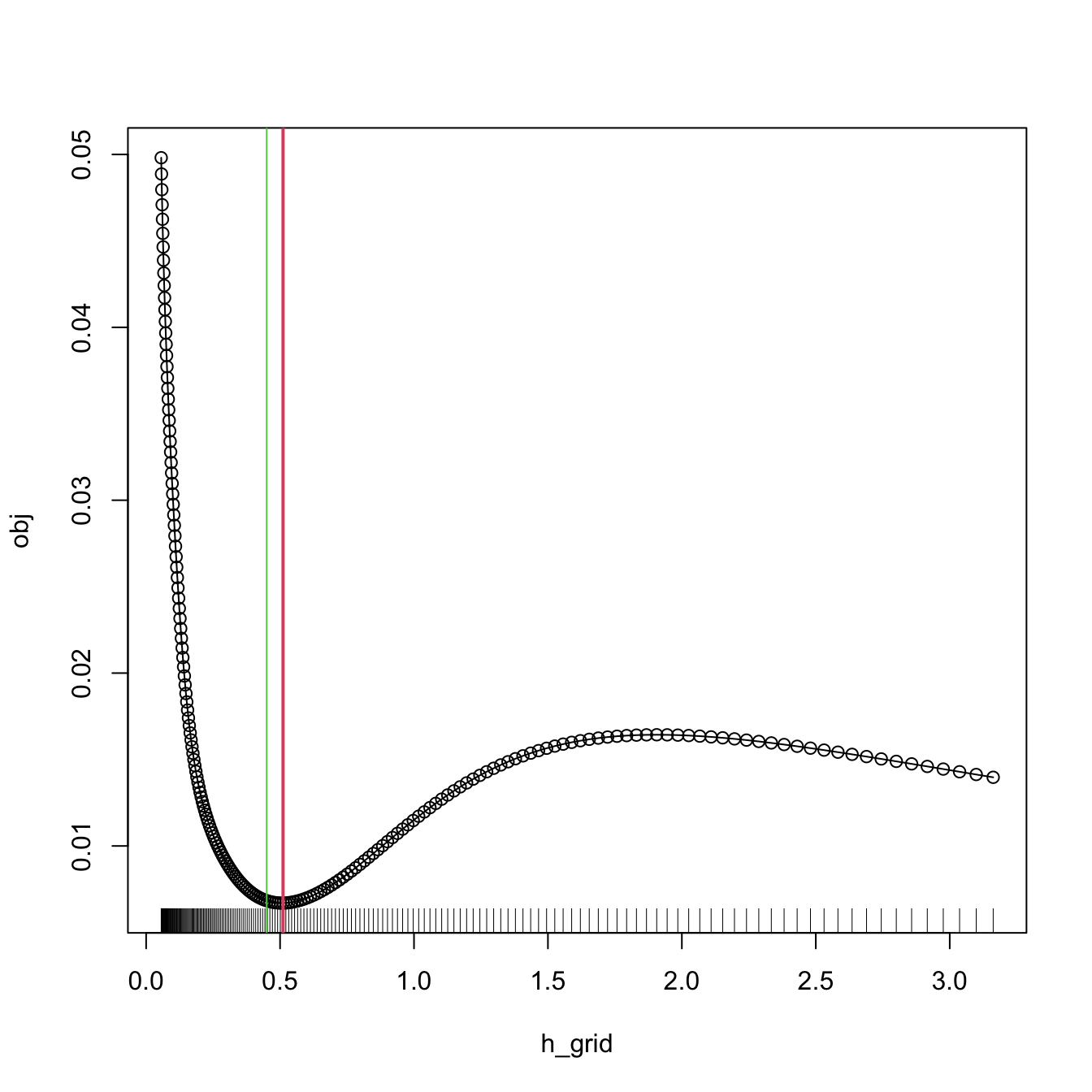

$BCV curve evaluated for a grid of bandwidths, with a clear local minimum corresponding to $\hat{h}_\mathrm{BCV}.$ Observe the decreasing pattern when $h\to\infty.$$

Figure 2.10: BCV curve evaluated for a grid of bandwidths, with a clear local minimum corresponding to $\hat{h}_\mathrm{BCV}.$ Observe the decreasing pattern when $h\to\infty.$

2.4.3 Comparison of bandwidth selectors

Next, we state some insights from the convergence results of the DPI, LSCV, and BCV selectors. All of them are based on results of the kind

\[\begin{align} n^\nu(\hat{h}/h_\mathrm{MISE}-1)\stackrel{d}{\longrightarrow}\mathcal{N}(0,\sigma^2),\tag{2.31} \end{align}\]

where $\sigma^2$ depends on $K$ and $f$ only, and measures how variable the selector is. The rate $n^\nu$ serves to quantify how fast⁴⁹ the relative error $\hat{h}/h_\mathrm{MISE}-1$ decreases (the larger the $\nu,$ the faster the convergence).

Under certain regularity conditions, we have:

$n^{1/10}(\hat{h}_\mathrm{LSCV}/h_\mathrm{MISE}-1)\stackrel{d}{\longrightarrow}\mathcal{N}(0,\sigma_\mathrm{LSCV}^2)$ and $n^{1/10}(\hat{h}_\mathrm{BCV}/h_\mathrm{MISE}-1)\stackrel{d}{\longrightarrow}\mathcal{N}(0,\sigma_\mathrm{BCV}^2).$ Both cross-validation selectors have a slow rate of convergence.⁵⁰ Inspection of the variances of both selectors reveals that, for the normal kernel, $\sigma_\mathrm{LSCV}^2/\sigma_\mathrm{BCV}^2\approx 15.7.$ Therefore, LSCV is considerably more variable than BCV.
$n^{5/14}(\hat{h}_\mathrm{DPI}/h_\mathrm{MISE}-1)\stackrel{d}{\longrightarrow}\mathcal{N}(0,\sigma_\mathrm{DPI}^2).$ Thus, the DPI selector has a convergence rate much faster than the cross-validation selectors. There is an appealing explanation for this phenomenon. Recall that $\hat{h}_\mathrm{BCV}$ minimizes the slightly modified version of $\mathrm{BCV}(h)$ given by

\[\begin{align*} \frac{1}{4}\mu_2^2(K)\tilde\psi_4(h)h^4+\frac{R(K)}{nh} \end{align*}\]

and

\[\begin{align*} \tilde\psi_4(h):=&\frac{1}{n(n-1)}\sum_{i=1}^n\sum_{\substack{j=1\\j\neq i}}^n(K_h''*K_h'')(X_i-X_j)\nonumber\\ =&\frac{n}{n-1}\widetilde{R(f'')}. \end{align*}\]

$\tilde\psi_4$ is a leave-out-diagonals estimate of $\psi_4.$ Despite being different from $\hat\psi_4,$ it serves for building a DPI analogous to BCV that points towards the precise fact that drags down the performance of BCV. The modified version of the DPI minimizes

\[\begin{align*} \frac{1}{4}\mu_2^2(K)\tilde\psi_4(g)h^4+\frac{R(K)}{nh}, \end{align*}\]

where $g$ is independent of $h.$ The two methods differ in the way $g$ is chosen: BCV sets $g=h$ and the modified DPI looks for the best $g$ in terms of the $\mathrm{AMSE}[\tilde\psi_4(g)].$ It can be seen that $g_\mathrm{AMSE}=O(n^{-2/13}),$ whereas the $h$ used in BCV is asymptotically $O(n^{-1/5}).$ This suboptimality on the choice of $g$ is the reason for the asymptotic deficiency of BCV.

We now focus on exploring the empirical performance of bandwidth selectors. The workhorse for doing that is simulation. A popular collection of simulation scenarios was given by Marron and Wand (1992) and is conveniently available through the package nor1mix. This collection is formed by normal $m$-mixtures of the form

\[\begin{align} f(x;\boldsymbol{\mu},\boldsymbol{\sigma},\mathbf{w}):&=\sum_{j=1}^m w_j\phi_{\sigma_j}(x-\mu_j), \tag{2.32} \end{align}\]

where $w_j\geq0,$ $j=1,\ldots,m$ and $\sum_{j=1}^m w_j=1.$ Densities of this form are especially attractive since they allow for arbitrary flexibility and, if the normal kernel is employed, they allow for explicit and exact MISE expressions:

\[\begin{align} \begin{split} \mathrm{MISE}_m[\hat{f}(\cdot;h)]&=(2\sqrt{\pi}nh)^{-1}+\mathbf{w}^\top\{(1-n^{-1})\boldsymbol{\Omega}_2-2\boldsymbol{\Omega}_1+\boldsymbol{\Omega}_0\}\mathbf{w},\\ (\boldsymbol{\Omega}_a)_{ij}&=\phi_{(ah^2+\sigma_i^2+\sigma_j^2)^{1/2}}(\mu_i-\mu_j),\quad i,j=1,\ldots,m. \end{split} \tag{2.33} \end{align}\]

These exact MISE expressions are highly convenient for computing $h_\mathrm{MISE},$ as defined in (2.22), by minimizing (2.33) numerically.

# Available models
?nor1mix::MarronWand

# Simulating
samp <- nor1mix::rnorMix(n = 500, obj = nor1mix::MW.nm9)
# MW object in the second argument
hist(samp, freq = FALSE)

# Density evaluation
x <- seq(-4, 4, length.out = 400)
lines(x, nor1mix::dnorMix(x = x, obj = nor1mix::MW.nm9), col = 2)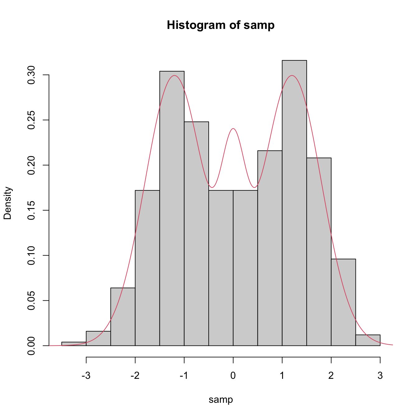


# Plot a MW object directly
# A normal with the same mean and variance is plotted in dashed lines --
# you can remove it with argument p.norm = FALSE
par(mfrow = c(2, 2))
plot(nor1mix::MW.nm5)
plot(nor1mix::MW.nm7)
plot(nor1mix::MW.nm10)
plot(nor1mix::MW.nm12)
lines(nor1mix::MW.nm7, col = 2) # Also possible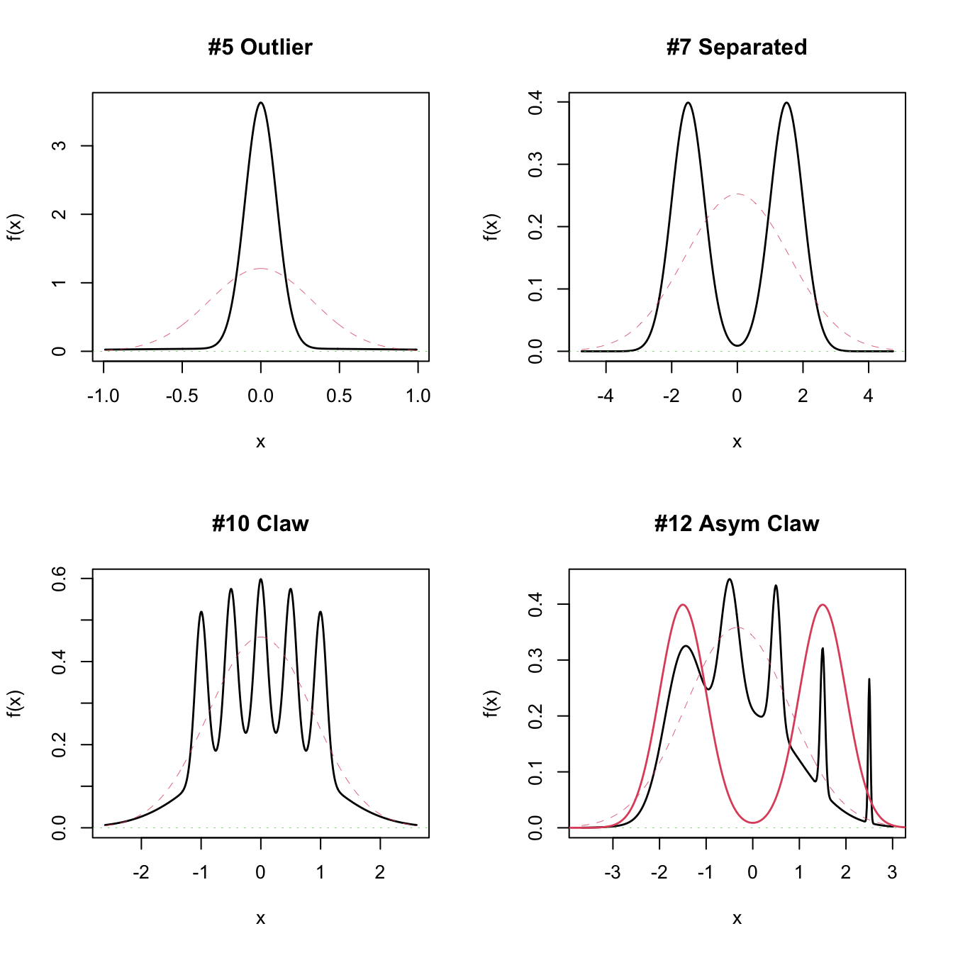

Exercise 2.18 Implement the $h_\mathrm{MISE}$ using (2.22) and (2.33) for model nor1mix::MW.nm6. Then, compute by Monte Carlo the densities of $\hat{h}_\mathrm{DPI}/h_\mathrm{MISE}-1,$ $\hat{h}_\mathrm{LSCV}/h_\mathrm{MISE}-1,$ and $\hat{h}_\mathrm{BCV}/h_\mathrm{MISE}-1.$ Compare them for $n=100,200,500.$ Describe in detail the results and the major takeaways in relation to the properties of the bandwidth selectors.

Exercise 2.19 Compare the MISE and AMISE criteria in three densities in nor1mix of your choice. To that purpose, code (2.33) and the AMISE expression for the normal kernel, and compare the two error curves. Compare them for $n=100,200,500,$ adding a vertical line to represent the $h_\mathrm{MISE}$ and $h_\mathrm{AMISE}$ bandwidths. Describe in detail the results and the major takeaways in relation to using $h_\mathrm{AMISE}$ as a proxy for $h_\mathrm{MISE}$.

A key practical issue that emerges after discussing several bandwidth selectors is the following:

Which bandwidth selector is the most adequate for a given dataset?

Unfortunately, there is no simple and universal answer to this question. There are, however, a series of useful facts and suggestions:

Trying several selectors and inspecting the results may help to determine which one is estimating the density better.
The DPI selector has a convergence rate much faster than the cross-validation selectors. Therefore, in theory it is expected to perform better than LSCV and BCV. For this reason, it tends to be among the preferred bandwidth selectors in the literature.
Cross-validatory selectors may be better suited for highly non-normal and rough densities, in which plug-in selectors may end up oversmoothing.
LSCV tends to be considerably more variable than BCV.
The RT is a quick, simple, and inexpensive selector. However, it tends to give bandwidths that are too large for non-normal-like data.

Figure 2.11 presents a visualization of the performance of the kde with different bandwidth selectors, carried out in the family of mixtures by Marron and Wand (1992).

Figure 2.11: Performance comparison of bandwidth selectors. The RT, DPI, LSCV, and BCV are computed for each sample for a normal mixture density. For each sample, the animation computes the ISEs of the selectors and sorts them from best to worst. Changing the scenarios gives insight into the adequacy of each selector to hard- and simple-to-estimate densities. Application available here.

2.5 Practical issues

In this section we discuss several practical issues for kernel density estimation.

2.5.1 Boundary issues and transformations

In Section 2.3 we assumed certain regularity conditions for $f.$ Assumption A1 stated that $f$ should be twice continuously differentiable (on $\mathbb{R}$!). It is simple to think a counterexample to that: take any density with a support with boundary, for example a $\mathcal{LN}(0,1)$ in $(0,\infty),$ as seen below. The kde will run into trouble!

# Sample from a LN(0, 1)
set.seed(123456)
samp <- rlnorm(n = 500)

# kde and density
plot(density(samp), ylim = c(0, 0.8))
curve(dlnorm(x), from = -2, to = 10, n = 500, col = 2, add = TRUE)
rug(samp)

What is happening is clear: the kde is spreading probability mass outside the support of $\mathcal{LN}(0,1),$ because the kernels are functions defined in $\mathbb{R}.$ Since the kde places probability mass at negative values, it takes it from the positive side, resulting in a severe negative bias about the right-hand side of $0.$ As a consequence, the kde does not integrate to one in the support of the data. No matter what the sample size considered is, the kde will always have a negative bias of $O(h)$ at the boundary, instead of the standard $O(h^2).$

A simple approach to deal with the boundary bias is to map a non-real-supported density $f$ into a real-supported density $g,$ which is simpler to estimate, by means of a transformation $t$:

\[\begin{align*} f(x)=g(t(x))t'(x). \end{align*}\]

The transformation kde is obtained by replacing $g$ with the usual kde, but acting on the transformed data $t(X_1),\ldots,t(X_n)$:

\[\begin{align} \hat{f}_\mathrm{T}(x;h,t):=\frac{1}{n}\sum_{i=1}^nK_h(t(x)-t(X_i))t'(x). \tag{2.34} \end{align}\]

Note that $h$ is in the scale of $t(X_i),$ not $X_i.$ Hence, another benefit of this approach, in addition to its simplicity, is that bandwidth selection can be done transparently⁵¹ in terms of the already discussed bandwidth selectors: select a bandwidth from $t(X_1),\ldots,t(X_n)$ and use it in (2.34). A table with some common transformations⁵² is the following.

Transform.	Data in	$t(x)$	$t'(x)$
Log	$(a,\infty)$	$\log(x-a)$	$\frac{1}{x-a}$
Probit	$(a,b)$	$\Phi^{-1}\left(\frac{x-a}{b-a}\right)$	${(b-a)\phi\left(\frac{\Phi^{-1}(x)-a}{b-a}\right)^{-1}}$
Shifted power	$(-\lambda_1,\infty)$ (data skewed)	${(x+\lambda_1)^{\lambda_2}\mathrm{sign}(\lambda_2)}$ if $\lambda_2\neq0$	${\lambda_2(x+\lambda_1)^{\lambda_2-1}\mathrm{sign}(\lambda_2)}$ if $\lambda_2\neq0$

Figure 2.12: Construction of the transformation kde for the log and probit transformations. The left panel shows the kde (2.7) applied to the transformed data. The right plot shows the transformed kde (2.34) applied to the original data. Application available here.

The code below illustrates how to compute a transformation kde in practice from density.

# kde with log-transformed data
kde <- density(log(samp))
plot(kde, main = "Kde of transformed data")
rug(log(samp))


# Careful: kde$x is in the reals!
range(kde$x)
## [1] -4.542984  3.456035

# Untransform kde$x so the grid is in (0, infty)
kde_transf <- kde
kde_transf$x <- exp(kde_transf$x)

# Transform the density using the chain rule
kde_transf$y <- kde_transf$y * 1 / kde_transf$x

# Transformed kde
plot(kde_transf, main = "Transformed kde", xlim = c(0, 15))
curve(dlnorm(x), col = 2, add = TRUE, n = 500)
rug(samp)

Exercise 2.20 Consider the data given by set.seed(12345); x <- rbeta(n = 500, shape1 = 2, shape2 = 2). Compute:

The untransformed kde employing the DPI and LSCV selectors. Overlay the true density.
The transformed kde employing a probit transformation and using the DPI and LSCV selectors on the transformed data.

Exercise 2.21 (Exercise 2.23 in Wand and Jones (1995)) Show that the bias and variance for the transformation kde (2.34) are

\[\begin{align*} \mathrm{Bias}[\hat{f}_\mathrm{T}(x;h,t)]&=\frac{1}{2}\mu_2(K)g''(t(x))t'(x)h^2+o(h^2),\\ \mathbb{V}\mathrm{ar}[\hat{f}_\mathrm{T}(x;h,t)]&=\frac{R(K)}{nh}g(t(x))t'(x)^2+o((nh)^{-1}), \end{align*}\]

where $g$ is the density of $t(X).$

Exercise 2.22 Using the results from Exercise 2.21, prove that

\[\begin{align*} \mathrm{AMISE}[\hat{f}_\mathrm{T}(\cdot;h,t)]=&\,\frac{1}{4}\mu_2^2(K)\int (g''(x))^2t'(t^{-1}(x))\,\mathrm{d}xh^4\\ &+\frac{R(K)}{nh}\mathbb{E}[t'(X)], \end{align*}\]

where $g$ is the density of $t(X).$

2.5.2 Sampling

Sampling a kde is relatively straightforward. The trick is to recall

\[\begin{align*} \hat{f}(x;h)=\frac{1}{n}\sum_{i=1}^nK_h(x-X_i) \end{align*}\]

as a mixture density made of $n$ mixture components in which each of them is sampled independently. The only part that might require special treatment is sampling from the density $K,$ although R contains specific sampling functions for the most popular kernels.

The algorithm for sampling $N$ points goes as follows:

Choose $i\in\{1,\ldots,n\}$ at random.
Sample from $K_h(\cdot-X_i)=\frac{1}{h}K\left(\frac{\cdot-X_i}{h}\right).$
Repeat the previous steps $N$ times.

Let’s see a quick example.

# Sample the claw
n <- 100
set.seed(23456)
samp <- nor1mix::rnorMix(n = n, obj = nor1mix::MW.nm10)

# Kde
h <- 0.1
plot(density(samp, bw = h), main = "", col = 4)

# # Naive sampling algorithm
# N <- 1e6
# samp_kde <- numeric(N)
# for (k in 1:N) {
#
#   i <- sample(x = 1:n, size = 1)
#   samp_kde[k] <- rnorm(n = 1, mean = samp[i], sd = h)
#
# }

# Sample N points from the kde
N <- 1e6
i <- sample(x = n, size = N, replace = TRUE)
samp_kde <- rnorm(N, mean = samp[i], sd = h)

# Add kde of the sampled kde -- almost equal
lines(density(samp_kde), col = 3)
legend("topright", legend = c("Kde", "Kde of sampled kde"),
       lwd = 2, col = 4:3)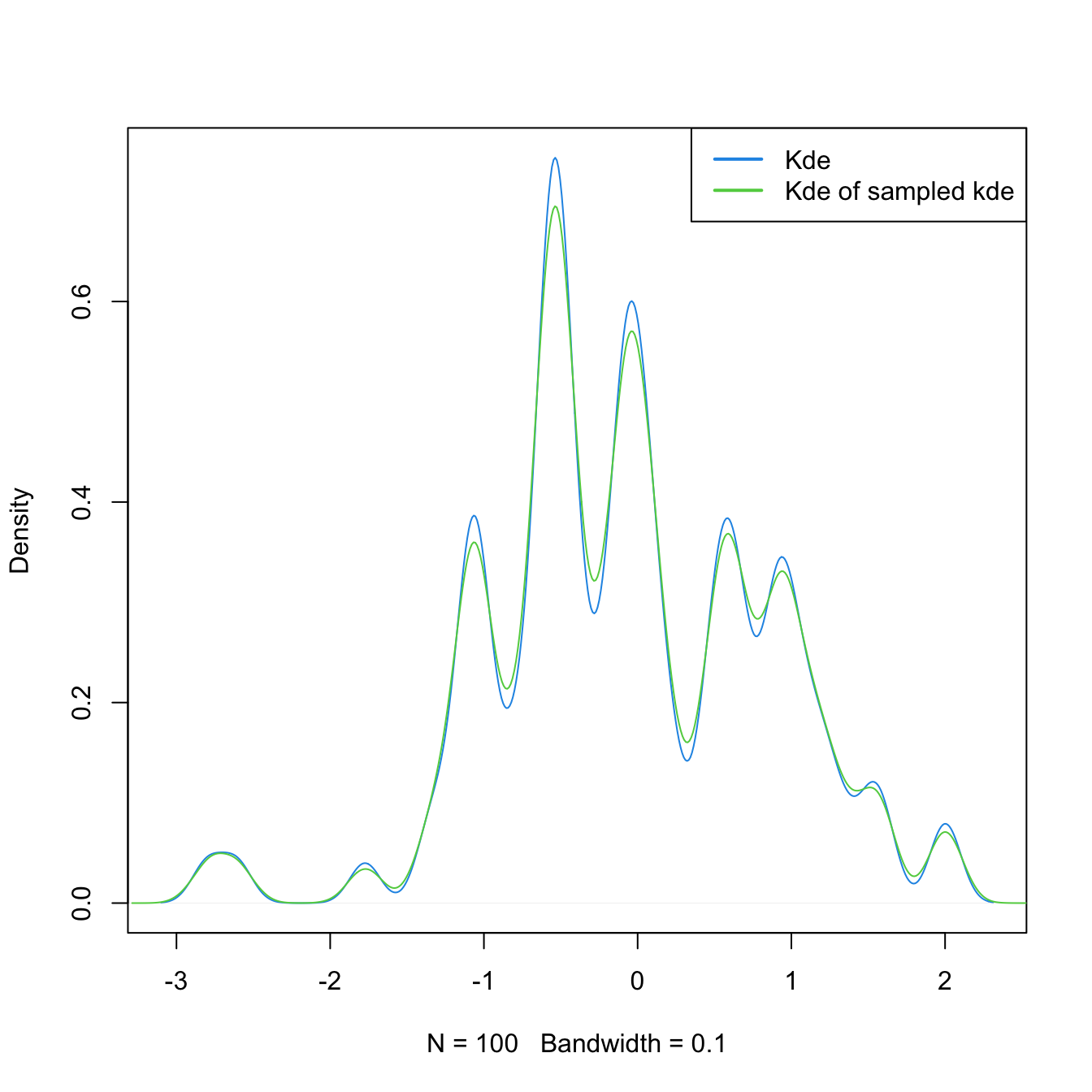

Exercise 2.23 Sample data points from the kde of iris$Petal.Width that is computed with the NS selector.

Exercise 2.24 The dataset sunspot.year contains the yearly numbers of sunspots from 1700 to 1988 (rounded to one digit). Employing a log-transformed kde with DPI bandwidth, sample new sunspots observations. Check by simulation that the sampling is done appropriately by comparing the log-transformed kde of the sampled data with the original kde.

2.6 Kernel density estimation with `ks`

The density function in R presents certain limitations, such as the impossibility of evaluating the kde at arbitrary points, the unavailability of built-in transformations, and the lack of a multivariate extension. The ks package (Duong 2020) delivers the ks::kde function, providing these and other functionalities. It will be the workhorse for carrying out multivariate kde (Section 3.1). The only drawback of ks::kde to be aware of is that it only considers normal kernels – though these are by far the most popular.

The following chunk of code shows that density and ks::kde give the same outputs. It also presents some of the extra flexibility on the evaluation that ks::kde provides.

# Sample
n <- 5
set.seed(123456)
samp_t <- rt(n, df = 2)

# Comparison: same output and same parametrization for bandwidth
bw <- 0.75
plot(kde <- ks::kde(x = samp_t, h = bw), lwd = 3) # ?ks::plot.kde for options
lines(density(x = samp_t, bw = bw), col = 2)
# Beware: there is no lines() method for ks::kde objects

# The default h is the DPI obtained by ks::hpi
kde <- ks::kde(x = samp_t)

# Manual plot -- recall $eval.points and $estimate
lines(kde$eval.points, kde$estimate, col = 4)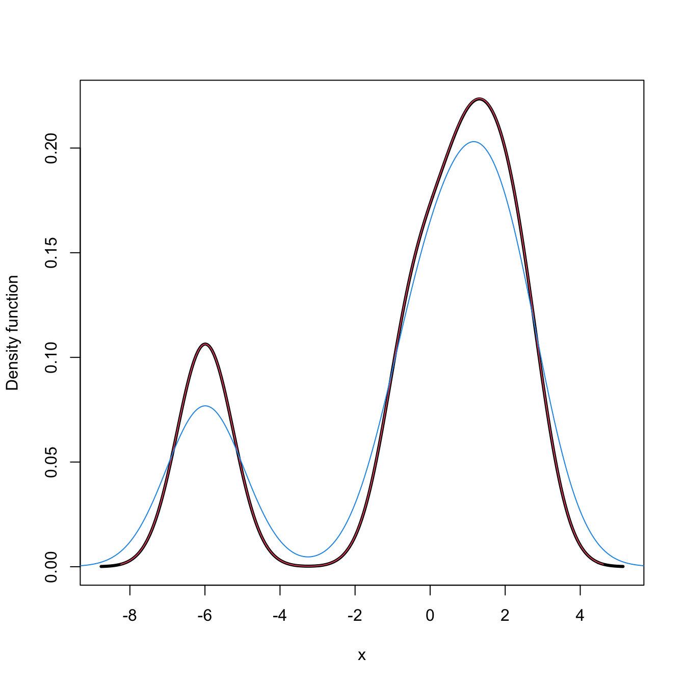


# Evaluating the kde at specific points, e.g., the first 2 sample points
ks::kde(x = samp_t, h = bw, eval.points = samp_t[1:2])
## $x
## [1]  1.4650470 -0.4971902  0.6701367  2.3647267 -5.9918352
## 
## $eval.points
## [1]  1.4650470 -0.4971902
## 
## $estimate
## [1] 0.2223029 0.1416113
## 
## $h
## [1] 0.75
## 
## $H
## [1] 0.5625
## 
## $gridtype
## [1] "linear"
## 
## $gridded
## [1] TRUE
## 
## $binned
## [1] TRUE
## 
## $names
## [1] "x"
## 
## $w
## [1] 1 1 1 1 1
## 
## $type
## [1] "kde"
## 
## attr(,"class")
## [1] "kde"

# By default ks::kde() computes the *binned* kde (much faster) and then employs
# an interpolation to evaluate the kde at the given grid; if the exact kde is
# desired, this can be specified with binned = FALSE
ks::kde(x = samp_t, h = bw, eval.points = samp_t[1:2], binned = FALSE)
## $x
## [1]  1.4650470 -0.4971902  0.6701367  2.3647267 -5.9918352
## 
## $eval.points
## [1]  1.4650470 -0.4971902
## 
## $estimate
## [1] 0.2223316 0.1416132
## 
## $h
## [1] 0.75
## 
## $H
## [1] 0.5625
## 
## $gridded
## [1] FALSE
## 
## $binned
## [1] FALSE
## 
## $names
## [1] "x"
## 
## $w
## [1] 1 1 1 1 1
## 
## $type
## [1] "kde"
## 
## attr(,"class")
## [1] "kde"

# Changing the size of the evaluation grid
length(ks::kde(x = samp_t, h = bw, gridsize = 1e3)$estimate)
## [1] 1000

The computation of log-transformed kde is straightforward using the positive and adj.positive arguments.

# Sample from a LN(0, 1)
set.seed(123456)
samp_ln <- rlnorm(n = 200)

# Log-kde without shifting
a <- seq(0.1, 2, by = 0.4) # Sequence of shifts
col <- viridis::viridis(length(a) + 1)
plot(ks::kde(x = samp_ln, positive = TRUE), col = col[1],
     main = "Log-transformed kde and the effect of adj.positive",
     xlim = c(0, 7.5), ylim = c(0, 0.75))
# If h is not provided, then ks::hpi() is called on the transformed data

# Shifting: larger a increases the bias
for (i in seq_along(a)) {
  plot(ks::kde(x = samp_ln, positive = TRUE, adj.positive = a[i]),
       add = TRUE, col = col[i + 1])
}
curve(dlnorm(x), col = 2, add = TRUE, n = 500)
rug(samp_ln)
legend("topright", legend = c("True density", paste("adj.positive =", c(0, a))),
       col = c(2, col), lwd = 2)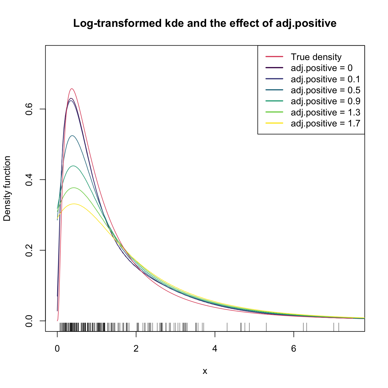

Finally, sampling from the kde and log-transformed kde is easily achieved by the use of ks::rkde.

# Untransformed kde
plot(kde <- ks::kde(x = log(samp_ln)), col = 4)
samp_kde <- ks::rkde(n = 5e4, fhat = kde)
plot(ks::kde(x = samp_kde), add = TRUE, col = 3)
legend("topright", legend = c("Kde", "Kde of sampled kde"),
       lwd = 2, col = 3:4)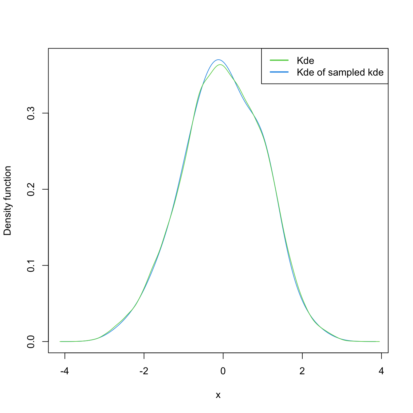


# Transformed kde
plot(kde_transf <- ks::kde(x = samp_ln, positive = TRUE), col = 4)
samp_kde_transf <- ks::rkde(n = 5e4, fhat = kde_transf, positive = TRUE)
plot(ks::kde(x = samp_kde_transf), add = TRUE, col = 3)
legend("topright", legend = c("Kde", "Kde of sampled kde"),
       lwd = 2, col = 3:4)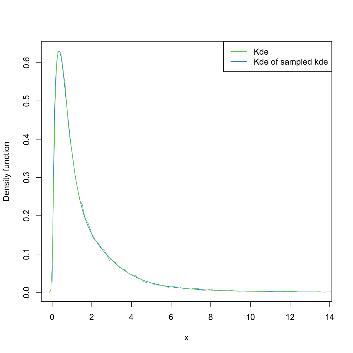

Exercise 2.25 Consider the MNIST dataset in the MNIST-tSNE.RData file. It contains the first $60,000$ images of the MNIST database. Each observation is a grayscale image made of $28\times 28$ pixels that is recorded as a vector of length $28^2=784$ by concatenating the pixel columns. The entries of these vectors are numbers in $[0,1]$ indicating the level of grayness of the pixel: $0$ for white, $1$ for black. These vectorized images are stored in the $60,000\times 784$ matrix in MNIST$x. The $0$–$9$ labels of the digits are stored in MNIST$labels.

Compute the average gray level, av_gray_one, for each image of the digit “1”.
Compute and plot the kde of av_gray_one. Consider taking into account that it is a positive variable.
Overlay the lognormal distribution density, with parameters estimated by maximum likelihood (use MASS::fitdistr).
Repeat part c for the Weibull density.
Which parametric model seems more adequate?

References

Devroye, L., and L. Györfi. 1985. Nonparametric Density Estimation. Wiley Series in Probability and Mathematical Statistics. New York: John Wiley & Sons. https://www.szit.bme.hu/~gyorfi/L1bookBW.pdf.

Duong, T. 2020. ks: Kernel Smoothing. https://CRAN.R-project.org/package=ks.

Marron, J. S., and M. P. Wand. 1992. “Exact Mean Integrated Squared Error.” The Annals of Statistics 20 (2): 712–36. https://doi.org/10.1214/aos/1176348653.

Parzen, E. 1962. “On Estimation of a Probability Density Function and Mode.” Annals of Mathematical Statistics 33 (3): 1065–76. https://doi.org/10.1214/aoms/1177704472.

Rosenblatt, M. 1956. “Remarks on Some Nonparametric Estimates of a Density Function.” Annals of Mathematical Statistics 27 (3): 832–37. https://doi.org/10.1214/aoms/1177728190.

Scott, D. W. 2015. Multivariate Density Estimation. Second. Wiley Series in Probability and Statistics. Hoboken: John Wiley & Sons. https://doi.org/10.1002/9781118575574.

Scott, D. W., and G. R. Terrell. 1987. “Biased and Unbiased Cross-Validation in Density Estimation.” Journal of the American Statistical Association 82 (400): 1131–46. https://doi.org/10.1080/01621459.1987.10478550.

Sheather, S. J., and M. C. Jones. 1991. “A Reliable Data-Based Bandwidth Selection Method for Kernel Density Estimation.” Journal of the Royal Statistical Society, Series B (Methodological) 53 (3): 683–90. https://doi.org/10.1111/j.2517-6161.1991.tb01857.x.

Wand, M. P., and M. C. Jones. 1995. Kernel Smoothing. Vol. 60. Monographs on Statistics and Applied Probability. London: Chapman & Hall. https://doi.org/10.1201/b14876.

Another example is the $p$-quantile $x_p:=F^{(-1)}(p),$ where $F^{(-1)}(u):=\inf\{x\in\mathbb{R}:F(x)\geq u\}$ is the pseudo-inverse of the cdf $F.$ Then, $x_p$ can be estimated by the sample $p$-quantile $\hat{x}_p:=F_n^{(-1)}(p).$↩︎
Is not even continuous!↩︎
Note that we estimate $f(x)$ by means of an estimate for $f(x_0),$ where $x$ is at most $h>0$ units above $x_0.$ Thus, we do not estimate directly $f(x)$ with the histogram.↩︎
Recall that, with this standardization, we approach the probability density concept.↩︎
Note that it is key that the $\{B_k\}$ are deterministic (and not sample-dependent) for this result to hold.↩︎
This is an important point. Notice also that this $k$ depends on $h$ because $t_k=t_0+kh,$ therefore the $k$ for which $x\in\lbrack t_k,t_{k+1})$ will change when, for example, $h\to0.$↩︎
Because $x\in \lbrack t_k,t_{k+1})$ with $k$ changing as $h\to0$ (see the previous footnote) and the interval ends up collapsing in $x,$ so any point in $\lbrack t_k,t_{k+1})$ converges to $x.$↩︎
The motivation for this terminology will be apparent in Section 2.2.↩︎
Or, in other words, if $h^{-1}=o(n),$ i.e., if $h^{-1}$ grows more slowly than $n$ does.↩︎
Why so?↩︎
In greater generality, the kernel $K$ might only be assumed to be an integrable function with unit integral.↩︎
Also known as the Parzen–Rosenblatt estimator to honor the proposals by Parzen (1962) and Rosenblatt (1956).↩︎
Although the efficiency of the normal kernel, with respect to the Epanechnikov kernel, is roughly $0.95.$↩︎
Precisely, the rule-of-thumb given by bw.nrd.↩︎
The variance, since $\int zK(z)\,\mathrm{d}z=0$ because the kernel is symmetric with respect to zero.↩︎
Finite-sample results might be either analytically infeasible or dependent on simulation studies that are necessarily limited in their scope.↩︎
This assumption requires certain smoothness of the pdf, allowing thus for Taylor expansions to be performed on $f.$↩︎
Mild assumption that makes the first term of the Taylor expansion of $f$ negligible and the second one bounded.↩︎
The key assumption for reducing the bias and variance of $\hat{f}(\cdot;h)$ simultaneously.↩︎
$h=h_n$ always depends on $n$ from now on, although the subscript is dropped for ease of notation.↩︎
Since $\mathrm{Bias}[\hat{f}(x;h)]=(K_h*f)(x)-f(x)\neq 0.$ An example of this bias is given in Section A.↩︎
The variance of an unweighted mean is reduced by a factor $n^{-1}$ when $n$ observations are employed. For computing $\hat{f}(x;h),$ $n$ observations are used but in a weighted fashion that roughly amounts to considering $nh$ unweighted observations.↩︎
That is, towards the random variable that always takes the value $f(x).$↩︎
This is satisfied, for example, if the kernel decreases exponentially, i.e., if $\exists\, \alpha,\,M>0: K(z)\leq e^{-\alpha|z|},\,\forall|z|>M.$↩︎
For defining $\hat g(y;h)$ we consider the transformed kde seen in Section 2.5.1.↩︎
Since $n^{-4/5}=o(n^{-2/3}).$↩︎
We only use a parametric assumption for estimating the curvature of $f$ in present $h_\mathrm{AMISE},$ not for directly estimating $f$ itself.↩︎
Not to confuse with bw.nrd0!↩︎
See Section 3.5 in Wand and Jones (1995) for full details.↩︎
Recall there is no “I”, since we are estimating a scalar, not a function.↩︎
For the rule-of-thumb selector, $\ell=0$ and we estimate $\psi_{4}$ parametrically. If $\ell=2,$ we estimate $\psi_{8}$ parametrically, which is then required for estimating $\psi_{6}$ nonparametrically.↩︎
Hence, what we are doing is “sweeping under $\ell$ nonparametric carpets” this parametric estimate on the characteristic $\psi_{\ell+4}$ of the density, ultimately required for computing the bandwidth selector.↩︎
Why so? Because $X$ is unbiased for estimating $\mathbb{E}[X].$↩︎
Long intervals containing the solution may lead to unsatisfactory termination of the search; short intervals might not contain the minimum.↩︎
The precise point at which a bandwidth is “too big” can be formalized with the maximal smoothing principle, as elaborated in Section 3.2.2 in Wand and Jones (1995).↩︎
Recall that another way of writing (2.31) is as the relative error $\frac{\hat{h}-h_\mathrm{MISE}}{h_\mathrm{MISE}}$ being asymptotically distributed as a $\mathcal{N}\left(0,\frac{\sigma^2}{n^{2\nu}}\right).$↩︎
Compare it with the $n^{1/2}$ rate of the CLT!↩︎
However, note that the optimality on selecting a bandwidth for estimating $g$ from $t(X_1),\ldots,t(X_n)$ may not translate into an optimality for estimating $f.$↩︎
If $\lambda_2\to0$ in the shifted power, then the log transformation follows with $a=-\lambda_1.$↩︎

1 Introduction

3 Kernel density estimation II

Transform.	Data in	\(t(x)\)	\(t'(x)\)
Log	\((a,\infty)\)	\(\log(x-a)\)	\(\frac{1}{x-a}\)
Probit	\((a,b)\)	\(\Phi^{-1}\left(\frac{x-a}{b-a}\right)\)	\({(b-a)\phi\left(\frac{\Phi^{-1}(x)-a}{b-a}\right)^{-1}}\)
Shifted power	\((-\lambda_1,\infty)\) (data skewed)	\({(x+\lambda_1)^{\lambda_2}\mathrm{sign}(\lambda_2)}\) if \(\lambda_2\neq0\)	\({\lambda_2(x+\lambda_1)^{\lambda_2-1}\mathrm{sign}(\lambda_2)}\) if \(\lambda_2\neq0\)