6 Nonparametric tests

This chapter overviews some well-known nonparametric hypothesis tests.¹⁹⁵ The reviewed tests are intended for different purposes, mostly related to: (i) the evaluation of the goodness-of-fit of a distribution model to a dataset; and (ii) the assessment of the relation between two random variables.

A nonparametric test evaluates a null hypothesis $H_0$ against an alternative $H_1$ without assuming any parametric model, on neither $H_0$ nor $H_1.$ Consequently, a nonparametric test is free from the overhead of evaluating a parametric assumption that one needs to conduct before applying a parametric test.¹⁹⁶ More importantly, it is quite likely that the inspection of these parametric assumptions has a negative outcome that forbids the subsequent application of a parametric test. The direct applicability and generality of nonparametric tests are the reasons for their usefulness in real-data applications.

Nonparametric tests have lower efficiency with respect to optimal parametric tests for specific parametric problems.¹⁹⁷ Statistical inference is full of instances of such parametric tests, especially within the context of normal populations.¹⁹⁸ For example, given two iid samples $X_{11},\ldots,X_{1n_1}$ and $X_{21},\ldots,X_{2n_2}$ from two normal populations $X_1\sim\mathcal{N}(\mu_1,\sigma^2)$ and $X_2\sim\mathcal{N}(\mu_2,\sigma^2),$ the test for the equality of the means,

\[\begin{align*} H_0:\mu_1=\mu_2\quad\text{vs.}\quad H_1:\mu_1\neq\mu_2, \end{align*}\]

is optimally carried out using the test statistic $T_n:=\frac{\bar{X}_1-\bar{X}_2}{S\sqrt{1/n_1+1/n_2}},$ where $S^2:=\frac{1}{n_1+n_2-2}\left(\sum_{i=1}^{n_1}(X_{1i}-\bar{X}_1)^2+\sum_{i=1}^{n_2}(X_{2i}-\bar{X}_2)^2\right)$ is the pooled sample variance. The distribution of $T_n$ under $H_0$ is $t_{n_1+n_2-2},$ which is compactly denoted by $T_n\stackrel{H_0}{\sim}t_{n_1+n_2-2}.$ For this result to hold, it is key that the two populations are indeed normally distributed, an assumption that may be unrealistic in practice. Recall that, under $H_0,$ this test states the equality of distributions of $X_1$ and $X_2.$ A nonparametric alternative therefore is the Kolmogorov–Smirnov test for two samples, to be seen in Section 6.2. It evaluates if the distributions of $X_1\sim F_1$ and $X_2\sim F_2$ are equal:

\[\begin{align*} H_0:F_1=F_2\quad\text{vs.}\quad H_1:F_1\neq F_2. \end{align*}\]

Finally, the term goodness-of-fit refers to the statistical tests that check the adequacy of a model for explaining a sample. For example, a goodness-of-fit test allows answering if a normal model is “acceptable” to describe a given sample $X_1,\ldots,X_n.$ Initially, the concept of goodness-of-fit test was proposed for distribution models, but it was later extended to regression¹⁹⁹ and other statistical models,²⁰⁰ although such extensions are not addressed in this book.

6.1 Goodness-of-fit tests for distribution models

Assume that an iid sample $X_1,\ldots,X_n$ from an arbitrary distribution $F$ is given.²⁰¹ We next address the one-sample problem of testing a statement about the unknown distribution $F.$

6.1.1 Simple hypothesis tests

We first address tests for the simple null hypothesis

\[\begin{align} H_0:F=F_0 \tag{6.1} \end{align}\]

against the most general alternative²⁰²

\[\begin{align*} H_1:F\neq F_0, \end{align*}\]

where here and henceforth “$F\neq F_0$” means that there exists at least one $x\in\mathbb{R}$ such that $F(x)\neq F_0(x),$ and $F_0$ is a pre-specified, non-data-dependent distribution model. This latter aspect is very important:

If some parameters of $F_0$ are estimated from the sample, the presented tests for (6.1) will not respect the significance level $\alpha$ for which they are constructed, and as a consequence they will be highly conservative.²⁰³

Recall that the ecdf (1.1) of $X_1,\ldots,X_n,$ $F_n(x)=\frac{1}{n}\sum_{i=1}^n1_{\{X_i\leq x\}},$ is a nonparametric estimator of $F,$ as seen in Section 1.6. Therefore, a measure of proximity of $F_n$ (driven by the sample) and $F_0$ (specified by $H_0$) will be indicative of the veracity of (6.1): a “large” distance between $F_n$ and $F_0$ evidences that $H_0$ is likely to be false.²⁰⁴ $\!\!^,$²⁰⁵

The following three well-known goodness-of-fit tests arise from the same principle: considering as the test statistic a particular type of distance between the functions $F_n$ and $F_0.$

6.1.1.1 Kolmogorov–Smirnov test

Test purpose. Given $X_1,\ldots,X_n\sim F,$ it tests $H_0: F=F_0$ vs. $H_1: F\neq F_0$ consistently against all the alternatives in $H_1.$
Statistic definition. The test statistic uses the supremum distance²⁰⁶ $\!\!^,$²⁰⁷ between $F_n$ and $F_0$:

\[\begin{align*} D_n:=\sqrt{n}\sup_{x\in\mathbb{R}} \left|F_n(x)-F_0(x)\right|. \end{align*}\]

If $H_0:F=F_0$ holds, then $D_n$ tends to be small. Conversely, when $F\neq F_0,$ larger values of $D_n$ are expected, and the test rejects $H_0$ when $D_n$ is large.
Statistic computation. The computation of $D_n$ can be efficiently achieved by realizing that the maximum difference between $F_n$ and $F_0$ happens at $x=X_i,$ for a certain $X_i$ (observe Figure 6.1). From here, sorting the sample and applying the probability transformation $F_0$ gives²⁰⁸

\[\begin{align} D_n=&\,\max(D_n^+,D_n^-),\tag{6.2}\\ D_n^+:=&\,\sqrt{n}\max_{1\leq i\leq n}\left\{\frac{i}{n}-U_{(i)}\right\},\nonumber\\ D_n^-:=&\,\sqrt{n}\max_{1\leq i\leq n}\left\{U_{(i)}-\frac{i-1}{n}\right\},\nonumber \end{align}\]

where $U_{(j)}$ stands for the $j$-th sorted $U_i:=F_0(X_i),$ $i=1,\ldots,n.$
Distribution under $H_0.$ If $H_0$ holds and $F_0$ is continuous, then $D_n$ has an asymptotic²⁰⁹ cdf given by the Kolmogorov–Smirnov’s $K$²¹⁰ function:

\[\begin{align} \lim_{n\to\infty}\mathbb{P}[D_n\leq x]=K(x):=1-2\sum_{j=1}^\infty (-1)^{j-1}e^{-2j^2x^2}.\tag{6.3} \end{align}\]
Highlights and caveats. The Kolmogorov–Smirnov test is a distribution-free test because its distribution under $H_0$ does not depend on $F_0.$ However, this is the case only if $F_0$ is continuous and the sample $X_1,\ldots,X_n$ is also continuous, i.e., if the sample has no ties.²¹¹ If these assumptions are met, then the iid sample $X_1,\ldots,X_n\stackrel{H_0}{\sim} F_0$ generates the iid sample $U_1,\ldots,U_n\stackrel{H_0}{\sim} \mathcal{U}(0,1),$ with $U_i:=F_0(X_i),$ $i=1,\ldots,n.$ As a consequence, the distribution of (6.2) does not depend on $F_0$.²¹² $\!\!^,$²¹³ If $F_0$ is not continuous or there are ties on the sample, the $K$ function is not the true asymptotic cdf. An alternative for discrete $F_0$ is given below. In case there are ties on the sample, a possibility is to slightly perturb the sample in order to remove such ties.²¹⁴
Implementation in R. For continuous data and continuous $F_0,$ the test statistic $D_n$ and the asymptotic $p$-value²¹⁵ are readily available through the ks.test function. The asymptotic cdf $K\,$ is internally coded as the pkolmogorov1x function within the source code of ks.test. For discrete $F_0,$ see dgof::ks.test.

The construction of the Kolmogorov–Smirnov test statistic is illustrated in the following chunk of code.

# Sample data
n <- 10
mu0 <- 2
sd0 <- 1
set.seed(54321)
samp <- rnorm(n = n, mean = mu0, sd = sd0)

# Fn vs. F0
plot(ecdf(samp), main = "", ylab = "Probability", xlim = c(-1, 6),
     ylim = c(0, 1.3))
curve(pnorm(x, mean = mu0, sd = sd0), add = TRUE, col = 4)

# Add Dn+ and Dn-
samp_sorted <- sort(samp)
Ui <- pnorm(samp_sorted, mean = mu0, sd = sd0)
Dn_plus <- (1:n) / n - Ui
Dn_minus <- Ui - (1:n - 1) / n
i_plus <- which.max(Dn_plus)
i_minus <- which.max(Dn_minus)
lines(rep(samp_sorted[i_plus], 2),
      c(i_plus / n, pnorm(samp_sorted[i_plus], mean = mu0, sd = sd0)),
      col = 3, lwd = 2, pch = 16, type = "o", cex = 0.75)
lines(rep(samp_sorted[i_minus], 2),
      c((i_minus - 1) / n, pnorm(samp_sorted[i_minus], mean = mu0, sd = sd0)),
      col = 2, lwd = 2, pch = 16, type = "o", cex = 0.75)
rug(samp)
legend("topleft", lwd = 2, col = c(1, 4, 3, 2),
       legend = latex2exp::TeX(c("$F_n$", "$F_0$", "$D_n^+$", "$D_n^-$")))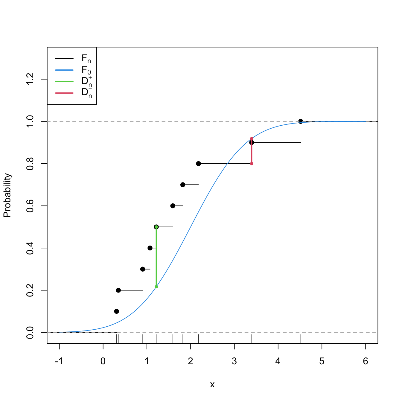

$Computation of the Kolmogorov–Smirnov statistic $D_n=\max(D_n^+,D_n^-)$ for a sample of size $n=10$ coming from $F_0(\cdot)=\Phi\left(\frac{\cdot-\mu_0}{\sigma_0}\right),$ where $\mu_0=2$ and $\sigma_0=1.$ In the example shown, $D_n=D_n^+.$$

Figure 6.1: Computation of the Kolmogorov–Smirnov statistic $D_n=\max(D_n^+,D_n^-)$ for a sample of size $n=10$ coming from $F_0(\cdot)=\Phi\left(\frac{\cdot-\mu_0}{\sigma_0}\right),$ where $\mu_0=2$ and $\sigma_0=1.$ In the example shown, $D_n=D_n^+.$

Exercise 6.1 Modify the parameters mu0 and sd0 in the previous code in order to have $F\neq F_0.$ What happens with $\sup_{x\in\mathbb{R}} \left|F_n(x)-F_0(x)\right|$?

Let’s see an example of the use of ks.test (also available as stats::ks.test), the function in base R.

# Sample data from a N(0, 1)
n <- 50
set.seed(3245678)
x <- rnorm(n = n)

# Kolmogorov-Smirnov test for H_0: F = N(0, 1). Does not reject
(ks <- ks.test(x = x, y = "pnorm")) # In "y" we specify F0 as a function
## 
##  Exact one-sample Kolmogorov-Smirnov test
## 
## data:  x
## D = 0.050298, p-value = 0.9989
## alternative hypothesis: two-sided

# Structure of "htest" class
str(ks)
## List of 7
##  $ statistic  : Named num 0.0503
##   ..- attr(*, "names")= chr "D"
##  $ p.value    : num 0.999
##  $ alternative: chr "two-sided"
##  $ method     : chr "Exact one-sample Kolmogorov-Smirnov test"
##  $ data.name  : chr "x"
##  $ data       :List of 2
##   ..$ x: num [1:50] 0.01911 0.0099 -0.01005 -0.02856 0.00282 ...
##   ..$ y:function (q, mean = 0, sd = 1, lower.tail = TRUE, log.p = FALSE)  
##  $ exact      : logi TRUE
##  - attr(*, "class")= chr [1:2] "ks.test" "htest"

# Kolmogorov-Smirnov test for H_0: F = N(0.5, 1). Rejects
ks.test(x = x, y = "pnorm", mean = 0.5)
## 
##  Exact one-sample Kolmogorov-Smirnov test
## 
## data:  x
## D = 0.24708, p-value = 0.003565
## alternative hypothesis: two-sided

# Kolmogorov-Smirnov test for H_0: F = Exp(2). Strongly rejects
ks.test(x = x, y = "pexp", rate = 1/2)
## 
##  Exact one-sample Kolmogorov-Smirnov test
## 
## data:  x
## D = 0.53495, p-value = 6.85e-14
## alternative hypothesis: two-sided

The following chunk of code shows how to call dgof::ks.test to perform a correct Kolmogorov–Smirnov when $F_0$ is discrete.

# Sample data from a Pois(5)
n <- 100
set.seed(3245678)
x <- rpois(n = n, lambda = 5)

# Kolmogorov-Smirnov test for H_0: F = Pois(5) without specifying that the
# distribution is discrete. Rejects (!?) giving a warning message
ks.test(x = x, y = "ppois", lambda = 5)
## 
##  Asymptotic one-sample Kolmogorov-Smirnov test
## 
## data:  x
## D = 0.20596, p-value = 0.0004135
## alternative hypothesis: two-sided

# We rely on dgof::ks.test, which works as stats::ks.test if the "y" argument
# is not marked as a "stepfun" object, the way the dgof package codifies
# discrete distribution functions

# Step function containing the cdf of the Pois(5). The "x" stands for the
# location of the steps and "y" for the value of the steps. "y" needs to have
# an extra point for the initial value of the function before the first step
x_eval <- 0:20
ppois_stepfun <- stepfun(x = x_eval, y = c(0, ppois(q = x_eval, lambda = 5)))
plot(ppois_stepfun, main = "Cdf of a Pois(5)")


# Kolmogorov-Smirnov test for H_0: F = Pois(5) adapted for discrete data,
# with data coming from a Pois(5)
dgof::ks.test(x = x, y = ppois_stepfun)
## 
##  One-sample Kolmogorov-Smirnov test
## 
## data:  x
## D = 0.032183, p-value = 0.9999
## alternative hypothesis: two-sided

# If data is normally distributed, the test rejects H_0
dgof::ks.test(x = rnorm(n = n, mean = 5), y = ppois_stepfun)
## 
##  One-sample Kolmogorov-Smirnov test
## 
## data:  rnorm(n = n, mean = 5)
## D = 0.38049, p-value = 5.321e-13
## alternative hypothesis: two-sided

Exercise 6.2 Implement the Kolmogorov–Smirnov test by:

Coding a function to compute the test statistic (6.2) from a sample $X_1,\ldots,X_n$ and a cdf $F_0.$
Implementing the $K$ function (6.3).
Calling the previous functions from a routine that returns the asymptotic $p$-value of the test.

Check that the implementations coincide with the ones of the ks.test function when exact = FALSE for data simulated from a $\mathcal{U}(0,1)$ and any $n.$ Note: ks.test computes $D_n/\sqrt{n}$ instead of $D_n.$

The following code chunk exemplifies with a small simulation study how the distribution of the $p$-values²¹⁶ is uniform if $H_0$ holds, and how it becomes more concentrated about $0$ when $H_1$ holds.

# Simulation of p-values when H_0 is true
set.seed(131231)
n <- 100
M <- 1e4
pvalues_H0 <- sapply(1:M, function(i) {
  x <- rnorm(n) # N(0, 1)
  ks.test(x, "pnorm")$p.value
})

# Simulation of p-values when H_0 is false -- the data does not
# come from a N(0, 1) but from a N(0, 2)
pvalues_H1 <- sapply(1:M, function(i) {
  x <- rnorm(n, mean = 0, sd = sqrt(2)) # N(0, 2)
  ks.test(x, "pnorm")$p.value
})

# Comparison of p-values
par(mfrow = 1:2)
hist(pvalues_H0, breaks = seq(0, 1, l = 20), probability = TRUE,
     main = latex2exp::TeX("$H_0$"), ylim = c(0, 10))
abline(h = 1, col = 2)
hist(pvalues_H1, breaks = seq(0, 1, l = 20), probability = TRUE,
     main = latex2exp::TeX("$H_1$"), ylim = c(0, 10))
abline(h = 1, col = 2)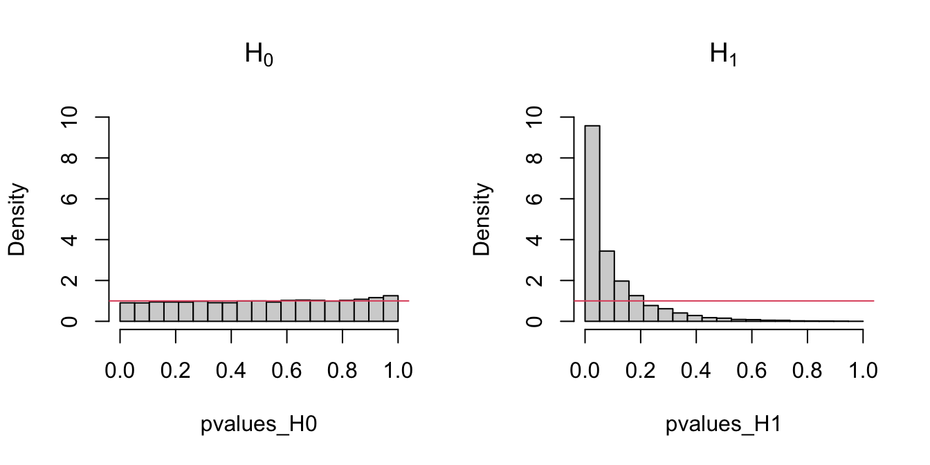

$Comparison of the distribution of $p$-values under $H_0$ and $H_1$ for the Kolmogorov–Smirnov test. Observe that the frequency of low $p$-values, associated with the rejection of $H_0,$ increases when $H_0$ does not hold. Under $H_0,$ the distribution of the $p$-values is uniform.$

Figure 6.2: Comparison of the distribution of $p$-values under $H_0$ and $H_1$ for the Kolmogorov–Smirnov test. Observe that the frequency of low $p$-values, associated with the rejection of $H_0,$ increases when $H_0$ does not hold. Under $H_0,$ the distribution of the $p$-values is uniform.

Exercise 6.3 Modify the parameters of the normal distribution used to sample under $H_1$ in order to increase and decrease the deviation from $H_0.$ What do you observe in the resulting distributions of the $p$-values?

6.1.1.2 Cramér–von Mises test

Test purpose. Given $X_1,\ldots,X_n\sim F,$ it tests $H_0: F=F_0$ vs. $H_1: F\neq F_0$ consistently against all the alternatives in $H_1.$
Statistic definition. The test statistic uses a quadratic distance²¹⁷ between $F_n$ and $F_0$:

\[\begin{align} W_n^2:=n\int(F_n(x)-F_0(x))^2\,\mathrm{d}F_0(x).\tag{6.4} \end{align}\]

If $H_0: F=F_0$ holds, then $W_n^2$ tends to be small. Hence, rejection happens for large values of $W_n^2.$
Statistic computation. The computation of $W_n^2$ can be significantly simplified by expanding the square in the integrand of (6.4) and then applying the change of variables $u=F_0(x)$:

\[\begin{align} W_n^2=\sum_{i=1}^n\left\{U_{(i)}-\frac{2i-1}{2n}\right\}^2+\frac{1}{12n},\tag{6.5} \end{align}\]

where again $U_{(j)}$ stands for the $j$-th sorted $U_i=F_0(X_i),$ $i=1,\ldots,n.$
Distribution under $H_0.$ If $H_0$ holds and $F_0$ is continuous, then $W_n^2$ has an asymptotic cdf given by²¹⁸

\[\begin{align} \lim_{n\to\infty}\mathbb{P}[W_n^2\leq x]=&\,1-\frac{1}{\pi}\sum_{j=1}^\infty (-1)^{j-1}W_j(x),\tag{6.6}\\ W_j(x):=&\,\int_{(2j-1)^2\pi^2}^{4j^2\pi^2}\sqrt{\frac{-\sqrt{y}}{\sin\sqrt{y}}}\frac{e^{-\frac{xy}{2}}}{y}\,\mathrm{d}y.\nonumber \end{align}\]
Highlights and caveats. By a reasoning analogous to the one done in the Kolmogorov–Smirnov test, the Cramér–von Mises test can be seen to be distribution-free if $F_0$ is continuous and the sample has no ties. Otherwise, (6.6) is not the true asymptotic distribution. Although the Kolmogorov–Smirnov test is the most popular ecdf-based test, empirical evidence suggests that the Cramér–von Mises test is often more powerful than the Kolmogorov–Smirnov test for a broad class of alternative hypotheses.²¹⁹
Implementation in R. For continuous data, the test statistic $W_n^2$ and the asymptotic $p$-value are implemented in the goftest::cvm.test function. The asymptotic cdf (6.6) is given in goftest::pCvM (goftest::qCvM computes its inverse). For discrete $F_0,$ see dgof::cvm.test.

The following chunk of code points to the implementation of the Cramér–von Mises test.

# Sample data from a N(0, 1)
set.seed(3245678)
n <- 50
x <- rnorm(n = n)

# Cramér-von Mises test for H_0: F = N(0, 1). Does not reject
goftest::cvm.test(x = x, null = "pnorm")
## 
##  Cramer-von Mises test of goodness-of-fit
##  Null hypothesis: Normal distribution
##  Parameters assumed to be fixed
## 
## data:  x
## omega2 = 0.022294, p-value = 0.9948

# Comparison with Kolmogorov-Smirnov
ks.test(x = x, y = "pnorm")
## 
##  Exact one-sample Kolmogorov-Smirnov test
## 
## data:  x
## D = 0.050298, p-value = 0.9989
## alternative hypothesis: two-sided

# Sample data from a Pois(5)
set.seed(3245678)
n <- 100
x <- rpois(n = n, lambda = 5)

# Cramér-von Mises test for H_0: F = Pois(5) without specifying that the
# distribution is discrete. Rejects (!?) without giving a warning message
goftest::cvm.test(x = x, null = "ppois", lambda = 5)
## 
##  Cramer-von Mises test of goodness-of-fit
##  Null hypothesis: Poisson distribution
##  with parameter lambda = 5
##  Parameters assumed to be fixed
## 
## data:  x
## omega2 = 0.74735, p-value = 0.009631

# We rely on dgof::cvm.test and run a Cramér-von Mises test for H_0: F = Pois(5)
# adapted for discrete data, with data coming from a Pois(5)
x_eval <- 0:20
ppois_stepfun <- stepfun(x = x_eval, y = c(0, ppois(q = x_eval, lambda = 5)))
dgof::cvm.test(x = x, y = ppois_stepfun)
## 
##  Cramer-von Mises - W2
## 
## data:  x
## W2 = 0.038256, p-value = 0.9082
## alternative hypothesis: Two.sided

# Plot the asymptotic null distribution function
curve(goftest::pCvM(x), from = 0, to = 1, n = 300)

Exercise 6.4 Implement the Cramér–von Mises test by:

Coding the Cramér–von Mises statistic (6.5) from a sample $X_1,\ldots,X_n$ and a cdf $F_0.$ Check that the implementation coincides with the one of the goftest::cvm.test function.
Computing the asymptotic $p$-value using goftest::pCvM. Compare this asymptotic $p$-value with the exact $p$-value given by goftest::cvm.test, observing that for a large $n$ the difference is inappreciable.

Exercise 6.5 Verify the correctness of the asymptotic null distribution of $W_n^2$ that was given in (6.6). To do so, numerically implement $W_j(x)$ and compute (6.6). Validate your implementation by:

Simulating $M=1,000$ samples of size $n=200$ under $H_0,$ obtaining $M$ statistics $W_{n;1}^{2},\ldots, W_{n;M}^{2},$ and plotting their ecdf.
Overlaying your asymptotic cdf and the one provided by goftest::pCvM.
Checking that the three curves approximately coincide.

6.1.1.3 Anderson–Darling test

Test purpose. Given $X_1,\ldots,X_n\sim F,$ it tests $H_0: F=F_0$ vs. $H_1: F\neq F_0$ consistently against all the alternatives in $H_1.$
Statistic definition. The test statistic uses a quadratic distance between $F_n$ and $F_0$ weighted by $w(x)=(F_0(x)(1-F_0(x)))^{-1}$:

\[\begin{align*} A_n^2:=n\int\frac{(F_n(x)-F_0(x))^2}{F_0(x)(1-F_0(x))}\,\mathrm{d}F_0(x). \end{align*}\]

If $H_0$ holds, then $A_n^2$ tends to be small (because of the denominator). Hence, rejection happens for large values of $A_n^2.$ Note that, compared with $W_n^2,$ $A_n^2$ places more weight on the deviations between $F_n(x)$ and $F_0(x)$ that happen on the tails, that is, when $F_0(x)\approx 0$ or $F_0(x)\approx 1.$²²⁰ $\!\!^,$²²¹
Statistic computation. The computation of $A_n^2$ can be significantly simplified:

\[\begin{align} A_n^2=-n-\frac{1}{n}\sum_{i=1}^n&\Big\{(2i-1)\log(U_{(i)})\nonumber\\ &+(2n+1-2i)\log(1-U_{(i)})\Big\}.\tag{6.7} \end{align}\]
Distribution under $H_0.$ If $H_0$ holds and $F_0$ is continuous, then the asymptotic cdf of $A_n^2$ is the cdf of the random variable

\[\begin{align} \sum_{j=1}^\infty\frac{Y_j}{j(j+1)},\quad \text{where } Y_j\sim\chi^2_1,\,j\geq 1,\text{ are iid}.\tag{6.8} \end{align}\]

Unfortunately, the cdf of (6.8) does not admit a simple analytical expression. It can, however, be approximated by Monte Carlo by sampling from the random variable (6.8).
Highlights and caveats. As with the previous tests, the Anderson–Darling test is also distribution-free if $F_0$ is continuous and there are no ties in the sample. Otherwise, the null asymptotic distribution is different from the one of (6.8). As for the Cramér–von Mises test, there is also empirical evidence indicating that the Anderson–Darling test is more powerful than the Kolmogorov–Smirnov test for a broad class of alternative hypotheses. In addition, due to its construction, the Anderson–Darling test is able to detect better the situations in which $F_0$ and $F$ differ on the tails (that is, for extreme data).
Implementation in R. For continuous data, the test statistic $A_n^2$ and the asymptotic $p$-value are implemented in the goftest::ad.test function. The asymptotic cdf of (6.8) is given in goftest::pAD (goftest::qAD computes its inverse). For discrete $F_0,$ see dgof::cvm.test with type = "A2".

The following code chunk illustrates the implementation of the Anderson–Darling test.

# Sample data from a N(0, 1)
set.seed(3245678)
n <- 50
x <- rnorm(n = n)

# Anderson-Darling test for H_0: F = N(0, 1). Does not reject
goftest::ad.test(x = x, null = "pnorm")
## 
##  Anderson-Darling test of goodness-of-fit
##  Null hypothesis: Normal distribution
##  Parameters assumed to be fixed
## 
## data:  x
## An = 0.18502, p-value = 0.994

# Sample data from a Pois(5)
set.seed(3245678)
n <- 100
x <- rpois(n = n, lambda = 5)

# Anderson-Darling test for H_0: F = Pois(5) without specifying that the
# distribution is discrete. Rejects (!?) without giving a warning message
goftest::ad.test(x = x, null = "ppois", lambda = 5)
## 
##  Anderson-Darling test of goodness-of-fit
##  Null hypothesis: Poisson distribution
##  with parameter lambda = 5
##  Parameters assumed to be fixed
## 
## data:  x
## An = 3.7279, p-value = 0.01191

# We rely on dgof::cvm.test and run an Anderson-Darling test for H_0: F = Pois(5)
# adapted for discrete data, with data coming from a Pois(5)
x_eval <- 0:20
ppois_stepfun <- stepfun(x = x_eval, y = c(0, ppois(q = x_eval, lambda = 5)))
dgof::cvm.test(x = x, y = ppois_stepfun, type = "A2")
## 
##  Cramer-von Mises - A2
## 
## data:  x
## A2 = 0.3128, p-value = 0.9057
## alternative hypothesis: Two.sided

# Plot the asymptotic null distribution function
curve(goftest::pAD(x), from = 0, to = 5, n = 300)

Exercise 6.6 Implement the Anderson–Darling test by:

Coding the Anderson–Darling statistic (6.7) from a sample $X_1,\ldots,X_n$ and a cdf $F_0.$ Check that the implementation coincides with the one of the goftest::ad.test function.
Computing the asymptotic $p$-value using goftest::pAD. Compare this asymptotic $p$-value with the exact $p$-value given by goftest::ad.test, observing that for large $n$ the difference is inappreciable.

Exercise 6.7 Verify the correctness of the asymptotic representation of $A_n^2$ that was given in (6.8). To do so:

Simulate $M=1,000$ samples of size $n=200$ under $H_0,$ obtain $M$ statistics $A_{n;1}^{2},\ldots, A_{n;M}^{2},$ and draw its histogram.
Simulate $M$ samples from the random variable (6.8) and draw its histogram.
Check that the two histograms approximately coincide.

Exercise 6.8 Let’s investigate empirically the performance of the Kolmogorov–Smirnov, Cramér–von Mises, and Anderson–Darling tests for a specific scenario. We consider $H_0:X\sim \mathcal{N}(0,1)$ and the following simulation study:

Generate $M=1,000$ samples of size $n$ from $\mathcal{N}(\mu,1).$
For each sample, test $H_0$ with the three tests.
Obtain the relative frequency of rejections at level $\alpha$ for each test.
Draw three histograms for the $p$-values in the spirit of Figure 6.3.

In order to cleanly perform the previous steps for several choices of $(n,\mu,\alpha),$ code a function that performs the simulation study from those arguments and gives something similar to Figure 6.3 as output. Then, use the following settings and accurately comment on the outcome of each of them:

$H_0$ holds.
- Take $n=25,$ $\mu=0,$ and $\alpha=0.05.$ Check that the relative frequency of rejections is about $\alpha.$
- Take $n=25,$ $\mu=0,$ and $\alpha=0.10.$
- Take $n=100,$ $\mu=0,$ and $\alpha=0.10.$
$H_0$ does not hold.
- $n=25,$ $\mu=0.25,$ $\alpha=0.05.$ Check that the relative frequency of rejections is above $\alpha.$
- $n=50,$ $\mu=0.25,$ $\alpha=0.05.$
- $n=25,$ $\mu=0.50,$ $\alpha=0.05.$
- Replace $\mathcal{N}(\mu,1)$ with $t_{10}.$ Take $n=50$ and $\alpha=0.05.$ Which test is clearly better? Why?

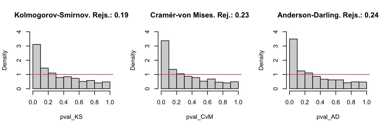
$The histograms of the $p$-values and the relative rejection frequencies for the Kolmogorov–Smirnov, Cramér–von Mises, and Anderson–Darling tests. The null hypothesis is $H_0:X\sim \mathcal{N}(0,1)$ and the sample of size $n=25$ is generated from a $\mathcal{N}(0.25,1).$ The significance level is $\alpha=0.05$.$

Figure 6.3: The histograms of the $p$-values and the relative rejection frequencies for the Kolmogorov–Smirnov, Cramér–von Mises, and Anderson–Darling tests. The null hypothesis is $H_0:X\sim \mathcal{N}(0,1)$ and the sample of size $n=25$ is generated from a $\mathcal{N}(0.25,1).$ The significance level is $\alpha=0.05$.

6.1.2 Normality tests

The tests seen in the previous section have a very notable practical limitation: they require complete knowledge of $F_0,$ the hypothesized distribution for $X.$ In practice, such a precise knowledge about $X$ is unrealistic. Practitioners are more interested in answering more general questions, one of them being:

Is the data “normally distributed”?

With the statement “$X$ is normally distributed” we refer to the fact that $X\sim \mathcal{N}(\mu,\sigma^2)$ for certain parameters $\mu\in\mathbb{R}$ and $\sigma\in\mathbb{R^+},$ possibly unknown. This statement is notably more general than “$X$ is distributed as a $\mathcal{N}(0,1)$” or “$X$ is distributed as a $\mathcal{N}(0.1,1.3)$”.

The test for normality is formalized as follows. Given an iid sample $X_1,\ldots,X_n$ from the distribution $F,$ we test the null hypothesis

\[\begin{align} H_0:F\in\mathcal{F}_{\mathcal{N}}:=\left\{\Phi\left(\frac{\cdot-\mu}{\sigma}\right):\mu\in\mathbb{R},\sigma\in\mathbb{R}^+\right\},\tag{6.9} \end{align}\]

where $\mathcal{F}_{\mathcal{N}}$ is the class of normal distributions, against the most general alternative

\[\begin{align*} H_1:F\not\in\mathcal{F}_{\mathcal{N}}. \end{align*}\]

Comparing (6.9) with (6.1), it is evident that the former is more general, as a range of possible values for $F$ is included in $H_0.$ This is the reason why $H_0$ is called a composite null hypothesis, rather than a simple null hypothesis, as (6.1) was.

The testing of (6.9) requires the estimation of the unknown parameters $(\mu,\sigma).$ Their maximum likelihood estimators are $(\bar{X},S),$ where $S:=\sqrt{\frac{1}{n}\sum_{i=1}^n(X_i-\bar{X})^2}$ is the sample standard deviation. Therefore, a tempting possibility is to apply the tests seen in Section 6.1.1 to

\[\begin{align*} H_0:F=\Phi\left(\frac{\cdot-\bar{X}}{S}\right). \end{align*}\]

However, as warned at the beginning of Section 6.1, this naive approach would result in seriously conservative tests that would fail to reject $H_0$ adequately. The intuitive explanation is simple: when estimating $(\mu,\sigma)$ from the sample we are obtaining the closest normal cdf to $F,$ that is, $\Phi\left(\frac{\cdot-\bar{X}}{S}\right).$ Therefore, setting $F_0=\Phi\left(\frac{\cdot-\bar{X}}{S}\right)$ and then running one of the ecdf-based tests on $H_0:F=F_0$ will ignore this estimation step, which will bias the test decision towards $H_0$.

Adequately accounting for the estimation of $(\mu,\sigma)$ amounts to study the asymptotic distributions under $H_0$ of the test statistics that are computed with the data-dependent cdf $\Phi\left(\frac{\cdot-\bar{X}}{S}\right)$ in the place of $F_0.$ This is what is precisely done by the tests that adapt the ecdf-based tests seen in Section 6.1.1 by

replacing $F_0$ with $\Phi\left(\frac{\cdot-\bar{X}}{S}\right)$ in the formulation of the test statistics;
replacing $U_i$ with $P_i:=\Phi\left(\frac{X_i-\bar{X}}{\hat{S}}\right),$ $i=1,\ldots,n,$ in the computational forms of the statistics;²²²
obtaining a different null asymptotic distribution that is usually more convoluted and is approximated by tabulation or simulation.

6.1.2.1 Lilliefors test (Kolmogorov–Smirnov test for normality)

Test purpose. Given $X_1,\ldots,X_n,$ it tests $H_0: F\in\mathcal{F}_\mathcal{N}$ vs. $H_1: F\not\in\mathcal{F}_\mathcal{N}$ consistently against all the alternatives in $H_1.$
Statistic definition and computation. The test statistic uses the supremum distance between $F_n$ and $\Phi\left(\frac{\cdot-\bar{X}}{S}\right)$:

\[\begin{align*} D_n=&\,\sqrt{n}\sup_{x\in\mathbb{R}} \left|F_n(x)-\Phi\left(\frac{x-\bar{X}}{S}\right)\right|=\max(D_n^+,D_n^-),\\ D_n^+=&\,\sqrt{n}\max_{1\leq i\leq n}\left\{\frac{i}{n}-P_{(i)}\right\},\\ D_n^-=&\,\sqrt{n}\max_{1\leq i\leq n}\left\{P_{(i)}-\frac{i-1}{n}\right\}, \end{align*}\]

where $P_{(j)}$ stands for the $j$-th sorted $P_i=\Phi\left(\frac{X_i-\bar{X}}{S}\right),$ $i=1,\ldots,n.$ Clearly, if $H_0$ holds, then $D_n$ tends to be small. Hence, rejection happens when $D_n$ is large.
Distribution under $H_0.$ If $H_0$ holds, the critical values at level of significance $\alpha$ can be obtained from Lilliefors (1967).²²³ Dallal and Wilkinson (1986) provides an analytical approximation to the null distribution.
Highlights and caveats. The Lilliefors test is not distribution-free, in the sense that the null distribution of the test statistic clearly depends on the normality assumption. However, it is parameter-free, since the distribution does not depend on the actual parameters $(\mu,\sigma)$ for which $F=\Phi\left(\frac{\cdot-\mu}{\sigma}\right)$ is satisfied. This result comes from the iid sample $X_1,\ldots,X_n\stackrel{H_0}{\sim} \mathcal{N}(\mu,\sigma^2)$ generating the id sample $\frac{X_1-\bar{X}}{S},\ldots,\frac{X_n-\bar{X}}{S}\stackrel{H_0}{\sim} \tilde{f}_0,$ where $\tilde{f}_0$ is a certain pdf that does not depend on $(\mu,\sigma).$²²⁴ Therefore, $P_1,\ldots,P_n$ is an id sample that does not depend on $(\mu,\sigma).$
Implementation in R. The nortest::lillie.test function implements the test.

6.1.2.2 Cramér–von Mises normality test

Test purpose. Given $X_1,\ldots,X_n,$ it tests $H_0: F\in\mathcal{F}_\mathcal{N}$ vs. $H_1: F\not\in\mathcal{F}_\mathcal{N}$ consistently against all the alternatives in $H_1.$
Statistic definition and computation. The test statistic uses the quadratic distance between $F_n$ and $\Phi\left(\frac{\cdot-\bar{X}}{S}\right)$:

\[\begin{align*} W_n^2=&\,n\int\left(F_n(x)-\Phi\left(\frac{x-\bar{X}}{S}\right)\right)^2\,\mathrm{d}\Phi\left(\frac{x-\bar{X}}{S}\right)\\ =&\,\sum_{i=1}^n\left\{P_{(i)}-\frac{2i-1}{2n}\right\}^2+\frac{1}{12n}, \end{align*}\]

where $P_{(j)}$ stands for the $j$-th sorted $P_i=\Phi\left(\frac{X_i-\bar{X}}{S}\right),$ $i=1,\ldots,n.$ Rejection happens when $W_n^2$ is large.
Distribution under $H_0.$ If $H_0$ holds, the $p$-values of the test can be approximated using Table 4.9 in D’Agostino and Stephens (1986).
Highlights and caveats. Like the Lilliefors test, the Cramér–von Mises test is also parameter-free. Its usual power superiority over the Kolmogorov–Smirnov also extends to the testing of normality.
Implementation in R. The nortest::cvm.test function implements the test.

6.1.2.3 Anderson–Darling normality test

Test purpose. Given $X_1,\ldots,X_n,$ it tests $H_0: F\in\mathcal{F}_\mathcal{N}$ vs. $H_1: F\not\in\mathcal{F}_\mathcal{N}$ consistently against all the alternatives in $H_1.$
Statistic definition and computation. The test statistic uses a weighted quadratic distance between $F_n$ and $\Phi\left(\frac{\cdot-\bar{X}}{S}\right)$:

\[\begin{align*} A_n^2=&\,n\int\frac{\left(F_n(x)-\Phi\left(\frac{x-\bar{X}}{S}\right)\right)^2}{\Phi\left(\frac{x-\bar{X}}{S}\right)\left(1-\Phi\left(\frac{x-\bar{X}}{S}\right)\right)}\,\mathrm{d}\Phi\left(\frac{x-\bar{X}}{S}\right)\\ =&\,-n-\frac{1}{n}\sum_{i=1}^n\left\{(2i-1)\log(P_{(i)})+(2n+1-2i)\log(1-P_{(i)})\right\}. \end{align*}\]

Rejection happens when $A_n^2$ is large.
Distribution under $H_0.$ If $H_0$ holds, the $p$-values of the test can be approximated using Table 4.9 in D’Agostino and Stephens (1986).
Highlights and caveats. The test is also parameter-free. Since the test statistic places more weight on the tails than the Cramér–von Mises, it is better suited for detecting heavy-tailed deviations from normality.
Implementation in R. The nortest::ad.test function implements the test.

The following code chunk gives the implementation of these normality tests.

# Sample data from a N(10, 1)
set.seed(981589472)
n <- 200
x <- rnorm(n = n, mean = 10)

# Normality tests -- do not reject H0
nortest::lillie.test(x = x)
## 
##  Lilliefors (Kolmogorov-Smirnov) normality test
## 
## data:  x
## D = 0.037754, p-value = 0.6951
nortest::cvm.test(x = x)
## 
##  Cramer-von Mises normality test
## 
## data:  x
## W = 0.052993, p-value = 0.4662
nortest::ad.test(x = x)
## 
##  Anderson-Darling normality test
## 
## data:  x
## A = 0.38898, p-value = 0.3816

# Sample data from a Student's t with 3 degrees of freedom
x <- rt(n = n, df = 3)

# Normality tests -- reject H0
nortest::lillie.test(x = x)
## 
##  Lilliefors (Kolmogorov-Smirnov) normality test
## 
## data:  x
## D = 0.06958, p-value = 0.01979
nortest::cvm.test(x = x)
## 
##  Cramer-von Mises normality test
## 
## data:  x
## W = 0.24584, p-value = 0.001432
nortest::ad.test(x = x)
## 
##  Anderson-Darling normality test
## 
## data:  x
## A = 1.5929, p-value = 0.000415

# Flawed normality tests -- do not reject because the null distribution
# that is employed is wrong!
ks.test(x = x, y = "pnorm", mean = mean(x), sd = sd(x))
## 
##  Asymptotic one-sample Kolmogorov-Smirnov test
## 
## data:  x
## D = 0.06958, p-value = 0.2876
## alternative hypothesis: two-sided
goftest::cvm.test(x = x, null = "pnorm", mean = mean(x), sd = sd(x))
## 
##  Cramer-von Mises test of goodness-of-fit
##  Null hypothesis: Normal distribution
##  with parameters mean = 0.0238254313803778, sd = 1.6388504082364
##  Parameters assumed to be fixed
## 
## data:  x
## omega2 = 0.24584, p-value = 0.1938
goftest::ad.test(x = x, null = "pnorm", mean = mean(x), sd = sd(x))
## 
##  Anderson-Darling test of goodness-of-fit
##  Null hypothesis: Normal distribution
##  with parameters mean = 0.0238254313803778, sd = 1.6388504082364
##  Parameters assumed to be fixed
## 
## data:  x
## An = 1.5929, p-value = 0.1558

6.1.2.4 Shapiro–Francia normality test

We now consider a different normality test that is not based on the ecdf, the Shapiro–Francia normality test. This test is a modification of the wildly popular Shapiro–Wilk test, but the Shapiro–Francia test is easier to interpret and explain.²²⁵

The test is based on the QQ-plot of the sample $X_1,\ldots,X_n.$ The plot is composed of the pairs $\left(\Phi^{-1}\left(\frac{i}{n+1}\right),X_{(i)}\right)\,,$ for $i=1,\ldots,n.$²²⁶ That is, the QQ-plot plots $\mathcal{N}(0,1)$-quantiles against sample quantiles.

Since the $\alpha$-lower quantile of a $\mathcal{N}(\mu,\sigma^2),$ $z_{\alpha;\mu,\sigma},$ verifies that

\[\begin{align} z_{\alpha;\mu,\sigma}=\mu+\sigma z_{\alpha;0,1},\tag{6.10} \end{align}\]

then, if the sample is distributed as a $\mathcal{N}(\mu,\sigma^2),$ the points of the QQ-plot are expected to align about the straight line (6.10). This is illustrated in the code below.

n <- 100
mu <- 10
sigma <- 2
set.seed(12345678)
x <- rnorm(n, mean = mu, sd = sigma)
qqnorm(x)
abline(a = mu, b = sigma, col = 2)

$QQ-plot (qqnorm) for data simulated from a $\mathcal{N}(\mu,\sigma^2)$ and theoretical line $y=\mu+\sigma x$ (red).$

Figure 6.4: QQ-plot (qqnorm) for data simulated from a $\mathcal{N}(\mu,\sigma^2)$ and theoretical line $y=\mu+\sigma x$ (red).

The QQ-plot can therefore be used as a graphical check for normality: if the data is distributed about some straight line, then it likely is normally distributed. However, this graphical check is subjective and, to complicate things further, it is usual for departures from the diagonal to be larger in the extremes than in the center, even under normality, although these departures are more evident if the data is non-normal.²²⁷ Figure 6.5, generated with the code below, depicts the uncertainty behind the QQ-plot.

M <- 1e3
n <- 100
plot(0, 0, xlim = c(-3.5, 3.5), ylim = c(-3.5, 3.5), type = "n",
     xlab = "Theoretical Quantiles", ylab = "Sample Quantiles",
     main = "Confidence bands for QQ-plot")
x <- matrix(rnorm(M * n), nrow = n, ncol = M)
matpoints(qnorm(ppoints(n)), apply(x, 2, sort), pch = 19, cex = 0.5,
          col = gray(0, alpha = 0.01))
abline(a = 0, b = 1)
p <- seq(0, 1, l = 1e4)
xi <- qnorm(p)
lines(xi, xi - qnorm(0.975) / sqrt(n) * sqrt(p * (1 - p)) / dnorm(xi),
      col = 2, lwd = 2)
lines(xi, xi + qnorm(0.975) / sqrt(n) * sqrt(p * (1 - p)) / dnorm(xi),
      col = 2, lwd = 2)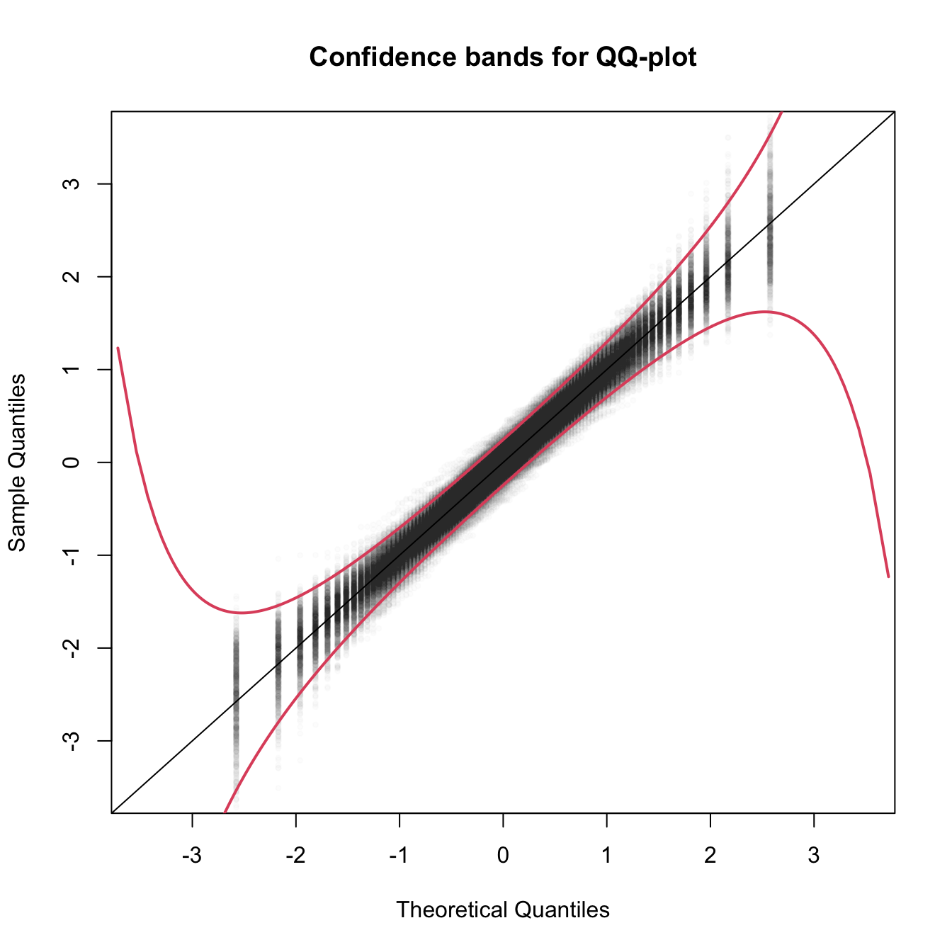

$The uncertainty behind the QQ-plot. The figure aggregates $M=1,000$ different QQ-plots of $\mathcal{N}(0,1)$ data with $n=100,$ displaying for each of them the pairs $(x_p,\hat x_p)$ evaluated at $p=\frac{i-1/2}{n},$ $i=1,\ldots,n$ (as they result from ppoints(n)). The uncertainty is measured by the asymptotic $100(1-\alpha)\%$ CIs for $\hat x_p,$ given by $\left(x_p\pm\frac{z_{\alpha/2}}{\sqrt{n}}\frac{\sqrt{p(1-p)}}{\phi(x_p)}\right).$ These curves are displayed in red for $\alpha=0.05.$ Observe that the vertical strips arise because the $x_p$ coordinate is deterministic.$

Figure 6.5: The uncertainty behind the QQ-plot. The figure aggregates $M=1,000$ different QQ-plots of $\mathcal{N}(0,1)$ data with $n=100,$ displaying for each of them the pairs $(x_p,\hat x_p)$ evaluated at $p=\frac{i-1/2}{n},$ $i=1,\ldots,n$ (as they result from ppoints(n)). The uncertainty is measured by the asymptotic $100(1-\alpha)\%$ CIs for $\hat x_p,$ given by $\left(x_p\pm\frac{z_{\alpha/2}}{\sqrt{n}}\frac{\sqrt{p(1-p)}}{\phi(x_p)}\right).$ These curves are displayed in red for $\alpha=0.05.$ Observe that the vertical strips arise because the $x_p$ coordinate is deterministic.

The Shapiro–Francia test evaluates how tightly distributed the QQ plot is about the linear trend that must arise if the data is normally distributed.

Test purpose. Given $X_1,\ldots,X_n,$ it tests $H_0: F\in\mathcal{F}_\mathcal{N}$ vs. $H_1: F\not\in\mathcal{F}_\mathcal{N}$ consistently against all the alternatives in $H_1.$
Statistic definition and computation. The test statistic, $W_n',$ is simply the squared correlation coefficient for the sample²²⁸

\[\begin{align*} \left(\Phi^{-1}\left(\frac{i - 3/8}{n-1/4}\right),X_{(i)}\right),\quad i=1,\ldots,n. \end{align*}\]
Distribution under $H_0.$ Royston (1993) derived a simple analytical formula that serves to approximate the null distribution of $W_n'$ for $5\leq n\leq 5,000.$
Highlights and caveats. The test is also parameter-free, since its distribution does not depend on the actual parameters $(\mu,\sigma)$ for which the equality $H_0$ holds.
Implementation in R. The nortest::sf.test function implements the test. The condition $5\leq n\leq 5,000$ is enforced by the function.²²⁹

The use of the function is described below.

# Does not reject H0
set.seed(123456)
n <- 100
x <- rnorm(n = n, mean = 10)
nortest::sf.test(x)
## 
##  Shapiro-Francia normality test
## 
## data:  x
## W = 0.99336, p-value = 0.8401

# Rejects H0
x <- rt(n = n, df = 3)
nortest::sf.test(x)
## 
##  Shapiro-Francia normality test
## 
## data:  x
## W = 0.91545, p-value = 2.754e-05

# Test statistic
cor(x = sort(x), y = qnorm(ppoints(n, a = 3/8)))^2
## [1] 0.9154466

Exercise 6.9 The gamma distribution can be approximated by a normal distribution. Precisely, $\Gamma(\lambda,n)\approx\mathcal{N}\left(\frac{n}{\lambda},\frac{n}{\lambda^2}\right)$ when $n\to\infty.$ The following simulation study is designed to evaluate the accuracy of the approximation with $n\to\infty$ using goodness-of-fit tests. For that purpose, we generate $X_1,\ldots,X_m\sim\Gamma(\lambda,n)$ and run the following tests:

The Kolmogorov–Smirnov, Cramér–von Mises, and Anderson–Darling tests, where $F_0$ stands for the cdf of $\mathcal{N}\left(\frac{n}{\lambda},\frac{n}{\lambda^2}\right).$
The normality adaptations of the previous tests.

Do:

Code a function that simulates $X_1,\ldots,X_m\sim\Gamma(\lambda,n)$ and returns the $p$-values of the aforementioned tests. The function must take as input $\lambda,$ $n,$ and $m.$ Call this function simulation.
Call the simulation function $M=500$ times for $\lambda=1,$ $n=20,$ and $m=100,$ and represent in a $2\times 3$ plot the histograms of the $p$-values of the six tests. Comment on the output.
Repeat the experiment for: (i) $n=50,200$ with $m=100;$ and (ii) $m=50,200$ with $n=50.$ Explain the interpretations of the effects of $n$ and $m$ in the results.

6.1.3 Bootstrap-based approach to goodness-of-fit testing

Each normality test discussed in the previous section is an instance of a goodness-of-fit test for a parametric distribution model. Precisely, the normality tests are goodness-of-fit tests for the normal distribution model. Therefore, they address a specific instance of the test of the null composite hypothesis

\[\begin{align*} H_0:F\in\mathcal{F}_{\Theta}:=\left\{F_\theta:\theta\in\Theta\subset\mathbb{R}^q\right\}, \end{align*}\]

where $\mathcal{F}_{\Theta}$ denotes a certain parametric family of distributions indexed by the (possibly multidimensional) parameter $\theta\in\Theta,$ versus the most general alternative

\[\begin{align*} H_1:F\not\in\mathcal{F}_{\Theta}. \end{align*}\]

The normality case demonstrated that the goodness-of-fit tests for the simple hypothesis were not readily applicable, and that the null distributions were affected by the estimation of the unknown parameters $\theta=(\mu,\sigma).$ In addition, these null distributions tend to be cumbersome, requiring analytical approximations that have to be done on a test-by-test basis in order to obtain computable $p$-values.

To make things worse, the derivations that were done to obtain the asymptotic distributions of the normality test are not reusable if $\mathcal{F}_\Theta$ is different. For example, if we wanted to test exponentiality, that is,

\[\begin{align} H_0:F\in\mathcal{F}_{\mathbb{R}^+}=\left\{F_\theta(x)=(1-e^{-\theta x})1_{\{x>0\}}:\theta\in\mathbb{R}^+\right\},\tag{6.11} \end{align}\]

then new asymptotic distributions with their corresponding new analytical approximations would need to be derived. Clearly, this is not a very practical approach if we are to evaluate the goodness-of-fit of several parametric models. A practical computational-based solution is to rely on bootstrap, specifically, on parametric bootstrap.

Since the main problem is to establish the distribution of the test statistic under $H_0,$ then a possibility is to approximate this distribution by the distribution of the bootstrapped statistic. Precisely, let $T_n$ be the statistic computed from the sample

\[\begin{align*} X_1,\ldots,X_n\stackrel{H_0}{\sim}F_\theta \end{align*}\]

and let $T_n^*$ be its bootstrapped version, that is, the statistic computed from the simulated sample²³⁰

\[\begin{align} X^*_1,\ldots,X^*_n \sim F_{\hat\theta}.\tag{6.12} \end{align}\]

Then, if $H_0$ holds, the distribution of $T_n$ is approximated²³¹ by the one of $T_n^*$. In addition, since the sampling in (6.12) is completely under our control, we can approximate arbitrarily well the distribution of $T_n^*$ by Monte Carlo. For example, the computation of the upper tail probability $\mathbb{P}^*[T_n^*>x],$ required to obtain $p$-values in all the tests we have seen, can be done by

\[\begin{align*} \mathbb{P}^*[T_n^* > x]\approx\frac{1}{B}\sum_{b=1}^B 1_{\{T_n^{*b}> x\}}, \end{align*}\]

where $T_n^{*1},\ldots,T_n^{*B}$ is a sample from $T_n^*$ obtained by simulating $B$ bootstrap samples from (6.12).

The whole approach can be summarized in the following bootstrap-based procedure for performing a goodness-of-fit test for a parametric distribution model:

Estimate $\theta$ from the sample $X_1,\ldots,X_n,$ obtaining $\hat\theta$ (for example, use maximum likelihood).
Compute the statistic $T_n$ from $X_1,\ldots,X_n$ and $\hat\theta.$
Enter the “bootstrap world”. For $b=1,\ldots,B$:
1. Simulate a bootstrap sample $X_1^{*b},\ldots,X_n^{*b}$ from $F_{\hat\theta}.$
2. Compute $\hat\theta^{*b}$ from $X_1^{*b},\ldots,X_n^{*b}$ exactly in the same form that $\hat\theta$ was computed from $X_1,\ldots,X_n.$
3. Compute $T_n^{*b}$ from $X_1^{*b},\ldots,X_n^{*b}$ and $\hat\theta^{*b}.$
Obtain the $p$-value approximation

\[\begin{align*} p\text{-value}\approx\frac{1}{B}\sum_{b=1}^B 1_{\{T_n^{*b}> T_n\}} \end{align*}\]

and emit a test decision from it. Modify it accordingly if rejection of $H_0$ does not happen for large values of $T_n.$

The following chunk of code provides a template function for implementing the previous algorithm. The template is initialized with the specifics for testing (6.11), for which $\hat\theta_{\mathrm{ML}}=1/{\bar X}.$ The function uses the boot::boot function for carrying out the parametric bootstrap.

# A goodness-of-fit test of the exponential distribution using the
# Cramér-von Mises statistic
cvm_exp_gof <- function(x, B = 5e3, plot_boot = TRUE) {

  # Test statistic function (depends on the data only)
  Tn <- function(data) {

    # Maximum likelihood estimator -- MODIFY DEPENDING ON THE PROBLEM
    theta_hat <- 1 / mean(data)

    # Test statistic -- MODIFY DEPENDING ON THE PROBLEM
    goftest::cvm.test(x = data, null = "pexp", rate = theta_hat)$statistic

  }

  # Function to simulate bootstrap samples X_1^*, ..., X_n^*. Requires TWO
  # arguments, one being the data X_1, ..., X_n and the other containing
  # the parameter theta
  r_mod <- function(data, theta) {

    # Simulate from an exponential. In this case, the function only uses
    # the sample size from the data argument to estimate theta -- MODIFY
    # DEPENDING ON THE PROBLEM
    rexp(n = length(data), rate = 1 / theta)

  }

  # Estimate of theta -- MODIFY DEPENDING ON THE PROBLEM
  theta_hat <- 1 / mean(x)

  # Perform bootstrap resampling with the aid of boot::boot
  Tn_star <- boot::boot(data = x, statistic = Tn, sim = "parametric",
                        ran.gen = r_mod, mle = theta_hat, R = B)

  # Test information -- MODIFY DEPENDING ON THE PROBLEM
  method <- "Bootstrap-based Cramér-von Mises test for exponentiality"
  alternative <- "any alternative to exponentiality"

  # p-value: modify if rejection does not happen for large values of the
  # test statistic. $t0 is the original statistic and $t has the bootstrapped
  # ones.
  pvalue <- mean(Tn_star$t > Tn_star$t0)

  # Construct an "htest" result
  result <- list(statistic = c("stat" = Tn_star$t0), p.value = pvalue,
                 theta_hat = theta_hat, statistic_boot = drop(Tn_star$t),
                 B = B, alternative = alternative, method = method,
                 data.name = deparse(substitute(x)))
  class(result) <- "htest"

  # Plot the position of the original statistic with respect to the
  # bootstrap replicates?
  if (plot_boot) {

    hist(result$statistic_boot, probability = TRUE,
         main = paste("p-value:", result$p.value),
         xlab = latex2exp::TeX("$T_n^*$"))
    rug(result$statistic_boot)
    abline(v = result$statistic, col = 2, lwd = 2)
    text(x = result$statistic, y = 1.5 * mean(par()$usr[3:4]),
         labels = latex2exp::TeX("$T_n$"), col = 2, pos = 4)

  }

  # Return "htest"
  return(result)

}

# Check the test for H0 true
set.seed(123456)
x <- rgamma(n = 100, shape = 1, scale = 1)
gof0 <- cvm_exp_gof(x = x, B = 1e3)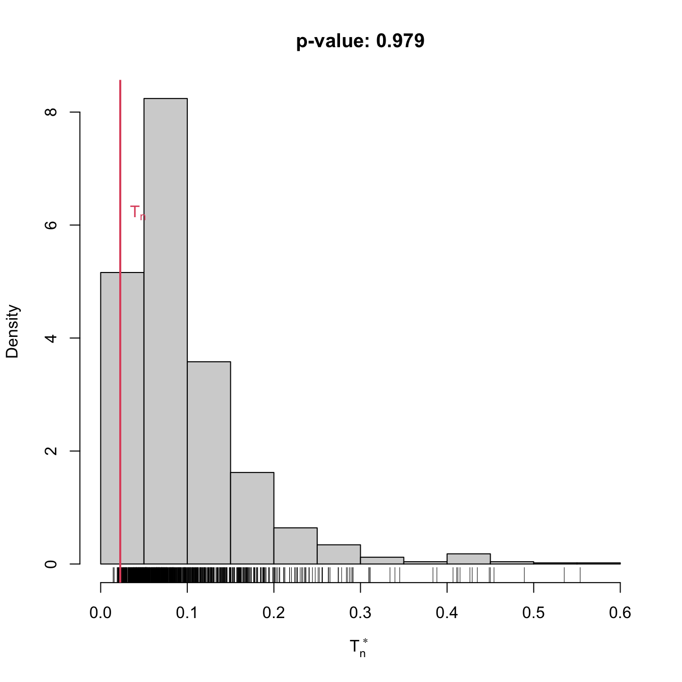

gof0
## 
##  Bootstrap-based Cramér-von Mises test for exponentiality
## 
## data:  x
## stat.omega2 = 0.022601, p-value = 0.979
## alternative hypothesis: any alternative to exponentiality

# Check the test for H0 false
x <- rgamma(n = 100, shape = 2, scale = 1)
gof1 <- cvm_exp_gof(x = x, B = 1e3)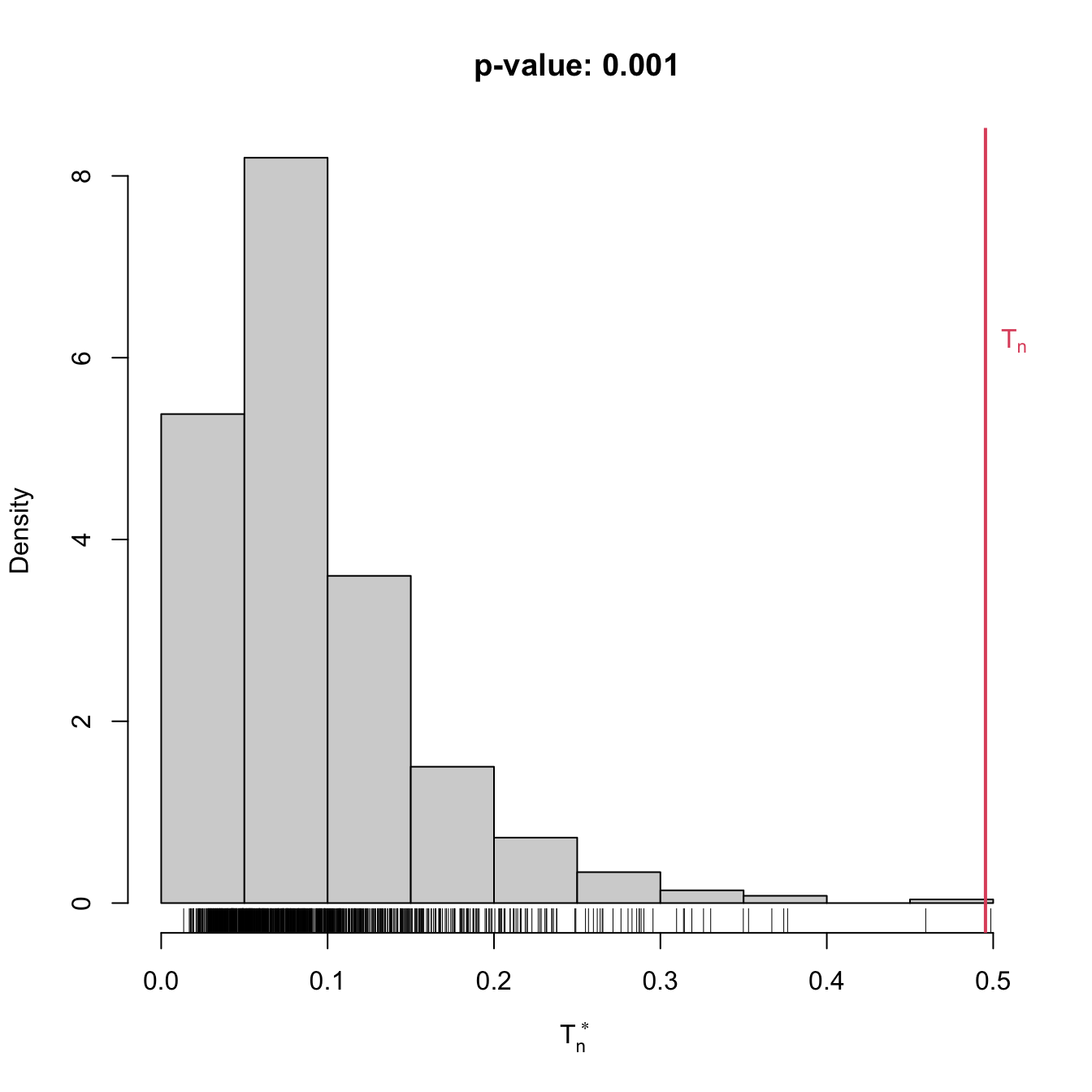

gof1
## 
##  Bootstrap-based Cramér-von Mises test for exponentiality
## 
## data:  x
## stat.omega2 = 0.49536, p-value = 0.001
## alternative hypothesis: any alternative to exponentiality

Another example is given below. It adapts the previous template for the flexible class of mixtures of normal distributions given in (2.32).

# A goodness-of-fit test of a mixture of m normals using the
# Cramér-von Mises statistic
cvm_nm_gof <- function(x, m, B = 1e3, plot_boot = TRUE) {

  # Test statistic function (depends on the data only)
  Tn <- function(data) {

    # EM algorithm for fitting normal mixtures. With trace = 0 we disable the
    # default convergence messages or otherwise they will saturate the screen
    # with the bootstrap loop. Be aware that this is a potentially dangerous
    # practice, as we may lose important information about the convergence of
    # the EM algorithm
    theta_hat <- nor1mix::norMixEM(x = data, m = m, trace = 0)

    # Test statistic
    goftest::cvm.test(x = data, null = nor1mix::pnorMix,
                      obj = theta_hat)$statistic

  }

  # Function to simulate bootstrap samples X_1^*, ..., X_n^*. Requires TWO
  # arguments, one being the data X_1, ..., X_n and the other containing
  # the parameter theta
  r_mod <- function(data, theta) {

    nor1mix::rnorMix(n = length(data), obj = theta)

  }

  # Estimate of theta
  theta_hat <- nor1mix::norMixEM(x = x, m = m, trace = 0)

  # Perform bootstrap resampling with the aid of boot::boot
  Tn_star <- boot::boot(data = x, statistic = Tn, sim = "parametric",
                        ran.gen = r_mod, mle = theta_hat, R = B)

  # Test information
  method <- "Bootstrap-based Cramér-von Mises test for normal mixtures"
  alternative <- paste("any alternative to a", m, "normal mixture")

  # p-value: modify if rejection does not happen for large values of the
  # test statistic. $t0 is the original statistic and $t has the bootstrapped
  # ones.
  pvalue <- mean(Tn_star$t > Tn_star$t0)

  # Construct an "htest" result
  result <- list(statistic = c("stat" = Tn_star$t0), p.value = pvalue,
                 theta_hat = theta_hat, statistic_boot = drop(Tn_star$t),
                 B = B, alternative = alternative, method = method,
                 data.name = deparse(substitute(x)))
  class(result) <- "htest"

  # Plot the position of the original statistic with respect to the
  # bootstrap replicates?
  if (plot_boot) {

    hist(result$statistic_boot, probability = TRUE,
         main = paste("p-value:", result$p.value),
         xlab = latex2exp::TeX("$T_n^*$"))
    rug(result$statistic_boot)
    abline(v = result$statistic, col = 2, lwd = 2)
    text(x = result$statistic, y = 1.5 * mean(par()$usr[3:4]),
         labels = latex2exp::TeX("$T_n$"), col = 2, pos = 4)

  }

  # Return "htest"
  return(result)

}

# Check the test for H0 true
set.seed(123456)
x <- c(rnorm(n = 100, mean = 2, sd = 0.5), rnorm(n = 100, mean = -2))
gof0 <- cvm_nm_gof(x = x, m = 2, B = 1e3)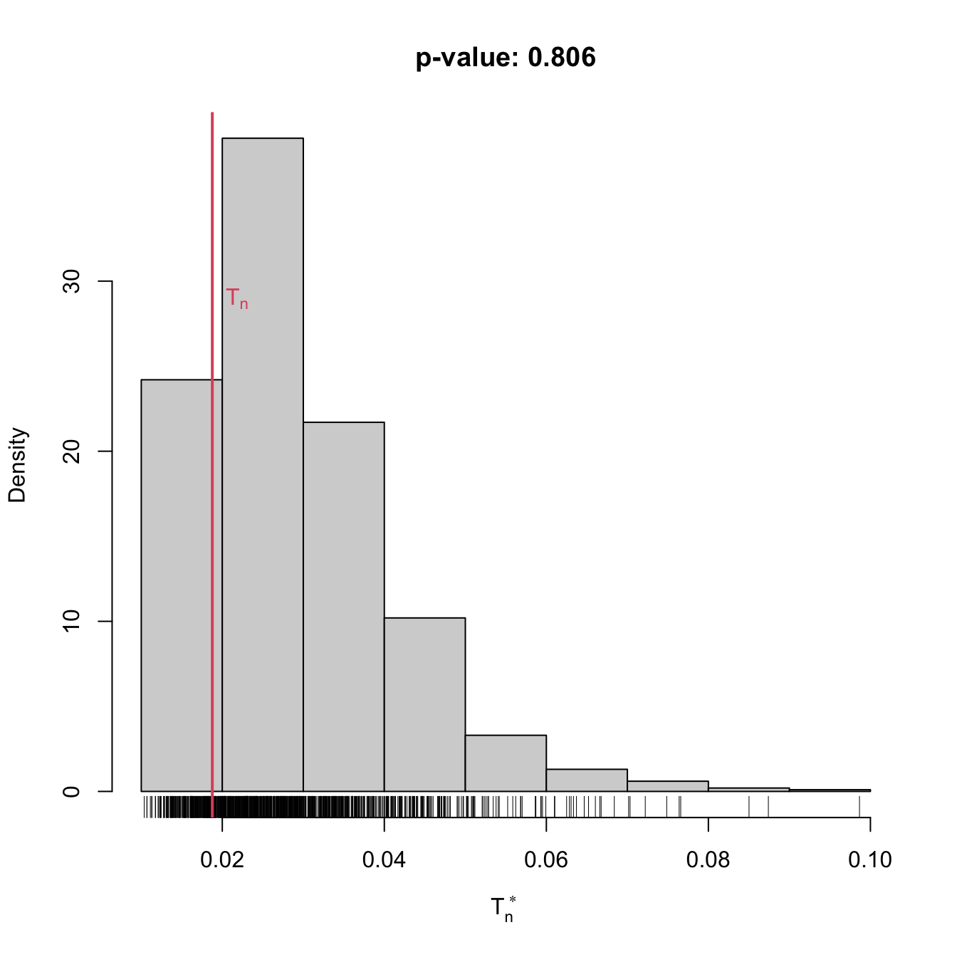

gof0
## 
##  Bootstrap-based Cramér-von Mises test for normal mixtures
## 
## data:  x
## stat.omega2 = 0.018769, p-value = 0.806
## alternative hypothesis: any alternative to a 2 normal mixture

# Graphical assessment that H0 (parametric fit) and data (kde) match
plot(gof0$theta_hat, p.norm = FALSE, ylim = c(0, 0.5))
plot(ks::kde(x), col = 2, add = TRUE)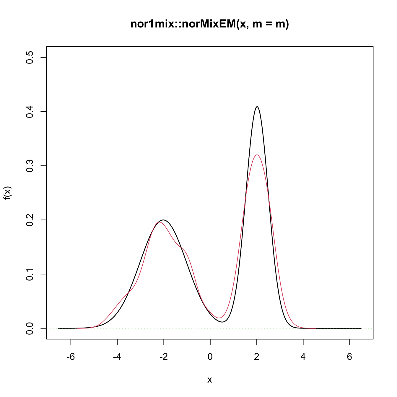


# Check the test for H0 false
x <- rgamma(n = 100, shape = 2, scale = 1)
gof1 <- cvm_nm_gof(x = x, m = 1, B = 1e3)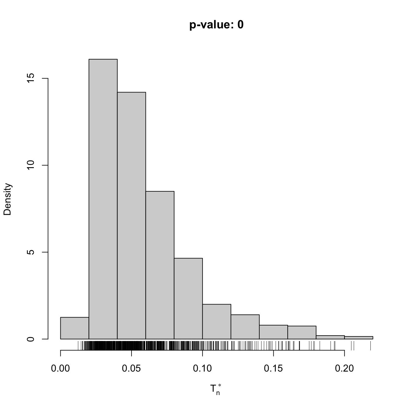

gof1
## 
##  Bootstrap-based Cramér-von Mises test for normal mixtures
## 
## data:  x
## stat.omega2 = 0.44954, p-value < 2.2e-16
## alternative hypothesis: any alternative to a 1 normal mixture

# Graphical assessment that H0 (parametric fit) and data (kde) do not match
plot(gof1$theta_hat, p.norm = FALSE, ylim = c(0, 0.5))
plot(ks::kde(x), col = 2, add = TRUE)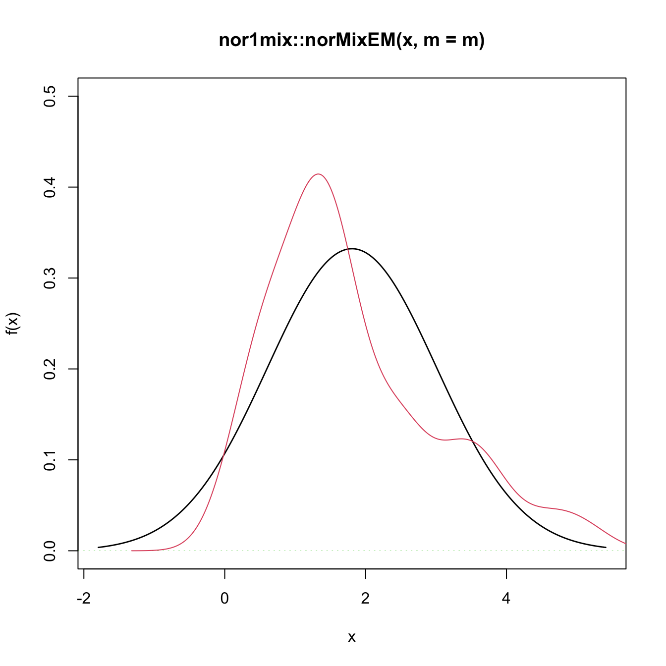

Exercise 6.10 Change in the previous example the number of mixture components to $m=3$ and $m=10,$ using the same sample as in the example. Do you reject the null hypothesis? Why? What about $m=1$? Try with new simulated datasets.

Exercise 6.11 Adapt the previous template to perform the following tasks:

Test the goodness-of-fit of the Weibull distribution using the Anderson–Darling statistic. Check with a small simulation study that the test is correctly implemented (such that the significance level $\alpha$ is respected if $H_0$ holds).
Test the goodness-of-fit of the lognormal distribution using the Anderson–Darling statistic. Check with a small simulation study that the test is correctly implemented.
Apply the previous two tests to inspect if av_gray_one from Exercise 2.25 and if temps-other.txt are distributed according to a Weibull or lognormal. Explain the results.

6.2 Comparison of two distributions

Assume that two iid samples $X_1,\ldots,X_n$ and $Y_1,\ldots,Y_m$ arbitrary distributions $F$ and $G$ are given. We next address the two-sample problem of comparing the unknown distributions $F$ and $G.$

6.2.1 Homogeneity tests

The comparison of $F$ and $G$ can be done by testing their equality, which is known as the testing for homogeneity of the samples $X_1,\ldots,X_n$ and $Y_1,\ldots,Y_m.$ We can therefore address the two-sided hypothesis test

\[\begin{align} H_0:F=G\quad\text{vs.}\quad H_1:F\neq G.\tag{6.13} \end{align}\]

Recall that, differently from the simple and composite hypothesis that appears in goodness-of-fit problems, in the homogeneity problem the null hypothesis $H_0:F=G$ does not specify any form for the distributions $F$ and $G,$ only their equality.

The one-sided hypothesis in which $H_1:F<G$ (or $H_1:F>G$) is also very relevant. Here and henceforth “$F<G$” has a special meaning:

“$F<G$”: there exists at least one $x\in\mathbb{R}$ such that $F(x)<G(x).$²³²

Obviously, the alternative $H_1:F<G$ is implied if, for all $x\in\mathbb{R},$

\[\begin{align} F(x)<G(x)&\iff \mathbb{P}[X\leq x]<\mathbb{P}[Y\leq x]\nonumber\\ &\iff \mathbb{P}[X>x]>\mathbb{P}[Y>x].\tag{6.14} \end{align}\]

Consequently, (6.14) means that $X$ produces observations above any fixed threshold $x\in\mathbb{R}$ more likely than $Y$. This concept is known as (strict)²³³ stochastic dominance and, precisely, it is said that $X$ is stochastically greater than $Y$ if (6.14) holds.²³⁴

Stochastic dominance is an intuitive concept to interpret $H_1:F<G,$ although it is a stronger statement on the relation of $F$ and $G.$ A more accurate, yet still intuitive, way of regarding $H_1:F<G$ is as a local stochastic dominance: $X$ is stochastically greater than $Y$ only for some specific thresholds $x\in\mathbb{R}.$²³⁵ Figures 6.6 and 6.8 give two examples of presence/absence of stochastic dominance where $H_1:F<G$ holds.

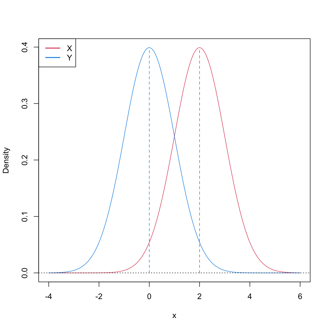
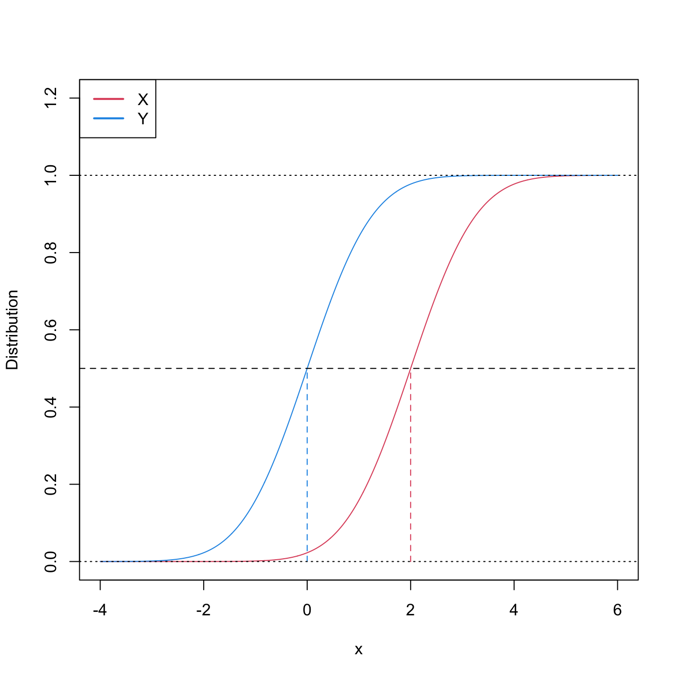
$Pdfs and cdfs of $X\sim\mathcal{N}(2,1)$ and $Y\sim\mathcal{N}(0,1).$ $X$ is stochastically greater than $Y,$ which is visualized in terms of the pdfs (shift in the mean) and cdfs (domination of $Y$’s cdf). The means are shown in solid vertical lines. Note that the variances of $X$ and $Y$ are common; compare this situation with Figure 6.8.$ $Pdfs and cdfs of $X\sim\mathcal{N}(2,1)$ and $Y\sim\mathcal{N}(0,1).$ $X$ is stochastically greater than $Y,$ which is visualized in terms of the pdfs (shift in the mean) and cdfs (domination of $Y$’s cdf). The means are shown in solid vertical lines. Note that the variances of $X$ and $Y$ are common; compare this situation with Figure 6.8.$

Figure 6.6: Pdfs and cdfs of $X\sim\mathcal{N}(2,1)$ and $Y\sim\mathcal{N}(0,1).$ $X$ is stochastically greater than $Y,$ which is visualized in terms of the pdfs (shift in the mean) and cdfs (domination of $Y$’s cdf). The means are shown in solid vertical lines. Note that the variances of $X$ and $Y$ are common; compare this situation with Figure 6.8.

The ecdf-based goodness-of-fit tests seen in Section 6.1.1 can be adapted to the homogeneity problem, with varying difficulty and versatility. The two-sample Kolmogorov–Smirnov test offers the highest simplicity and versatility, yet its power is inferior to that of the two-sample Cramér–von Mises and Anderson–Darling tests.

6.2.1.1 Two-sample Kolmogorov–Smirnov test (two-sided)

Test purpose. Given $X_1,\ldots,X_n\sim F$ and $Y_1,\ldots,Y_m\sim G,$ it tests $H_0: F=G$ vs. $H_1: F\neq G$ consistently against all the alternatives in $H_1.$
Statistic definition. The test statistic uses the supremum distance between $F_n$ and $G_m$:²³⁶

\[\begin{align*} D_{n,m}:=\sqrt{\frac{nm}{n+m}}\sup_{x\in\mathbb{R}} \left|F_n(x)-G_m(x)\right|. \end{align*}\]

If $H_0:F=G$ holds, then $D_{n,m}$ tends to be small. Conversely, when $F\neq G,$ larger values of $D_{n,m}$ are expected, and the test rejects $H_0$ when $D_{n,m}$ is large.
Statistic computation. The computation of $D_{n,m}$ can be efficiently achieved by realizing that the maximum difference between $F_n$ and $G_m$ happens at $x=X_i$ or $x=Y_j,$ for a certain $X_i$ or $Y_j$ (observe Figure 6.7). Therefore,

\[\begin{align} D_{n,m}=&\,\max(D_{n,m,1},D_{n,m,2}),\tag{6.15}\\ D_{n,m,1}:=&\,\sqrt{\frac{nm}{n+m}}\max_{1\leq i\leq n}\left|\frac{i}{n}-G_m(X_{(i)})\right|,\nonumber\\ D_{n,m,2}:=&\,\sqrt{\frac{nm}{n+m}}\max_{1\leq j\leq m}\left|F_n(Y_{(j)})-\frac{j}{m}\right|.\nonumber \end{align}\]
Distribution under $H_0.$ If $H_0$ holds and $F=G$ is continuous, then $D_{n,m}$ has the same asymptotic cdf as $D_n$ (check (6.3)).²³⁷ That is,

\[\begin{align*} \lim_{n,m\to\infty}\mathbb{P}[D_{n,m}\leq x]=K(x). \end{align*}\]
Highlights and caveats. The two-sample Kolmogorov–Smirnov test is distribution-free if $F=G$ is continuous and the samples $X_1,\ldots,X_n$ and $Y_1,\ldots,Y_m$ have no ties. If these assumptions are met, then the iid sample $X_1,\ldots,X_n,Y_1,\ldots,Y_m\stackrel{H_0}{\sim} F=G$ generates the iid sample $U_1,\ldots,U_{n+m}\stackrel{H_0}{\sim} \mathcal{U}(0,1),$ where $U_i:=F(X_i)$ and $U_{n+j}:=G(Y_j),$ for $i=1,\ldots,n,$ $j=1,\ldots,m.$ As a consequence, the distribution of (6.2) does not depend on $F=G.$ If $F=G$ is not continuous or there are ties on the sample, the $K$ function is not the true asymptotic distribution.
Implementation in R. For continuous data and continuous $F=G,$ the test statistic $D_{n,m}$ and the asymptotic $p$-value are readily available through the ks.test function (with its default alternative = "two-sided"). For discrete $F=G,$ a test implementation can be achieved through the permutation approach to be seen in Section 6.2.3.

The construction of the two-sample Kolmogorov–Smirnov test statistic is illustrated in the following chunk of code.

# Sample data
n <- 10; m <- 10
mu1 <- 0; sd1 <- 1
mu2 <- 0; sd2 <- 2
set.seed(1998)
samp1 <- rnorm(n = n, mean = mu1, sd = sd1)
samp2 <- rnorm(n = m, mean = mu2, sd = sd2)

# Fn vs. Gm
plot(ecdf(samp1), main = "", ylab = "Probability", xlim = c(-3.5, 3.5),
     ylim = c(0, 1.3))
lines(ecdf(samp2), main = "", col = 4)

# Add Dnm1
samp1_sorted <- sort(samp1)
samp2_sorted <- sort(samp2)
Dnm_1 <- abs((1:n) / n - ecdf(samp2)(samp1_sorted))
i1 <- which.max(Dnm_1)
lines(rep(samp2_sorted[i1], 2),
      c(i1 / m, ecdf(samp1_sorted)(samp2_sorted[i1])),
      col = 3, lwd = 2, type = "o", pch = 16, cex = 0.75)
rug(samp1, col = 1)

# Add Dnm2
Dnm_2 <- abs(ecdf(samp1)(samp2_sorted) - (1:m) / m)
i2 <- which.max(Dnm_2)
lines(rep(samp1_sorted[i2], 2),
      c(i2 / n, ecdf(samp2_sorted)(samp1_sorted[i2])),
      col = 2, lwd = 2, type = "o", pch = 16, cex = 0.75)
rug(samp2, col = 4)
legend("topleft", lwd = 2, col = c(1, 4, 3, 2), legend =
         latex2exp::TeX(c("$F_n$", "$G_m$", "$D_{n,m,1}$", "$D_{n,m,2}$")))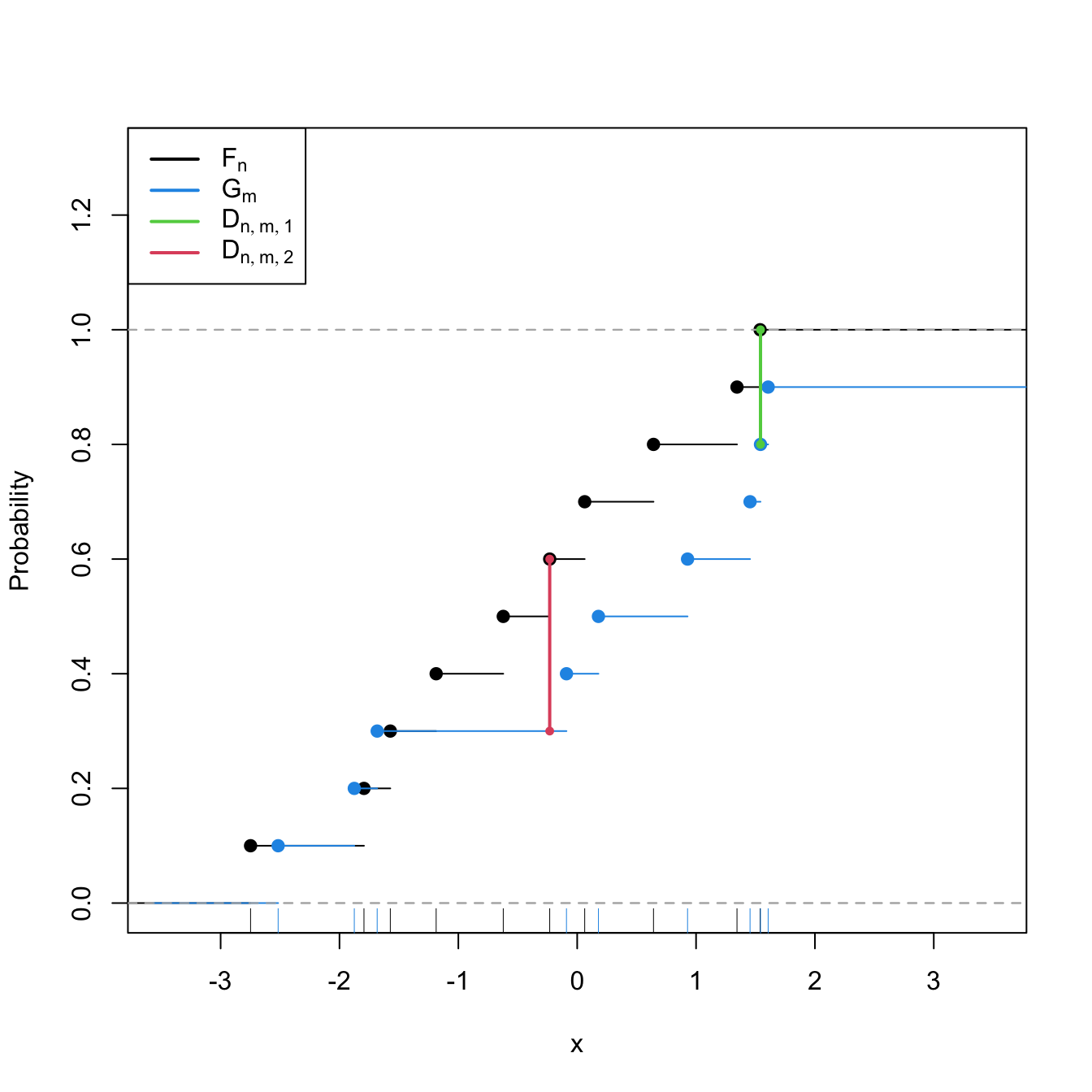

$Kolmogorov–Smirnov distance $D_{n,m}=\max(D_{n,m,1},D_{n,m,2})$ for two samples of sizes $n=m=10$ coming from $F(\cdot)=\Phi\left(\frac{\cdot-\mu_1}{\sigma_1}\right)$ and $G(\cdot)=\Phi\left(\frac{\cdot-\mu_2}{\sigma_2}\right),$ where $\mu_1=\mu_2=0,$ and $\sigma_1=1$ and $\sigma_2=2.$$

Figure 6.7: Kolmogorov–Smirnov distance $D_{n,m}=\max(D_{n,m,1},D_{n,m,2})$ for two samples of sizes $n=m=10$ coming from $F(\cdot)=\Phi\left(\frac{\cdot-\mu_1}{\sigma_1}\right)$ and $G(\cdot)=\Phi\left(\frac{\cdot-\mu_2}{\sigma_2}\right),$ where $\mu_1=\mu_2=0,$ and $\sigma_1=1$ and $\sigma_2=2.$

An instance of the use of the ks.test function for the two-sided homogeneity test is given below.

# Check the test for H0 true
set.seed(123456)
x0 <- rgamma(n = 50, shape = 1, scale = 1)
y0 <- rgamma(n = 100, shape = 1, scale = 1)
ks.test(x = x0, y = y0)
## 
##  Exact two-sample Kolmogorov-Smirnov test
## 
## data:  x0 and y0
## D = 0.14, p-value = 0.5185
## alternative hypothesis: two-sided

# Check the test for H0 false
x1 <- rgamma(n = 50, shape = 2, scale = 1)
y1 <- rgamma(n = 75, shape = 1, scale = 1)
ks.test(x = x1, y = y1)
## 
##  Exact two-sample Kolmogorov-Smirnov test
## 
## data:  x1 and y1
## D = 0.35333, p-value = 0.0008513
## alternative hypothesis: two-sided

6.2.1.2 Two-sample Kolmogorov–Smirnov test (one-sided)

Test purpose. Given $X_1,\ldots,X_n\sim F$ and $Y_1,\ldots,Y_m\sim G,$ it tests $H_0: F=G$ vs. $H_1: F<G.$²³⁸ Rejection of $H_0$ in favor of $H_1$ gives evidence for the local stochastic dominance of $X$ over $Y$ (which may or may not be global).
Statistic definition. The test statistic uses the maximum signed distance between $F_n$ and $G_m$:

\[\begin{align*} D_{n,m}^-:=\sqrt{\frac{nm}{n+m}}\sup_{x\in\mathbb{R}} (G_m(x)-F_n(x)). \end{align*}\]

If $H_1:F<G$ holds, then $D_{n,m}^-$ tends to have large positive values. Conversely, when $H_0:F=G$ or $F>G$ holds, smaller values of $D_{n,m}^-$ are expected, possibly negative. The test rejects $H_0$ when $D_{n,m}^-$ is large.
Statistic computation. The computation of $D_{n,m}^-$ is analogous to that of $D_{n,m}$ given in (6.15), but removing absolute values and changing its sign:²³⁹

\[\begin{align*} D_{n,m}^-=&\,\max(D_{n,m,1}^-,D_{n,m,2}^-),\\ D_{n,m,1}^-:=&\,\sqrt{\frac{nm}{n+m}}\max_{1\leq i\leq n}\left(G_m(X_{(i)})-\frac{i}{n}\right),\\ D_{n,m,2}^-:=&\,\sqrt{\frac{nm}{n+m}}\max_{1\leq j\leq m}\left(\frac{j}{m}-F_n(Y_{(j)})\right). \end{align*}\]
Distribution under $H_0.$ If $H_0$ holds and $F=G$ is continuous, then $D_{n,m}^-$ has the same asymptotic cdf as $D_{n,m}$.
Highlights and caveats. The one-sided two-sample Kolmogorov–Smirnov test is also distribution-free if $F=G$ is continuous and the samples $X_1,\ldots,X_n$ and $Y_1,\ldots,Y_m$ have no ties.
Implementation in R. For continuous data and continuous $F=G,$ the test statistic $D_{n,m}^-$ and the asymptotic $p$-value are readily available through the ks.test function. The one-sided test is carried out if alternative = "less" or alternative = "greater" (not the defaults). The argument alternative means the direction of cdf dominance: "less" $\equiv F\boldsymbol{<}G;$ "greater" $\equiv F\boldsymbol{>}G.$²⁴⁰ $\!\!^,$²⁴¹ Permutations (see Section 6.2.3) can be used for obtaining non-asymptotic $p$-values and dealing with discrete samples.

# Check the test for H0 true
set.seed(123456)
x0 <- rgamma(n = 50, shape = 1, scale = 1)
y0 <- rgamma(n = 100, shape = 1, scale = 1)
ks.test(x = x0, y = y0, alternative = "less") # H1: F < G
## 
##  Exact two-sample Kolmogorov-Smirnov test
## 
## data:  x0 and y0
## D^- = 0.08, p-value = 0.643
## alternative hypothesis: the CDF of x lies below that of y
ks.test(x = x0, y = y0, alternative = "greater") # H1: F > G
## 
##  Exact two-sample Kolmogorov-Smirnov test
## 
## data:  x0 and y0
## D^+ = 0.14, p-value = 0.2638
## alternative hypothesis: the CDF of x lies above that of y

# Check the test for H0 false
x1 <- rnorm(n = 50, mean = 1, sd = 1)
y1 <- rnorm(n = 75, mean = 0, sd = 1)
ks.test(x = x1, y = y1, alternative = "less") # H1: F < G
## 
##  Exact two-sample Kolmogorov-Smirnov test
## 
## data:  x1 and y1
## D^- = 0.52667, p-value = 2.205e-08
## alternative hypothesis: the CDF of x lies below that of y
ks.test(x = x1, y = y1, alternative = "greater") # H1: F > G
## 
##  Exact two-sample Kolmogorov-Smirnov test
## 
## data:  x1 and y1
## D^+ = 1.4502e-15, p-value = 1
## alternative hypothesis: the CDF of x lies above that of y
# Interpretations:
# 1. Strong rejection of H0: F = G in favor of H1: F < G when
# alternative = "less", as in reality x1 is stochastically greater than y1.
# This outcome allows stating that "there is strong evidence supporting that
# x1 is locally stochastically greater than y1"
# 2. No rejection ("strong acceptance") of H0: F = G versus H1: F > G when
# alternative = "greater". Even if in reality x1 is stochastically greater than
# y1 (so H0 is false), the alternative to which H0 is confronted is even less
# plausible. A p-value ~ 1 indicates that one is probably conducting the test
# in the uninteresting direction alternative!

Exercise 6.12 Consider the two populations described in Figure 6.8. $X\sim F$ is not stochastically greater than $Y\sim G.$ However, $Y$ is locally stochastically greater than $X$ in $(-\infty,-0.75).$ Therefore, although hard to detect, the two-sample Kolmogorov–Smirnov test should eventually reject $H_0:F=G$ in favor of $H_1:F>G.$ Conduct a simulation study to verify how fast this rejection takes place:

Simulate $X_1,\ldots,X_n\sim F$ and $Y_1,\ldots,Y_n\sim G.$
Apply ks.test with the corresponding alternative and evaluate if it rejects $H_0$ at a significance level $\alpha.$
Repeat Steps 1–2 $M=100$ times and approximate the rejection probability by Monte Carlo.
Perform Steps 1–3 for a suitably increasing sequence of sample sizes $n,$ then plot the estimated power as a function of $n.$ Consider a sequence of sample sizes that shows the power curve converging to one.
Compare the previous curve against the rejection probability curves for $H_1:F<G$ and $H_1:F\neq G.$
Once you have a working solution, increase $M$ to $M=1,000.$
Summarize your conclusions.

6.2.1.3 Two-sample Cramér–von Mises test

Test purpose. Given $X_1,\ldots,X_n\sim F,$ it tests $H_0: F=G$ vs. $H_1: F\neq G$ consistently against all the alternatives in $H_1.$
Statistic definition. The test statistic proposed by Anderson (1962) uses a quadratic distance between $F_n$ and $G_m$:

\[\begin{align} W_{n,m}^2:=\frac{nm}{n+m}\int(F_n(z)-G_m(z))^2\,\mathrm{d}H_{n+m}(z),\tag{6.16} \end{align}\]

where $H_{n+m}$ is the ecdf of the pooled sample $Z_1,\ldots,Z_{n+m},$ where $Z_i:=X_i$ and $Z_{j+n}:=Y_j,$ $i=1,\ldots,n$ and $j=1,\ldots,m.$²⁴² Therefore, $H_{n+m}(z)=\frac{n}{n+m}F_n(z)+\frac{m}{n+m}G_m(z),$ $z\in\mathbb{R},$ and (6.16) equals²⁴³

\[\begin{align} W_{n,m}^2=\frac{nm}{(n+m)^2}\sum_{k=1}^{n+m}(F_n(Z_k)-G_m(Z_k))^2.\tag{6.17} \end{align}\]
Statistic computation. The formula (6.17) is reasonably direct. Better computational efficiency may be obtained with ranks from the pooled sample.
Distribution under $H_0.$ If $H_0$ holds and $F=G$ is continuous, then $W_{n,m}^2$ has the same asymptotic cdf as $W_n^2$ (see (6.6)).
Highlights and caveats. The two-sample Cramér–von Mises test is also distribution-free if $F=G$ is continuous and the sample has no ties. Otherwise, (6.6) is not the true asymptotic distribution. As in the one-sample case, empirical evidence suggests that the Cramér–von Mises test is often more powerful than the Kolmogorov–Smirnov test. However, the Cramér–von Mises is less versatile, since it does not admit simple modifications to test against one-sided alternatives.
Implementation in R. See below for the statistic implementation. Asymptotic $p$-values can be obtained using goftest::pCvM. Permutations (see Section 6.2.3) can be used for obtaining non-asymptotic $p$-values and dealing with discrete samples.

# Two-sample Cramér-von Mises statistic
cvm2_stat <- function(x, y) {

  # Sample sizes
  n <- length(x)
  m <- length(y)

  # Pooled sample
  z <- c(x, y)

  # Statistic computation via ecdf()
  (n * m / (n + m)^2) * sum((ecdf(x)(z) - ecdf(y)(z))^2)

}

# Check the test for H0 true
set.seed(123456)
x0 <- rgamma(n = 50, shape = 1, scale = 1)
y0 <- rgamma(n = 100, shape = 1, scale = 1)
cvm0 <- cvm2_stat(x = x0, y = y0)
pval0 <- 1 - goftest::pCvM(q = cvm0)
c("statistic" = cvm0, "p-value"= pval0)
## statistic   p-value 
## 0.1294889 0.4585971

# Check the test for H0 false
x1 <- rgamma(n = 50, shape = 2, scale = 1)
y1 <- rgamma(n = 75, shape = 1, scale = 1)
cvm1 <- cvm2_stat(x = x1, y = y1)
pval1 <- 1 - goftest::pCvM(q = cvm1)
c("statistic" = cvm1, "p-value"= pval1)
##    statistic      p-value 
## 1.3283733333 0.0004264598

6.2.1.4 Two-sample Anderson–Darling test

Test purpose. Given $X_1,\ldots,X_n\sim F,$ it tests $H_0: F=G$ vs. $H_1: F\neq G$ consistently against all the alternatives in $H_1.$
Statistic definition. The test statistic proposed by Pettitt (1976) uses a weighted quadratic distance between $F_n$ and $G_m$:

\[\begin{align} A_{n,m}^2:=\frac{nm}{n+m}\int\frac{(F_n(z)-G_m(z))^2}{H_{n+m}(z)(1-H_{n+m}(z))}\,\mathrm{d}H_{n+m}(z),\tag{6.18} \end{align}\]

where $H_{n+m}$ is the ecdf of $Z_1,\ldots,Z_{n+m}.$ Therefore, (6.18) equals

\[\begin{align} A_{n,m}^2=\frac{nm}{(n+m)^2}\sum_{k=1}^{n+m}\frac{(F_n(Z_k)-G_m(Z_k))^2}{H_{n+m}(Z_k)(1-H_{n+m}(Z_k))}.\tag{6.19} \end{align}\]

In (6.19), it is implicitly assumed that the largest observation of the pooled sample, $Z_{(n+m)},$ is excluded from the sum, since $H_{n+m}(Z_{(n+m)})=1.$²⁴⁴
Statistic computation. The formula (6.19) is reasonably direct for computation. Better computational efficiency may be obtained with ranks from the pooled sample. The implicit exclusion of $Z_{(n+m)}$ from the sum in (6.19) can be made explicit with

\[\begin{align*} A_{n,m}^2=\frac{nm}{(n+m)^2}\sum_{k=1}^{n+m-1}\frac{(F_n(Z_{(k)})-G_m(Z_{(k)}))^2}{H_{n+m}(Z_{(k)})(1-H_{n+m}(Z_{(k)}))}. \end{align*}\]
Distribution under $H_0.$ If $H_0$ holds and $F=G$ is continuous, then $A_{n,m}^2$ has the same asymptotic cdf as $A_n^2$ (see (6.8)).
Highlights and caveats. The two-sample Anderson–Darling test is also distribution-free if $F=G$ is continuous and the sample has no ties. Otherwise, (6.8) is not the true asymptotic distribution. As in the one-sample case, empirical evidence suggests that the Anderson–Darling test is often more powerful than the Kolmogorov–Smirnov and Cramér–von Mises tests. The two-sample Anderson–Darling test is also less versatile, since it does not admit simple modifications to test against one-sided alternatives.
Implementation in R. See below for the statistic implementation. Asymptotic $p$-values can be obtained using goftest::pAD. Permutations (see Section 6.2.3) can be used for obtaining non-asymptotic $p$-values and dealing with discrete samples.

# Two-sample Anderson-Darling statistic
ad2_stat <- function(x, y) {

  # Sample sizes
  n <- length(x)
  m <- length(y)

  # Pooled sample and pooled ecdf
  z <- c(x, y)
  z <- z[-which.max(z)] # Exclude the largest point
  H <- rank(z) / (n + m)

  # Statistic computation via ecdf()
  (n * m / (n + m)^2) * sum((ecdf(x)(z) - ecdf(y)(z))^2 / ((1 - H) * H))

}

# Check the test for H0 true
set.seed(123456)
x0 <- rgamma(n = 50, shape = 1, scale = 1)
y0 <- rgamma(n = 100, shape = 1, scale = 1)
ad0 <- ad2_stat(x = x0, y = y0)
pval0 <- 1 - goftest::pAD(q = ad0)
c("statistic" = ad0, "p-value"= pval0)
## statistic   p-value 
## 0.8603617 0.4394751

# Check the test for H0 false
x1 <- rgamma(n = 50, shape = 2, scale = 1)
y1 <- rgamma(n = 75, shape = 1, scale = 1)
ad1 <- ad2_stat(x = x1, y = y1)
pval1 <- 1 - goftest::pAD(q = ad1)
c("statistic" = ad1, "p-value"= pval1)
##    statistic      p-value 
## 6.7978295422 0.0004109238

Exercise 6.13 Verify the correctness of the asymptotic null distributions of $W_{n,m}^2$ and $A_{n,m}^2.$ To do so:

Simulate $M=1,000$ pairs of samples of sizes $n=200$ and $m=150$ under $H_0.$
Obtain the statistics $W_{n,m;1}^2,\ldots, W_{n,m;M}^2$ and plot their ecdf.
Overlay the asymptotic cdf of $W_{n,m},$ provided by goftest::pCvM for the one-sample test.
Repeat Steps 2–3 for $A_{n,m}^2.$

Exercise 6.14 Implement in R a single function to properly conduct either the two-sample Cramér–von Mises test or the two-sample Anderson–Darling test. The function must return a tidied "htest" object. Is your implementation of $W_{n,m}^2$ and $A_{n,m}^2$ able to improve cvm2_stat and ad2_stat in speed? Measure the running times for $n=300$ and $m=200$ with the microbenchmark::microbenchmark function.

6.2.2 Specific tests for distribution shifts

Among the previous ecdf-based tests of homogeneity, only the two-sample Kolmogorov–Smirnov test was able to readily deal with one-sided alternatives. However, this test is often more conservative than the Cramér–von Mises and the Anderson–Darling, so it is apparent that there is room for improvement. We next see two nonparametric tests, the Wilcoxon–Mann–Whitney test²⁴⁵ and the Wilcoxon signed-rank test,²⁴⁶ which are designed to detect one-sided alternatives related to $X$ being stochastically greater than $Y$. Both tests are more powerful than the one-sided Kolmogorov–Smirnov.

In a very vague and imprecise form, these tests can be interpreted as “nonparametric $t$-tests” for unpaired and paired data.²⁴⁷ The rationale is that, very often, the aforementioned one-sided alternatives are related to differences in the distributions produced by a shift in their main masses of probability. However, as we will see, there are many subtleties and sides to the previous interpretation. Unfortunately, these nuances are usually ignored in the literature and, as a consequence, the Wilcoxon–Mann–Whitney and Wilcoxon signed-rank tests are massively misunderstood and misused.

6.2.2.1 Wilcoxon–Mann–Whitney test

The Wilcoxon–Mann–Whitney test addresses the hypothesis testing of

\[\begin{align*} H_0:F=G\quad\text{vs.}\quad H_1:\mathbb{P}[X\geq Y]>0.5. \end{align*}\]

The alternative hypothesis $H_1$ requires special care:

That $\mathbb{P}[X\geq Y]>0.5$ intuitively means that the main mass of probability of $X$ is above that of $Y$: it is more likely to observe $X\geq Y$ than $X<Y.$
$H_1$ is related to $X$ being stochastically greater than $Y.$ Precisely, $H_1$ is essentially²⁴⁸ implied by the latter:

\[\begin{align*} F(x)<G(x) \text{ for all } x\in\mathbb{R} \implies \mathbb{P}[X\geq Y]\geq 0.5. \end{align*}\]

The converse implication is false (see Figure 6.8). Hence, $H_1:\mathbb{P}[X\geq Y]>0.5$ is more specific than “$X$ is stochastically greater than $Y$”. $H_1$ neither implies nor is implied by the two-sample Kolmogorov–Smirnov’s alternative $H_1':F<G$ (which can be regarded as local stochastic dominance).²⁴⁹

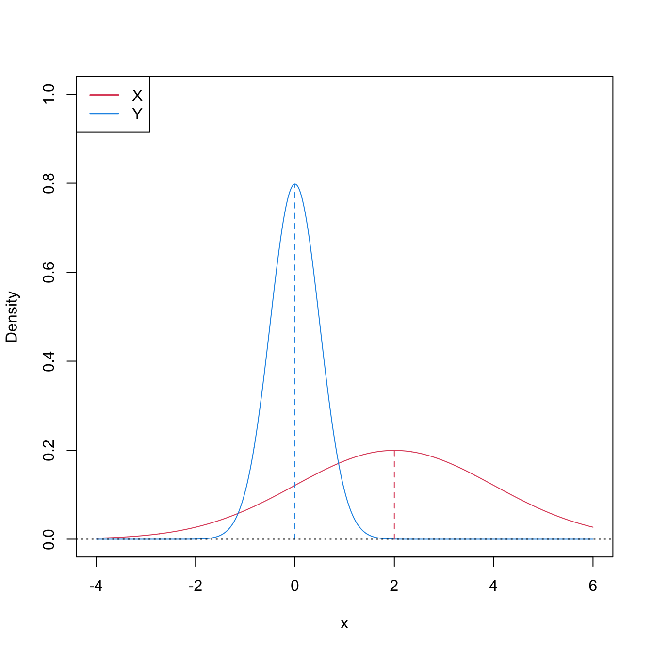
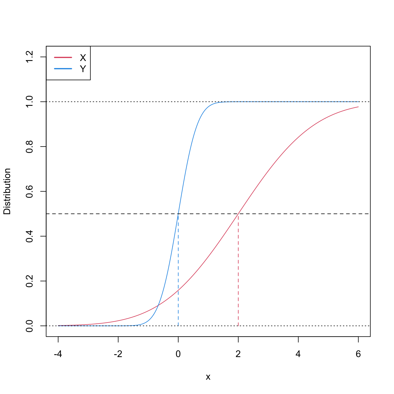
$Pdfs and cdfs of $X\sim\mathcal{N}(2,4)$ and $Y\sim\mathcal{N}(0,0.25).$ $X$ is not stochastically greater than $Y,$ as the cdfs cross, but $\mathbb{P}\lbrack X\geq Y\rbrack=0.834.$ $Y$ is locally stochastically greater than $X$ in $(-\infty,-0.75).$ The means are shown in vertical lines. Note that the variances of $X$ and $Y$ are not common; recall the difference with respect to the situation in Figure 6.6.$ $Pdfs and cdfs of $X\sim\mathcal{N}(2,4)$ and $Y\sim\mathcal{N}(0,0.25).$ $X$ is not stochastically greater than $Y,$ as the cdfs cross, but $\mathbb{P}\lbrack X\geq Y\rbrack=0.834.$ $Y$ is locally stochastically greater than $X$ in $(-\infty,-0.75).$ The means are shown in vertical lines. Note that the variances of $X$ and $Y$ are not common; recall the difference with respect to the situation in Figure 6.6.$

Figure 6.8: Pdfs and cdfs of $X\sim\mathcal{N}(2,4)$ and $Y\sim\mathcal{N}(0,0.25).$ $X$ is not stochastically greater than $Y,$ as the cdfs cross, but $\mathbb{P}\lbrack X\geq Y\rbrack=0.834.$ $Y$ is locally stochastically greater than $X$ in $(-\infty,-0.75).$ The means are shown in vertical lines. Note that the variances of $X$ and $Y$ are not common; recall the difference with respect to the situation in Figure 6.6.

In general, $H_1$ does not directly inform on the medians/means of $X$ and $Y.$ Thus, in general, the Wilcoxon–Mann–Whitney test does not compare medians/means. The probability in $H_1$ is, in general, exogenous to medians/means:²⁵⁰

\[\begin{align} \mathbb{P}[X\geq Y]=\int F_Y(x)\,\mathrm{d}F_X(x).\tag{6.20} \end{align}\]

Only in very specific circumstances $H_1$ is related to medians/means. If $X\sim F$ and $Y\sim G$ are symmetric random variables with medians $m_X$ and $m_Y$ (if the means exist, they equal the medians), then

\[\begin{align} \mathbb{P}[X\geq Y]>0.5 \iff m_X>m_Y.\tag{6.21} \end{align}\]

This characterization informs on the closest the Wilcoxon–Mann–Whitney test gets to a nonparametric version of the $t$-test.²⁵¹ However, as the two counterexamples in Figures 6.9 and 6.10 respectively illustrate, (6.21) is not true in general, neither for means nor for medians. It may happen that: (i) $\mathbb{P}[X\geq Y]>0.5$ but $\mu_X<\mu_Y;$ or (ii) $\mathbb{P}[X\geq Y]>0.5$ but $m_X<m_Y.$

$Pdfs and cdfs of $X$ and $Y\sim0.8\mathcal{N}(-3,1)+0.2\mathcal{N}(5,4),$ where $X$ is distributed as the mixture nor1mix::MW.nm3 but with its standard deviations multiplied by $5$. 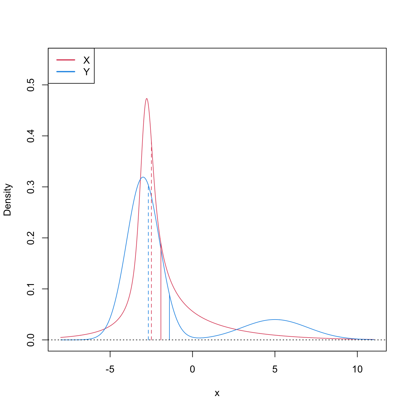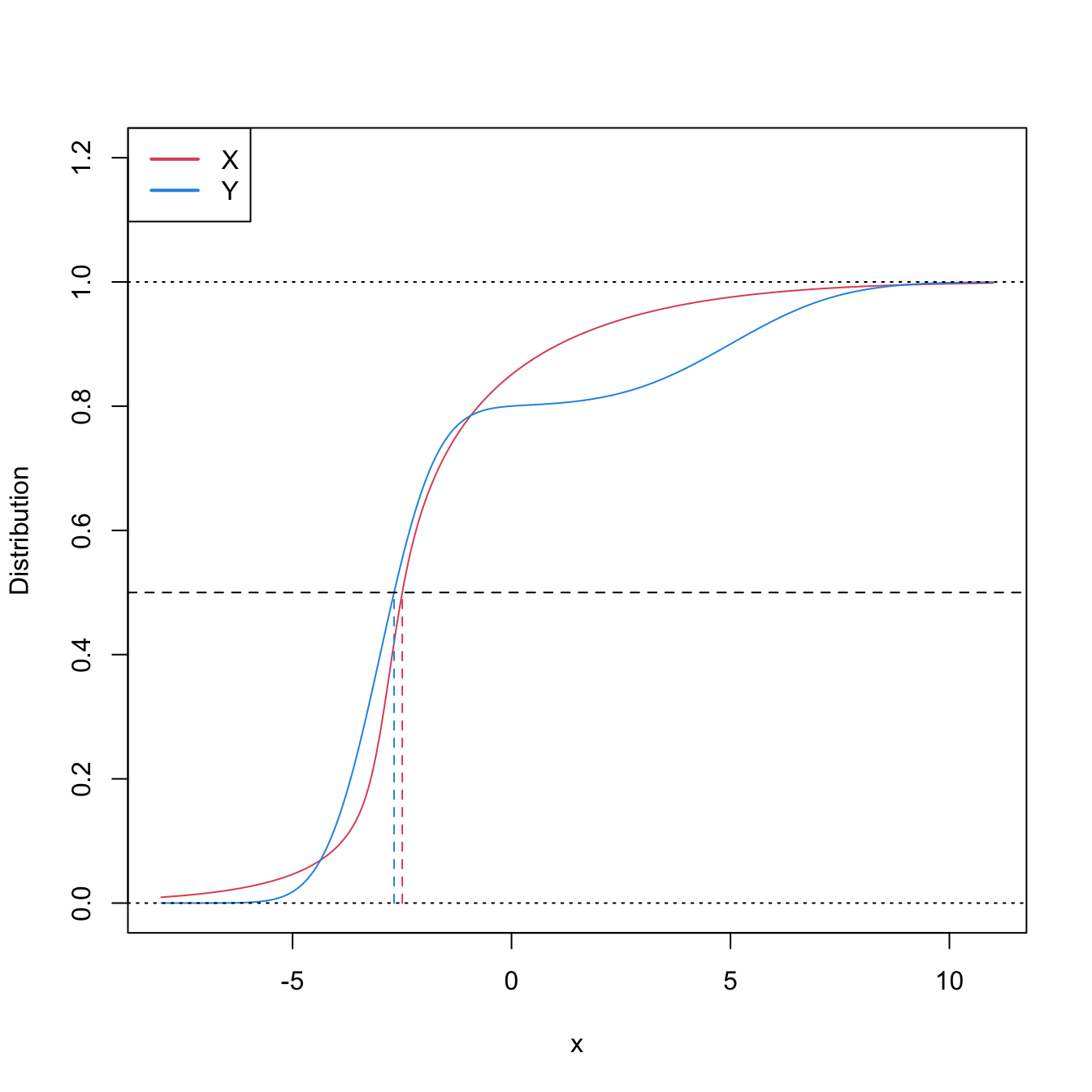$\mathbb{P}\lbrack X\geq Y\rbrack=0.5356$ but $\mu_X<\mu_Y,$ since $\mu_X=-1.9189$ and $\mu_Y=-1.4.$ The means are shown in solid vertical lines; the dashed vertical lines stand for the medians $m_X=-2.4944$ and $m_Y=-2.6814.$$ $Pdfs and cdfs of $X$ and $Y\sim0.8\mathcal{N}(-3,1)+0.2\mathcal{N}(5,4),$ where $X$ is distributed as the mixture nor1mix::MW.nm3 but with its standard deviations multiplied by $5$. $\mathbb{P}\lbrack X\geq Y\rbrack=0.5356$ but $\mu_X<\mu_Y,$ since $\mu_X=-1.9189$ and $\mu_Y=-1.4.$ The means are shown in solid vertical lines; the dashed vertical lines stand for the medians $m_X=-2.4944$ and $m_Y=-2.6814.$$

Figure 6.9: Pdfs and cdfs of $X$ and $Y\sim0.8\mathcal{N}(-3,1)+0.2\mathcal{N}(5,4),$ where $X$ is distributed as the mixture nor1mix::MW.nm3 but with its standard deviations multiplied by $5$. $\mathbb{P}\lbrack X\geq Y\rbrack=0.5356$ but $\mu_X<\mu_Y,$ since $\mu_X=-1.9189$ and $\mu_Y=-1.4.$ The means are shown in solid vertical lines; the dashed vertical lines stand for the medians $m_X=-2.4944$ and $m_Y=-2.6814.$

$Pdfs and cdfs of $X\sim0.55\mathcal{N}(-1.5,1.25^2)+0.45\mathcal{N}(7,0.75^2)$ and $Y\sim0.4\mathcal{N}(-5,1)+0.6\mathcal{N}(5,1).$ $\mathbb{P}\lbrack X\geq Y\rbrack=0.6520$ but $m_X<m_Y,$ since $m_X=0.169$ and $m_Y=4.0326.$ The medians are shown in dashed vertical lines; the means are $\mu_X=2.325$ and $\mu_Y=1.$$ $Pdfs and cdfs of $X\sim0.55\mathcal{N}(-1.5,1.25^2)+0.45\mathcal{N}(7,0.75^2)$ and $Y\sim0.4\mathcal{N}(-5,1)+0.6\mathcal{N}(5,1).$ $\mathbb{P}\lbrack X\geq Y\rbrack=0.6520$ but $m_X<m_Y,$ since $m_X=0.169$ and $m_Y=4.0326.$ The medians are shown in dashed vertical lines; the means are $\mu_X=2.325$ and $\mu_Y=1.$$

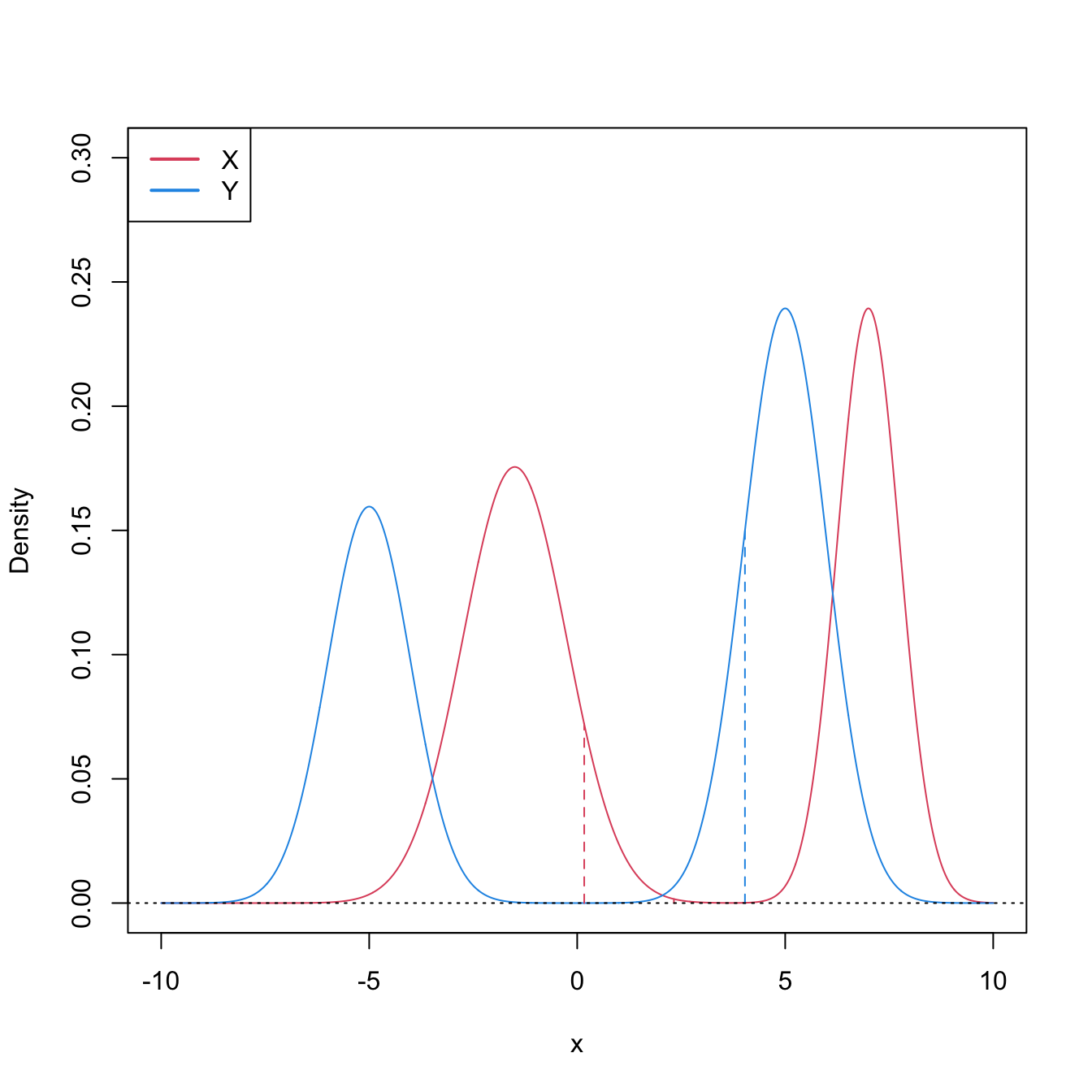
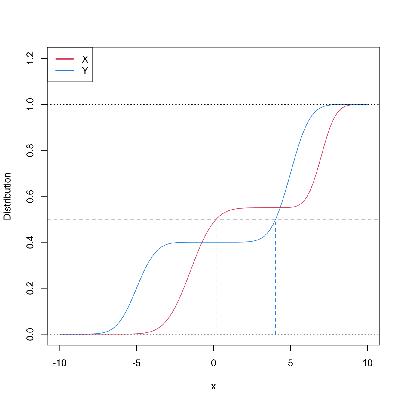
Figure 6.10: Pdfs and cdfs of $X\sim0.55\mathcal{N}(-1.5,1.25^2)+0.45\mathcal{N}(7,0.75^2)$ and $Y\sim0.4\mathcal{N}(-5,1)+0.6\mathcal{N}(5,1).$ $\mathbb{P}\lbrack X\geq Y\rbrack=0.6520$ but $m_X<m_Y,$ since $m_X=0.169$ and $m_Y=4.0326.$ The medians are shown in dashed vertical lines; the means are $\mu_X=2.325$ and $\mu_Y=1.$

We are now ready to see the main concepts of the Wilcoxon–Mann–Whitney test:

Test purpose. Given $X_1,\ldots,X_n\sim F$ and $Y_1,\ldots,Y_m\sim G,$ it tests $H_0: F=G$ vs. $H_1: \mathbb{P}[X\geq Y]>0.5.$
Statistic definition. On the one hand, the test statistic proposed by Mann and Whitney (1947) directly targets $\mathbb{P}[X\geq Y]$²⁵² with the (unstandardized) estimator

\[\begin{align} U_{n,m;\mathrm{MW}}=\sum_{i=1}^n\sum_{j=1}^m1_{\{X_i>Y_j\}}.\tag{6.22} \end{align}\]

Values of $U_{n,m;\mathrm{MW}}$ that are significantly larger than $(nm)/2,$ the expected value under $H_0,$ indicate evidence in favor of $H_1.$ On the other hand, the test statistic proposed by Wilcoxon (1945) is

\[\begin{align} U_{n,m;\mathrm{W}}=\sum_{i=1}^m\mathrm{rank}_{X,Y}(Y_i),\tag{6.23} \end{align}\]

where $\mathrm{rank}_{X,Y}(Y_i):=nF_n(Y_i)+mG_m(Y_i)$ is the rank of $Y_i$ on the pooled sample $X_1,\ldots,X_n,Y_1,\ldots,Y_m.$ It happens that the tests based on either (6.22) or (6.23) are equivalent²⁵³ when there are no ties on the samples of $X$ and $Y,$ since

\[\begin{align} U_{n,m;\mathrm{MW}}=nm+\frac{m(m+1)}{2}-U_{n,m;\mathrm{W}}.\tag{6.24} \end{align}\]
Statistic computation. Computing (6.23) is easier than (6.22).
Distribution under $H_0.$ The test statistic (6.22) is a non-degenerate $U$-statistic. Therefore, since $\mathbb{E}[U_{n,m;\mathrm{MW}}]=(nm)/2$ and $\mathbb{V}\mathrm{ar}[U_{n,m;\mathrm{MW}}]=nm(n+m+1)/12,$ under $H_0$ and with $F=G$ continuous, when $n,m\to\infty,$

\[\begin{align*} \frac{U_{n,m;\mathrm{MW}}-(nm)/2}{\sqrt{nm(n+m+1)/12}}\stackrel{d}{\longrightarrow}\mathcal{N}(0,1). \end{align*}\]
Highlights and caveats. The Wilcoxon–Mann–Whitney test is often regarded as a “nonparametric $t$-test” or as a “nonparametric test for comparing medians”. This interpretation is only correct if both $X$ and $Y$ are symmetric. In this case, it is a nonparametric analogue to the $t$-test. Otherwise, it is a nonparametric extension of the $t$-test that evaluates if there is a shift in the main mass of probability of $X$ or $Y.$ In any case, $H_1:\mathbb{P}[X\geq Y]>0.5$ is related to $X$ being stochastically greater than $Y,$ though it is less strict, and it is not comparable to the one-sided Kolmogorov–Smirnov’s alternative $H_1':F<G.$ The test is distribution-free.
Implementation in R. The test statistic $U_{n,m;\mathrm{MW}}$ (implemented using (6.24)) and the exact/asymptotic $p$-value are readily available through the wilcox.test function. One must specify alternative = "greater" to test $H_0$ against $H_1:\mathbb{P}[X \boldsymbol{\geq}Y]>0.5.$²⁵⁴ The exact cdf of $U_{n,m;\mathrm{MW}}$ under $H_0$ is available in pwilcoxon.

The following code demonstrates how to carry out the Wilcoxon–Mann–Whitney test.

# Check the test for H0 true
set.seed(123456)
n <- 50
m <- 100
x0 <- rgamma(n = n, shape = 1, scale = 1)
y0 <- rgamma(n = m, shape = 1, scale = 1)
wilcox.test(x = x0, y = y0) # H1: P[X >= Y] != 0.5
## 
##  Wilcoxon rank sum test with continuity correction
## 
## data:  x0 and y0
## W = 2403, p-value = 0.7004
## alternative hypothesis: true location shift is not equal to 0
wilcox.test(x = x0, y = y0, alternative = "greater") # H1: P[X >= Y] > 0.5
## 
##  Wilcoxon rank sum test with continuity correction
## 
## data:  x0 and y0
## W = 2403, p-value = 0.6513
## alternative hypothesis: true location shift is greater than 0
wilcox.test(x = x0, y = y0, alternative = "less") # H1: P[X <= Y] > 0.5
## 
##  Wilcoxon rank sum test with continuity correction
## 
## data:  x0 and y0
## W = 2403, p-value = 0.3502
## alternative hypothesis: true location shift is less than 0

# Check the test for H0 false
x1 <- rnorm(n = n, mean = 0, sd = 1)
y1 <- rnorm(n = m, mean = 1, sd = 2)
wilcox.test(x = x1, y = y1) # H1: P[X >= Y] != 0.5
## 
##  Wilcoxon rank sum test with continuity correction
## 
## data:  x1 and y1
## W = 1684, p-value = 0.001149
## alternative hypothesis: true location shift is not equal to 0
wilcox.test(x = x1, y = y1, alternative = "greater") # H1: P[X >= Y] > 0.5
## 
##  Wilcoxon rank sum test with continuity correction
## 
## data:  x1 and y1
## W = 1684, p-value = 0.9994
## alternative hypothesis: true location shift is greater than 0
wilcox.test(x = x1, y = y1, alternative = "less") # H1: P[X <= Y] > 0.5
## 
##  Wilcoxon rank sum test with continuity correction
## 
## data:  x1 and y1
## W = 1684, p-value = 0.0005746
## alternative hypothesis: true location shift is less than 0

# Exact pmf versus asymptotic pdf
# Beware! dwilcox considers (m, n) as the sample sizes of (X, Y)
x <- seq(1500, 3500, by = 100)
plot(x, dwilcox(x = x, m = n, n = m), type = "h", ylab = "Density")
curve(dnorm(x, mean = n * m / 2, sd = sqrt((n * m * (n + m + 1)) / 12)),
      add = TRUE, col = 2)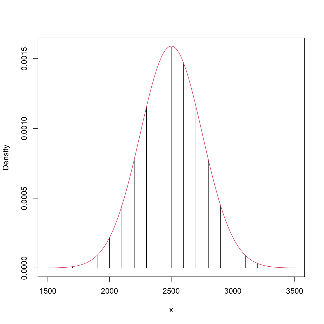

Exercise 6.15 Prove (6.21) for:

Continuous random variables.
Random variables.

Exercise 6.16 Derive (6.20) and, using it, prove that

\[\begin{align*} F_X(x)<F_Y(x)\text{ for all } x\in \mathbb{R}\implies\mathbb{P}[X\geq Y]\geq 0.5. \end{align*}\]

Show that $\mathbb{P}[X\geq Y]>0.5$ is verified if, in addition, $F_X(x)<F_Y(x)$ for $x\in D,$ where $\mathbb{P}[X\in D]>0$ or $\mathbb{P}[Y\in D]>0.$ You can assume $X$ and $Y$ are absolutely continuous variables.

Exercise 6.17 Derive additional counterexamples, significantly different from those in Figures 6.9 and 6.10, for the erroneous claims

$\mu_X>\mu_Y \implies \mathbb{P}[X\geq Y]>0.5;$
$m_X>m_Y \implies \mathbb{P}[X\geq Y]>0.5.$

Exercise 6.18 Verify (6.24) numerically in R with $X$ and $Y$ being continuous random variables. Do so by implementing functions for the test statistics $U_{n,m;\mathrm{MW}}$ and $U_{n,m;\mathrm{W}}.$ Check also that (6.24) is not necessarily satisfied when the samples of $X$ and $Y$ have ties.

6.2.2.2 Wilcoxon signed-rank test

Wilcoxon signed-rank test adapts the Wilcoxon–Mann–Whitney test for paired measurements $(X,Y)$ arising from the same individual.

Test purpose. Given $(X_1,Y_1),\ldots,(X_n,Y_n)\sim F,$ it tests $H_0: F_X=F_Y$ vs. $H_1:\mathbb{P}[X\geq Y]>0.5,$ where $F_X$ and $F_Y$ are the marginal cdfs of $X$ and $Y.$
Statistic definition. Wilcoxon (1945)’s test statistic directly targets $\mathbb{P}[X\geq Y],$²⁵⁵ now using the paired observations, with the (unstandardized) estimator

\[\begin{align} S_n:=\sum_{i=1}^n1_{\{X_i>Y_i\}}.\tag{6.25} \end{align}\]

Values of $S_n$ that are significantly larger than $n/2,$ the expected value under $H_0,$ indicate evidence in favor of $H_1.$
Statistic computation. Computing (6.25) is straightforward.
Distribution under $H_0.$ Under $H_0,$ it follows trivially that $S_n\sim\mathrm{B}(n,0.5).$²⁵⁶
Highlights and caveats. The Wilcoxon signed-rank test shares the same highlights and caveats as its unpaired counterpart. It can be regarded as a “nonparametric paired $t$-test” if both $X$ and $Y$ are symmetric. In this case, it is a nonparametric analogue to the paired $t$-test. Otherwise, it is a nonparametric extension of the paired $t$-test that evaluates if there is a shift in the main mass of probability of $X$ or $Y$ when both are related.²⁵⁷ The test is distribution-free.
Implementation in R. The test statistic $S_n$ and the exact $p$-value are available through the wilcox.test function with paired = TRUE. One must specify alternative = "greater" to test $H_0$ against $H_1:\mathbb{P}[X \boldsymbol{\geq}Y]>0.5.$²⁵⁸ The exact cdf of $S_n$ under $H_0$ is available in psignrank.

The following code exemplifies how to carry out the Wilcoxon signed-rank test.

# Check the test for H0 true
set.seed(123456)
x0 <- rgamma(n = 50, shape = 1, scale = 1)
y0 <- x0 + rnorm(n = 50)
wilcox.test(x = x0, y = y0, paired = TRUE) # H1: P[X >= Y] != 0.5
## 
##  Wilcoxon signed rank test with continuity correction
## 
## data:  x0 and y0
## V = 537, p-value = 0.3344
## alternative hypothesis: true location shift is not equal to 0
wilcox.test(x = x0, y = y0, paired = TRUE, alternative = "greater")
## 
##  Wilcoxon signed rank test with continuity correction
## 
## data:  x0 and y0
## V = 537, p-value = 0.8352
## alternative hypothesis: true location shift is greater than 0
# H1: P[X >= Y] > 0.5
wilcox.test(x = x0, y = y0, paired = TRUE, alternative = "less")
## 
##  Wilcoxon signed rank test with continuity correction
## 
## data:  x0 and y0
## V = 537, p-value = 0.1672
## alternative hypothesis: true location shift is less than 0
# H1: P[X <= Y] > 0.5

# Check the test for H0 false
x1 <- rnorm(n = 50, mean = 0, sd = 1)
y1 <- x1 + rnorm(n = 50, mean = 1, sd = 2)
wilcox.test(x = x1, y = y1, paired = TRUE) # H1: P[X >= Y] != 0.5
## 
##  Wilcoxon signed rank test with continuity correction
## 
## data:  x1 and y1
## V = 255, p-value = 0.0002264
## alternative hypothesis: true location shift is not equal to 0
wilcox.test(x = x1, y = y1, paired = TRUE, alternative = "greater")
## 
##  Wilcoxon signed rank test with continuity correction
## 
## data:  x1 and y1
## V = 255, p-value = 0.9999
## alternative hypothesis: true location shift is greater than 0
# H1: P[X >= Y] > 0.5
wilcox.test(x = x1, y = y1, paired = TRUE, alternative = "less")
## 
##  Wilcoxon signed rank test with continuity correction
## 
## data:  x1 and y1
## V = 255, p-value = 0.0001132
## alternative hypothesis: true location shift is less than 0
# H1: P[X <= Y] > 0.5

Exercise 6.19 Explore by Monte Carlo the power of the following two-sample tests: one-sided Kolmogorov–Smirnov, Wilcoxon–Mann–Whitney, and $t$-test. Take $\delta=$ seq(0, 3, by = 1) as the “deviation strength from $H_0$” for the following scenarios:

$X\sim \mathcal{N}(0.25\delta,1)$ and $Y\sim \mathcal{N}(0,1).$
$X\sim t_3+0.25\delta$ and $Y\sim t_1.$
$X\sim 0.5\mathcal{N}(-\delta,(1 + 0.25 \delta)^2)+0.5\mathcal{N}(\delta,(1 + 0.25 \delta)^2)$ and $Y\sim \mathcal{N}(0,2).$

For each scenario, plot the power curves of the three tests for $n=$ seq(10, 200, by = 10). Use $\alpha=0.05.$ Consider first $M=100$ to have a working solution, then increase it to $M=1,000.$ To visualize all the results effectively, you may want to build a Shiny app that, pre-caching the Monte Carlo study, displays the three power curves with respect to $n,$ for a choice of $\delta,$ scenario, and tests to display. Summarize your conclusions in separated points (you may want to visualize first the models a–b).

6.2.3 Permutation-based approach to comparing distributions

Under the null hypothesis of homogeneity, the iid samples $X_1,\ldots,X_n\sim F$ and $Y_1,\ldots,Y_m\sim G$ have the same distributions. Therefore, since both samples are assumed to be independent from each other,²⁵⁹ they are exchangeable under $H_0:F=G$. This means that, for example, the random vector $(X_1,\ldots,X_{\min(n,m)})^\top$ has the same distribution as $(Y_1,\ldots,Y_{\min(n,m)})^\top$ under $H_0.$ More generally, each of the $p!$ random subvectors of length $p\leq n+m$ that can be extracted without repetitions from $(X_1,\ldots,X_n,Y_1,\ldots,Y_m)^\top$ have the exact same distribution under $H_0.$²⁶⁰ This revelation motivates a resampling procedure that is similar in spirit to the bootstrap seen in Section 6.1.3, yet it is much simpler as it does not require parametric estimation: permutations.

We consider an $N$-permutation function $\sigma:\{1,\ldots,N\}\longrightarrow \{1,\ldots,N\}.$ This function is such that $\sigma(i)=j,$ for certain $i,j\in\{1,\ldots,N\}.$ The number of $N$-permutations quickly becomes extremely large, as there are $N!$ of them.²⁶¹ As an example, if $N=3,$ there exist $3!=6$ possible $3$-permutations $\sigma_1,\ldots,\sigma_6$:

$i$	$\sigma_1(i)$	$\sigma_2(i)$	$\sigma_3(i)$	$\sigma_4(i)$	$\sigma_5(i)$	$\sigma_6(i)$
$1$	$1$	$1$	$2$	$2$	$3$	$3$
$2$	$2$	$3$	$1$	$3$	$1$	$2$
$3$	$3$	$2$	$3$	$1$	$2$	$1$

Using permutations, it is simple to specify that, for any $(n+m)$-permutation $\sigma,$ under $H_0,$

\[\begin{align} (Z_{\sigma(1)},\ldots,Z_{\sigma(n+m)}) \stackrel{d}{=} (Z_1,\ldots,Z_{n+m}), \tag{6.26} \end{align}\]

where we use the standard notation for the pooled sample, $Z_i=X_i$ and $Z_{j+n}=Y_j$ for $i=1,\ldots,n$ and $j=1,\ldots,m.$ A very important consequence of (6.26) is that, under $H_0,$

\[\begin{align*} T_{n,m}(Z_{\sigma(1)},\ldots,Z_{\sigma(n+m)})\stackrel{d}{=}T_{n,m}(Z_1,\ldots,Z_{n+m}) \end{align*}\]

for any proper test statistic $T_{n,m}$ for $H_0:F=G.$ Therefore, denoting $T_{n,m}\equiv T_{n,m}(Z_1,\ldots,Z_{n+m})$ and $T^{\sigma}_{n,m}\equiv T_{n,m}(Z_{\sigma(1)},\ldots,Z_{\sigma(n+m)}),$ it happens that $\mathbb{P}[T_{n,m}\leq x] = \mathbb{P}[T^\sigma_{n,m}\leq x].$ Hence, it readily follows that

\[\begin{align} \mathbb{P}[T_{n,m}\leq x]=\frac{1}{(n+m)!}\sum_{k=1}^{(n+m)!} \mathbb{P}[T^{\sigma_k}_{n,m}\leq x], \tag{6.27} \end{align}\]

where $\sigma_k$ is the $k$-th out of $(n+m)!$ permutations.

We can now exploit (6.27) to approximate the distribution of $T_{n,m}$ under $H_0.$ The key insight is to realize that, conditionally on the observed sample $Z_1,\ldots,Z_{n+m},$ we know whether or not $T^{\sigma_k}_{n,m}\leq x$ is true. We can then replace $\mathbb{P}[T^{\sigma_k}_{n,m}\leq x]$ with its estimation $1_{\big\{T^{\sigma_k}_{n,m}\leq x\big\}}$ in (6.27). However, the evaluation of the sum of $(n+m)!$ terms is often impossible. Instead, an estimation of its value is obtained by considering $B$ randomly-chosen $(n+m)$-permutations of the pooled sample. Joining these two considerations, it follows that

\[\begin{align} \mathbb{P}[T_{n,m}\leq x]\approx \frac{1}{B}\sum_{b=1}^B 1_{\big\{T^{\hat{\sigma}_b}_{n,m}\leq x\big\}}, \tag{6.28} \end{align}\]

where $\hat{\sigma}_b,$ $b=1,\ldots,B,$ denote the $B$ randomly-chosen $(n+m)$-permutations.²⁶²

The null distribution of $T_{n,m}$ can be approximated through (6.28). We summarize next the whole permutation-based procedure for performing a homogeneity test that rejects $H_0$ for large values of the test statistic:

Compute $T_{n,m}\equiv T_{n,m}(Z_1,\ldots,Z_{n+m}).$
Enter the “permutation world”. For $b=1,\ldots,B$:
1. Simulate a randomly-permuted sample $Z_1^{*b},\ldots,Z_{n+m}^{*b}$ from $\{Z_1,\ldots,Z_{n+m}\}.$²⁶³
2. Compute $T_{n,m}^{*b}\equiv T_{n,m}(Z_1^{*b},\ldots,Z_{n+m}^{*b}).$
Obtain the $p$-value approximation

\[\begin{align*} p\text{-value}\approx\frac{1}{B}\sum_{b=1}^B 1_{\{T_{n,m}^{*b}> T_{n,m}\}} \end{align*}\]

and emit a test decision from it. Modify it accordingly if rejection of $H_0$ does not happen for large values of $T_{n,m}.$

The following chunk of code provides a template function for implementing the previous algorithm. It is illustrated with an application of the two-sample Anderson–Darling test to discrete data (using the function ad2_stat).

# A homogeneity test using the Anderson-Darling statistic
perm_comp_test <- function(x, y, B = 1e3, plot_boot = TRUE) {

  # Sizes of x and y
  n <- length(x)
  m <- length(y)

  # Test statistic function. Requires TWO arguments, one being the original
  # data (X_1, ..., X_n, Y_1, ..., Y_m) and the other containing the random
  # index for permuting the sample
  Tn <- function(data, perm_index) {

    # Permute sample by perm_index
    data <- data[perm_index]

    # Split into two samples
    x <- data[1:n]
    y <- data[(n + 1):(n + m)]

    # Test statistic -- MODIFY DEPENDING ON THE PROBLEM
    ad2_stat(x = x, y = y)

  }

  # Perform permutation resampling with the aid of boot::boot
  Tn_star <- boot::boot(data = c(x, y), statistic = Tn,
                        sim = "permutation", R = B)

  # Test information -- MODIFY DEPENDING ON THE PROBLEM
  method <- "Permutation-based Anderson-Darling test of homogeneity"
  alternative <- "any alternative to homogeneity"

  # p-value: modify if rejection does not happen for large values of the
  # test statistic. $t0 is the original statistic and $t has the permuted ones.
  pvalue <- mean(Tn_star$t > Tn_star$t0)

  # Construct an "htest" result
  result <- list(statistic = c("stat" = Tn_star$t0), p.value = pvalue,
                 statistic_perm = drop(Tn_star$t),
                 B = B, alternative = alternative, method = method,
                 data.name = deparse(substitute(x)))
  class(result) <- "htest"

  # Plot the position of the original statistic with respect to the
  # permutation replicates?
  if (plot_boot) {

    hist(result$statistic_perm, probability = TRUE,
         main = paste("p-value:", result$p.value),
         xlab = latex2exp::TeX("$T_{n,m}^*$"))
    rug(result$statistic_perm)
    abline(v = result$statistic, col = 2, lwd = 2)
    text(x = result$statistic, y = 1.5 * mean(par()$usr[3:4]),
         labels = latex2exp::TeX("$T_{n,m}$"), col = 2, pos = 4)

  }

  # Return "htest"
  return(result)

}

# Check the test for H0 true
set.seed(123456)
x0 <- rpois(n = 75, lambda = 5)
y0 <- rpois(n = 75, lambda = 5)
comp0 <- perm_comp_test(x = x0, y = y0, B = 1e3)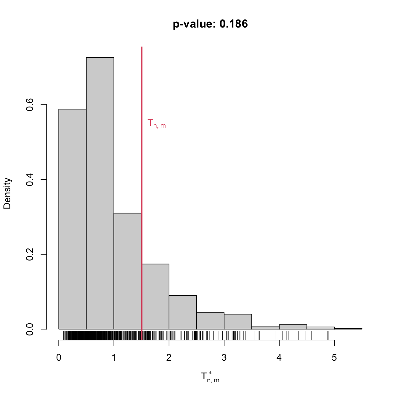

comp0
## 
##  Permutation-based Anderson-Darling test of homogeneity
## 
## data:  x0
## stat = 1.5077, p-value = 0.186
## alternative hypothesis: any alternative to homogeneity

# Check the test for H0 false
x1 <- rpois(n = 50, lambda = 3)
y1 <- rpois(n = 75, lambda = 5)
comp1 <- perm_comp_test(x = x1, y = y1, B = 1e3)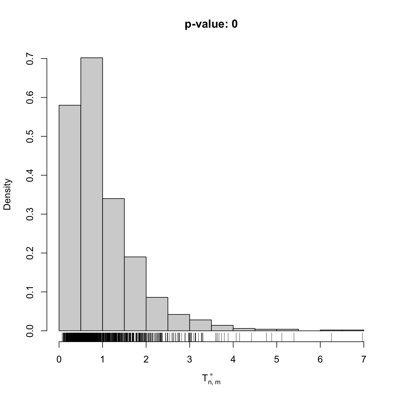

comp1
## 
##  Permutation-based Anderson-Darling test of homogeneity
## 
## data:  x1
## stat = 8.3997, p-value < 2.2e-16
## alternative hypothesis: any alternative to homogeneity

In a paired sample $(X_1,Y_1),\ldots,(X_n,Y_n)\sim F,$ differently to the unpaired case, there is no independence between the $X$- and $Y$-components. Therefore, a variation on the previous permutation algorithm is needed, as the permutation has to be done within the individual observations, and not across individuals. This is achieved by replacing Step i in the previous algorithm with:

Simulate a randomly-permuted sample $(X_1^{*b},Y_1^{*b}),\ldots,(X_n^{*b},Y_n^{*b}),$ where, for each $i=1,\ldots,n,$ $(X_i^{*b},Y_i^{*b})$ is randomly extracted from $\{(X_i,Y_i),(Y_i,X_i)\}.$²⁶⁴

Exercise 6.20 The $F$-statistic $F=\hat{S}^2_1/\hat{S}_2^2$ is employed to test $H_0:\sigma_1^2=\sigma_2^2$ vs. $H_1:\sigma_1^2>\sigma_2^2$ in normal populations $X_1\sim\mathcal{N}(\mu_1,\sigma_1^2)$ and $X_2\sim\mathcal{N}(\mu_2,\sigma_2^2).$ Under $H_0,$ $F$ is distributed as a Snedecor’s $F$ distribution with degrees of freedom $n_1-1$ and $n_2-1.$ The $F$-test is fully parametric. It is implemented in var.test.

The grades.txt dataset contains grades of two exams (e1 and e2) in a certain subject. The group of $41$ students contains two subgroups in mf.

Compute avg, the variable with the average of e1 and e2. Perform a kda of avg for the classes in mf. Are the classes easy to separate? Then, perform a kda for e1 and e2. Are the exams easy to separate?
Compare the variances of avg for each of the subgroups in mf. Which group has larger sample variance? Perform a permutation-based $F$-test to check if the variance of that group is significantly larger. Compare your results with var.test. Are they coherent?
Compare the variances of e1 and e2. Which exam has larger sample variance? Implement a permutation-based paired $F$-test to assess if there are significant differences in the variances. Do it without relying on boot::boot. Compare your results with the unpaired test from part b and with var.test. Are they coherent?

6.3 Independence tests

Assume that a bivariate iid sample $(X_1,Y_1),\ldots,(X_n,Y_n)$ from an arbitrary distribution $F_{X,Y}$ is given. We next address the independence problem of testing the existence of possible dependence between $X$ and $Y.$

Differently to the previous sections, we will approach this problem through the use of coefficients that capture, up to different extension, the degree of dependence between $X$ and $Y.$²⁶⁵ $\!\!^,$²⁶⁶

6.3.1 Concordance-based tests

6.3.1.1 Concordance measures

The random variables $X$ and $Y$ are concordant if “large” values of one tend to be associated with “large” values of the other and, analogously, “small” values of one with “small” values of the other. More precisely, given $(x_i,y_i)$ and $(x_j,y_j),$ two observations of $(X,Y),$ we say that:

$(x_i,y_i)$ and $(x_j,y_j)$ are concordant if $x_i<x_j$ and $y_i<y_j,$ or if $x_i>x_j$ and $y_i>y_j.$
$(x_i,y_i)$ and $(x_j,y_j)$ are discordant if $x_i>x_j$ and $y_i<y_j,$ or if $x_i<x_j$ and $y_i>y_j.$

Alternatively, $(x_i,y_i)$ and $(x_j,y_j)$ are concordant/discordant depending on whether $(x_i-x_j)(y_i-y_j)$ is positive or negative. Therefore, the concordance concept is similar to the correlation concept, but with a main foundational difference: the former does not use the value of $(x_i-x_j)(y_i-y_j),$ only its sign. Consequently, whether $X$ and $Y$ are concordant or discordant will not be driven by its linear association, as happens with positive/negative correlation. One can think about concordance/discordance as a generalized form of positive/negative correlation.

We say that $X$ and $Y$ are concordant/discordant if the “majority” of the observations of $(X,Y)$ are concordant/discordant. This “majority” is quantified by a certain concordance measure. Many concordance measures exist, with different properties and interpretations. Scarsini (1984) gave an axiomatic definition of the properties that any valid concordance measure for continuous random variables must satisfy.

Definition 6.1 (Concordance measure) A measure $\kappa$ of dependence between two continuous random variables $X$ and $Y$ is a concordance measure if it satisfies the following axioms:

Domain: $\kappa(X,Y)$ is defined for any $(X,Y)$ with continuous cdf.
Symmetry: $\kappa(X,Y)=\kappa(Y,X).$
Coherence: $\kappa(X,Y)$ is monotone in $C_{X,Y}$ (the copula of $(X,Y)$).²⁶⁷ That is, if $C_{X,Y}\geq C_{W,Z},$ then $\kappa(X,Y)\geq \kappa(W,Z).$²⁶⁸
Range: $-1\leq\kappa(X,Y)\leq1.$
Independence: $\kappa(X,Y)=0$ if $X$ and $Y$ are independent.
Change of sign: $\kappa(-X,Y)=-\kappa(X,Y).$
Continuity: if $(X,Y)\sim H$ and $(X_n,Y_n)\sim H_n,$ and if $H_n$ converges pointwise to $H$ (and $H_n$ and $H$ continuous), then $\lim_{n\to\infty} \kappa(X_n,Y_n)=\kappa(X,Y).$²⁶⁹

The next theorem, less technical, gives direct insight into what a concordance measure brings on top of correlation: characterize if $(X,Y)$ is such that one variable can be “perfectly predicted” from the other.²⁷⁰ Perfect prediction can only be achieved if each continuous variable is a monotone function $g$ of the other.²⁷¹

Theorem 6.1 Let $\kappa$ be a concordance measure for two continuous random variables $X$ and $Y$:

If $Y=g(X)$ (almost surely) and $g$ is an increasing function, then $\kappa(X,Y)=1.$
If $Y=g(X)$ (almost surely) and $g$ is a decreasing function, then $\kappa(X,Y)=-1.$
If $\alpha$ and $\beta$ are strictly monotonic functions almost everywhere in the supports of $X$ and $Y,$ then $\kappa(\alpha(X),\beta(Y))=\kappa(X,Y).$

Remark. Correlation is not a concordance measure. For example, it fails to verify the third property of Theorem 6.1: $\mathrm{Cor}[X,Y]= \mathrm{Cor}[\alpha(X),\beta(Y)]$ is true only if $\alpha$ and $\beta$ are linear functions.

Important for our interests is Axiom v: independence implies a zero concordance measure, for any proper concordance measure. Note that the converse is false. However, since dependence often manifests itself in concordance patterns, testing independence by testing zero concordance is a useful approach with a more informative rejection of $H_0.$

6.3.1.2 Kendall’s tau and Spearman’s rho

The two most famous measures of concordance for $(X,Y)$ are Kendall’s tau and Spearman’s rho. Both can be regarded as generalizations of $\mathrm{Cor}[X,Y]$ that are not driven by linear relations; rather, they look into the concordance of $(X,Y)$ and the monotone relation between $X$ and $Y.$

The Kendall’s tau of $(X,Y),$ denoted by $\tau(X,Y),$ is defined as

\[\begin{align} \tau(X,Y):=&\,\mathbb{P}[(X-X')(Y-Y')>0]\nonumber\\ &-\mathbb{P}[(X-X')(Y-Y')<0],\tag{6.29} \end{align}\]

where $(X',Y')$ is an iid copy of $(X,Y).$²⁷² $\!\!^,$²⁷³ That is, $\tau(X,Y)$ is the difference of the concordance and discordance probabilities between two random observations of $(X,Y).$

The Spearman’s rho of $(X,Y),$ denoted by $\rho(X,Y),$ is defined as

\[\begin{align} \rho(X,Y):=&\,3\big\{\mathbb{P}[(X-X')(Y-Y'')>0]\nonumber\\ &-\mathbb{P}[(X-X')(Y-Y'')<0]\big\},\tag{6.30} \end{align}\]

where $(X',Y')$ and $(X'',Y'')$ are two iid copies from $(X,Y).$²⁷⁴ Recall that $(X',Y'')$ is a random vector that, by construction, has independent components with marginals equal to those of $(X,Y).$ Hence, $(X',Y'')$ is the “independence version” of $(X,Y)$.²⁷⁵ Therefore, $\rho(X,Y)$ is proportional to the difference of the concordance and discordance probabilities between two random observations, one from $(X,Y)$ and another from its independence version.

A neater interpretation of the Spearman’s rho follows from the following other equivalent definition:

\[\begin{align} \rho(X,Y)=\mathrm{Cor}[F_X(X),F_Y(Y)],\tag{6.31} \end{align}\]

where $F_X$ and $F_Y$ are the marginal cdfs of $X$ and $Y,$ respectively. Expression (6.31) hides the concordance view of $\rho(X,Y),$ but it states that the Spearman’s rho between two random variables is the correlation between their probability transforms.²⁷⁶

Exercise 6.21 Obtain (6.31) from (6.30). Hint: prove first the equality for $X\sim\mathcal{U}(0,1)$ and $Y\sim\mathcal{U}(0,1).$

Although different, Kendall’s tau and Spearman’s rho are heavily related. For example, it is impossible to have $\tau(X,Y)=-0.5$ and $\rho(X,Y)=0.5$ for the same continuous random vector $(X,Y).$ Their relation can be precisely visualized in Figure 6.11, which shows the feasibility region for $(\tau,\rho)$ given by Theorem 6.2. The region is the optimal possible and cannot be narrowed.

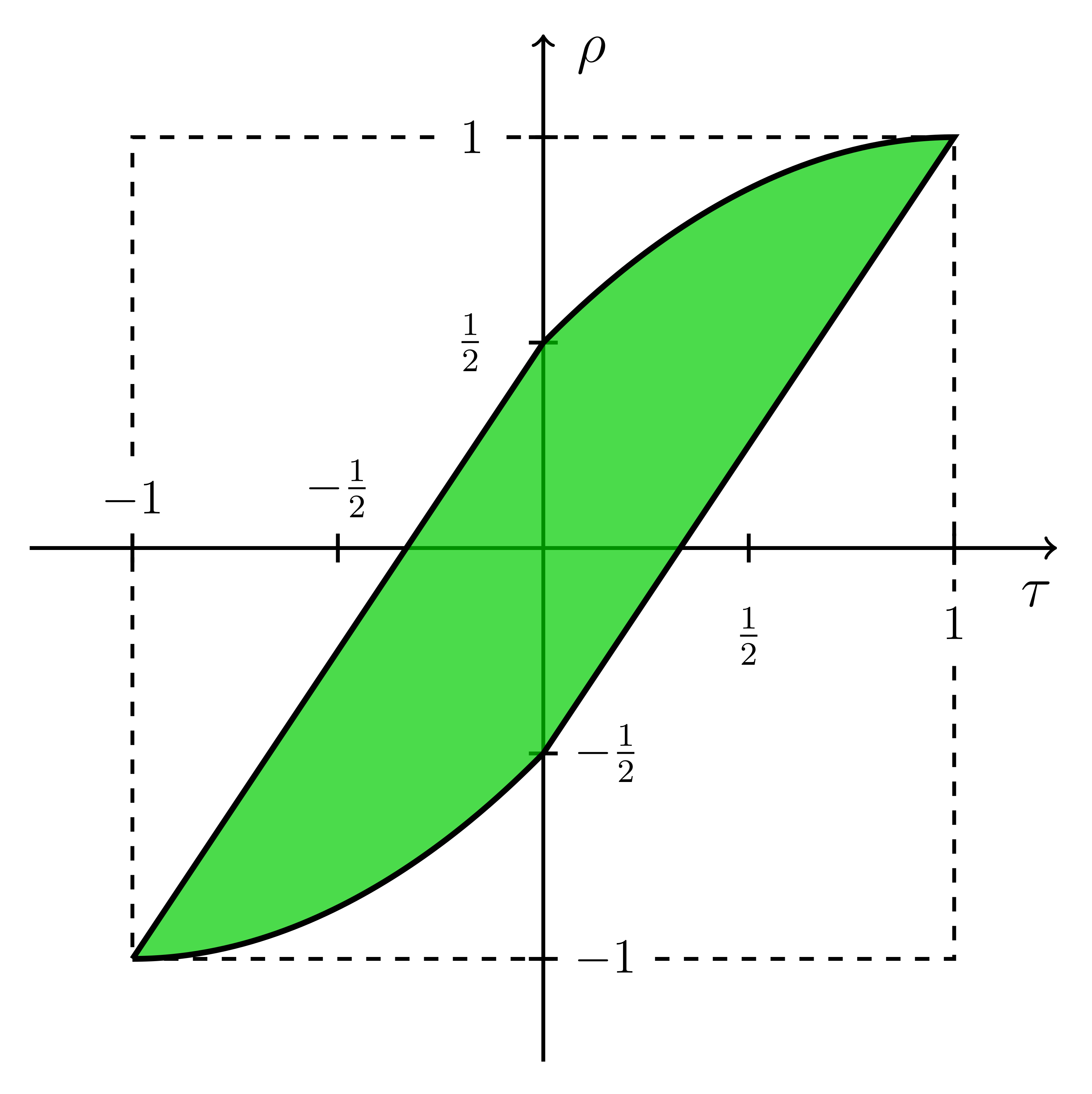
$Feasible region for $(\tau,\rho)$ given by Theorem 6.2.$

Figure 6.11: Feasible region for $(\tau,\rho)$ given by Theorem 6.2.

Theorem 6.2 Let $X$ and $Y$ be two continuous random variables with $\tau\equiv\tau(X,Y)$ and $\rho\equiv\rho(X,Y).$ Then,

\[\begin{align*} \frac{3\tau-1}{2}\leq &\;\rho\leq\frac{1+2\tau-\tau^2}{2},&&\tau\geq 0,\\ \frac{\tau^2+2\tau-1}{2}\leq &\;\rho\leq\frac{1+3\tau}{2},&&\tau\leq 0. \end{align*}\]

6.3.1.3 Kendall’s tau and Spearman’s rho tests of no concordance

Tests purpose. Given $(X_1,Y_1),\ldots,(X_n,Y_n)\sim F_{X,Y},$ test $H_0:\tau=0$ vs. $H_1:\tau\neq0,$ and $H_0:\rho=0$ vs. $H_1:\rho\neq0.$²⁷⁷
Statistics definition. The tests are based on the sample versions of (6.29) and (6.31):

\[\begin{align} \hat\tau:=&\,\frac{c-d}{\binom{n}{2}}=\frac{2(c-d)}{n(n-1)},\tag{6.32}\\ \hat\rho:=&\,\frac{\sum_{i=1}^n(R_i-\bar{R})(S_i-\bar{S})}{\sqrt{\sum_{i=1}^n(R_{i}-\bar{R})^2 \sum_{i=1}^n(S_{i}-\bar{S})^2}},\tag{6.33} \end{align}\]

where $c=\sum_{\substack{i,j=1\\i<j}}^n 1_{\{(X_i-X_j)(Y_i-Y_j)>0\}}$ denotes the number of concordant pairs in the sample, $d=\binom{n}{2}-c$ is the number of discordant pairs, and $R_i:=\mathrm{rank}_X(X_i)=nF_{X,n}(X_i)$ and $S_i:=\mathrm{rank}_Y(Y_i)=nF_{Y,n}(Y_i),$ $i=1,\ldots,n$ are the ranks of the samples of $X$ and $Y.$

Large positive (negative) values of $\hat\tau$ and $\hat\rho$ indicate presence of concordance (discordance) between $X$ and $Y.$ The two-sided tests reject $H_0$ for large absolute values of $\hat\tau$ and $\hat\rho.$
Statistics computation. Formulae (6.32) and (6.33) are reasonably explicit, but the latter can be improved to

\[\begin{align*} \hat\rho=1-\frac{6}{n(n^2-1)}\sum_{i=1}^n(R_i-S_i)^2. \end{align*}\]

The naive computation of $\hat\tau$ involves $O(n^2)$ operations, hence it escalates to large sample sizes worse than $\hat\rho.$ A faster implementation of $O(n\log(n))$ is available through pcaPP::cor.fk.
Distributions under $H_0.$ The asymptotic null distributions of $\hat\tau$ and $\hat\rho$ follow from

\[\begin{align*} \sqrt{\frac{9n(n-1)}{2(2n+5)}}\hat{\tau}\stackrel{d}{\longrightarrow}\mathcal{N}(0,1),\quad \sqrt{n-1}\hat{\rho}\stackrel{d}{\longrightarrow}\mathcal{N}(0,1) \end{align*}\]

under $H_0.$ Exact distributions are available for small $n$’s.
Highlights and caveats. Both $\tau=0$ and $\rho=0$ do not characterize independence. Therefore, absence of rejection does not guarantee lack of evidence in favor of dependence. Rejection of $H_0$ does guarantee the existence of significant dependence, in the form of concordance (positive values of $\hat\tau$ and $\hat\rho$) or discordance (negative values). Both tests are distribution-free.
Implementation in R. The test statistics $\hat\tau$ and $\hat\rho$ and the exact/asymptotic $p$-values are available through the cor.test function, specifying method = "kendall" or method = "spearman". The default alternative = "two.sided" carries out the two-sided tests for $H_1:\tau\neq 0$ and $H_1:\rho\neq 0.$ The one-sided alternatives follows with alternative = "greater" ($>0$) and alternative = "less" ($<0$).

The following chunk of code illustrates the use of cor.test. It also gives some examples of the advantages of $\hat\tau$ and $\hat\rho$ over the correlation coefficient.

# Outliers fool correlation, but do not fool concordance
set.seed(123456)
n <- 200
x <- rlnorm(n)
y <- rlnorm(n)
y[n] <- x[n] <- 5e2
cor.test(x, y, method = "pearson") # Close to 1 due to outlier
## 
##  Pearson's product-moment correlation
## 
## data:  x and y
## t = 189.72, df = 198, p-value < 2.2e-16
## alternative hypothesis: true correlation is not equal to 0
## 95 percent confidence interval:
##  0.9963800 0.9979276
## sample estimates:
##       cor 
## 0.9972609
cor.test(x, y, method = "kendall") # Close to 0, as it should
## 
##  Kendall's rank correlation tau
## 
## data:  x and y
## z = -0.89189, p-value = 0.3725
## alternative hypothesis: true tau is not equal to 0
## sample estimates:
##         tau 
## -0.04241206
cor.test(x, y, method = "spearman") # Close to 0, as it should
## 
##  Spearman's rank correlation rho
## 
## data:  x and y
## S = 1419086, p-value = 0.3651
## alternative hypothesis: true rho is not equal to 0
## sample estimates:
##         rho 
## -0.06434111
cor(rank(x), rank(y)) # Spearman's rho
## [1] -0.06434111
plot(x, y, main = "Massive outlier introduces spurious correlation",
     pch = 16)
abline(lm(y ~ x), col = 2, lwd = 2)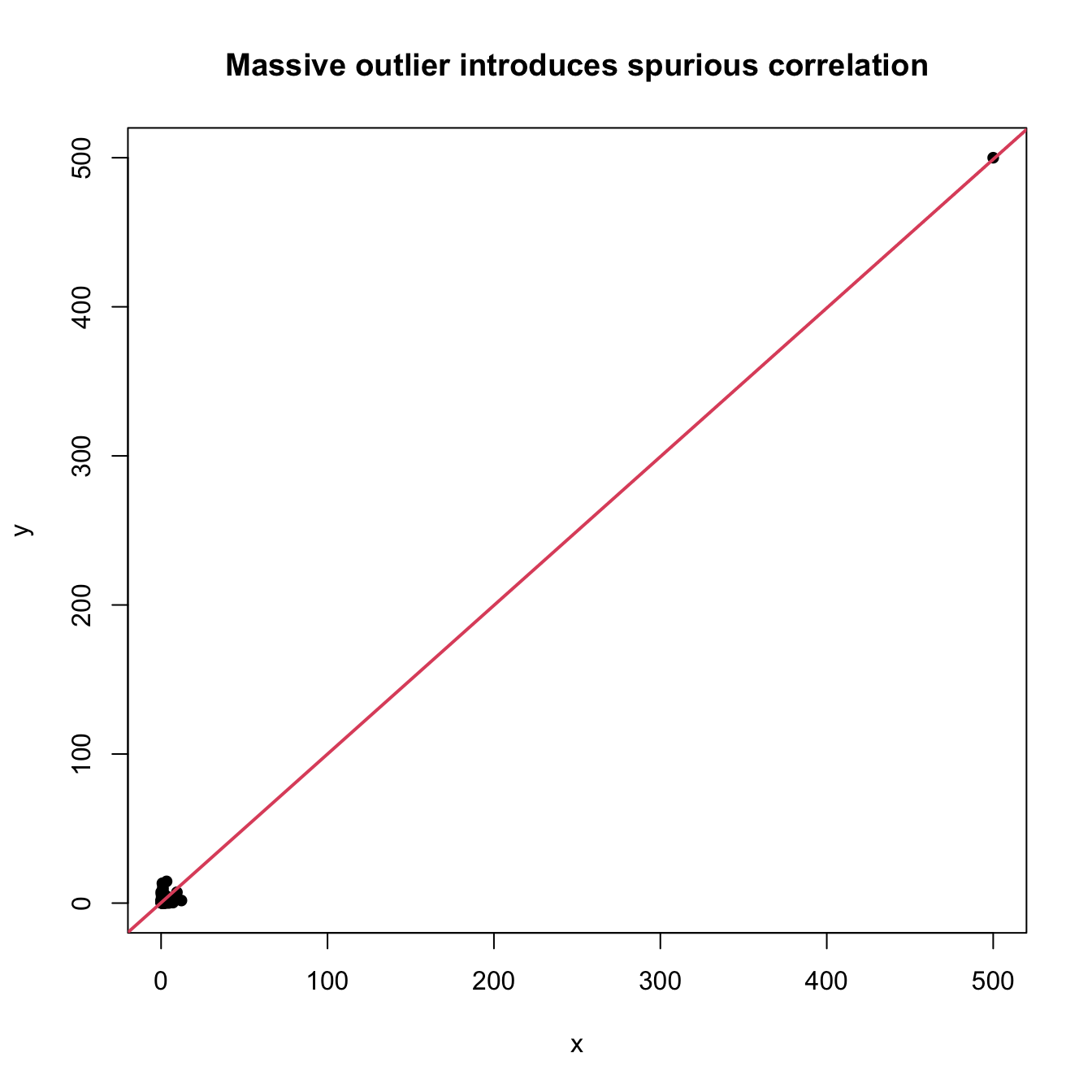

plot(rank(x), rank(y), main = "Concordance is unaffected by outliers",
     pch = 16)
abline(lm(rank(y) ~ rank(x)), col = 2, lwd = 2)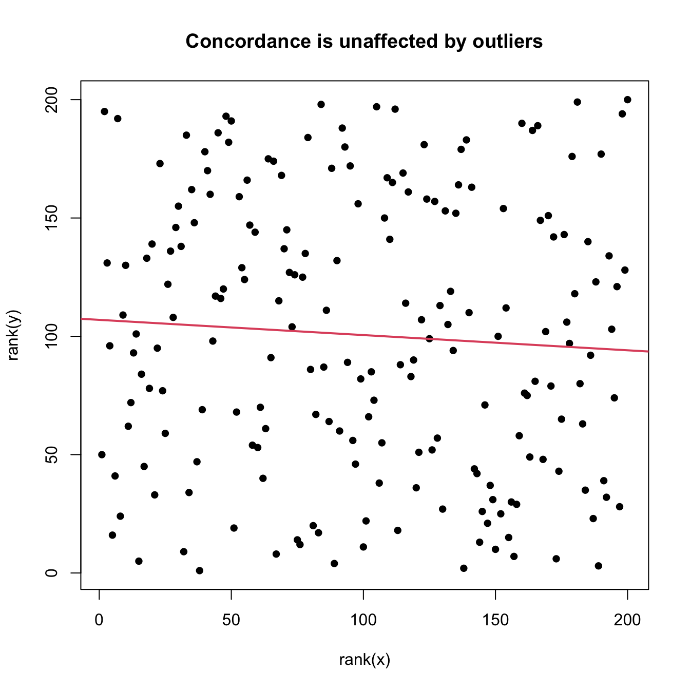


# Outliers fool the sign of correlation, but do not fool concordance
x <- 1000 + rlnorm(n)
y <- x
x[n] <- 1500
y[n] <- 250
cor.test(x, y, method = "pearson", alternative = "greater") # Change of sign!
## 
##  Pearson's product-moment correlation
## 
## data:  x and y
## t = -153.49, df = 198, p-value = 1
## alternative hypothesis: true correlation is greater than 0
## 95 percent confidence interval:
##  -0.9966951  1.0000000
## sample estimates:
##       cor 
## -0.995824
cor.test(x, y, method = "kendall", alternative = "greater") # Fine
## 
##  Kendall's rank correlation tau
## 
## data:  x and y
## z = 20.608, p-value < 2.2e-16
## alternative hypothesis: true tau is greater than 0
## sample estimates:
##  tau 
## 0.98
cor.test(x, y, method = "spearman", alternative = "greater") # Fine
## 
##  Spearman's rank correlation rho
## 
## data:  x and y
## S = 39800, p-value < 2.2e-16
## alternative hypothesis: true rho is greater than 0
## sample estimates:
##       rho 
## 0.9701493
plot(x, y, main = "Massive outlier changes the correlation sign",
     pch = 16)
abline(lm(y ~ x), col = 2, lwd = 2)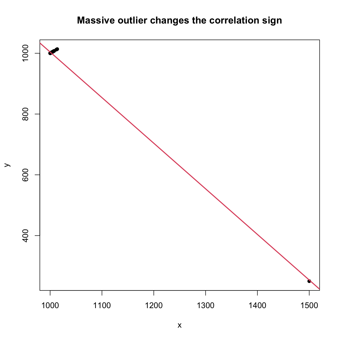

plot(rank(x), rank(y), main = "Concordance is unaffected by outliers",
     pch = 16)
abline(lm(rank(y) ~ rank(x)), col = 2, lwd = 2)

However, as previously said, concordance measures do not characterize independence. Below are some dependence situations that are undetected by $\hat\tau$ and $\hat\rho.$

# Non-monotone dependence fools concordance
set.seed(123456)
n <- 200
x <- rnorm(n)
y <- abs(x) + rnorm(n)
cor.test(x, y, method = "kendall")
## 
##  Kendall's rank correlation tau
## 
## data:  x and y
## z = -1.5344, p-value = 0.1249
## alternative hypothesis: true tau is not equal to 0
## sample estimates:
##         tau 
## -0.07296482
cor.test(x, y, method = "spearman")
## 
##  Spearman's rank correlation rho
## 
## data:  x and y
## S = 1473548, p-value = 0.1381
## alternative hypothesis: true rho is not equal to 0
## sample estimates:
##        rho 
## -0.1051886
plot(x, y, main = "Undetected non-monotone dependence", pch = 16)
abline(lm(y ~ x), col = 2)

plot(rank(x), rank(y), main = "Undetected non-monotone dependence in ranks",
     pch = 16)
abline(lm(rank(y) ~ rank(x)), col = 2, lwd = 2)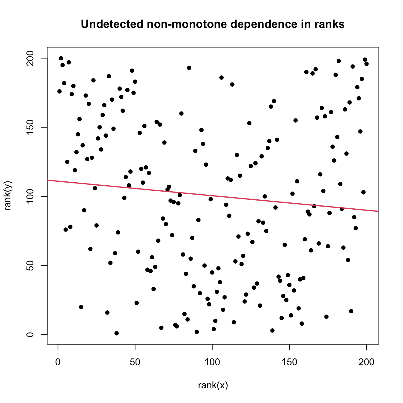


# Dependence in terms of conditional variance fools concordance
x <- rnorm(n)
y <- rnorm(n, sd = abs(x))
cor.test(x, y, method = "kendall")
## 
##  Kendall's rank correlation tau
## 
## data:  x and y
## z = 1.0271, p-value = 0.3044
## alternative hypothesis: true tau is not equal to 0
## sample estimates:
##        tau 
## 0.04884422
cor.test(x, y, method = "spearman")
## 
##  Spearman's rank correlation rho
## 
## data:  x and y
## S = 1251138, p-value = 0.3857
## alternative hypothesis: true rho is not equal to 0
## sample estimates:
##        rho 
## 0.06162304
plot(x, y, main = "Undetected heteroscedasticity", pch = 16)
abline(lm(y ~ x), col = 2)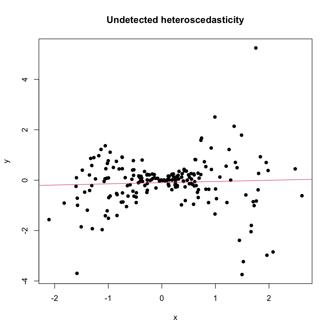

plot(rank(x), rank(y), main = "Undetected heteroscedasticity in ranks",
     pch = 16)
abline(lm(rank(y) ~ rank(x)), col = 2, lwd = 2)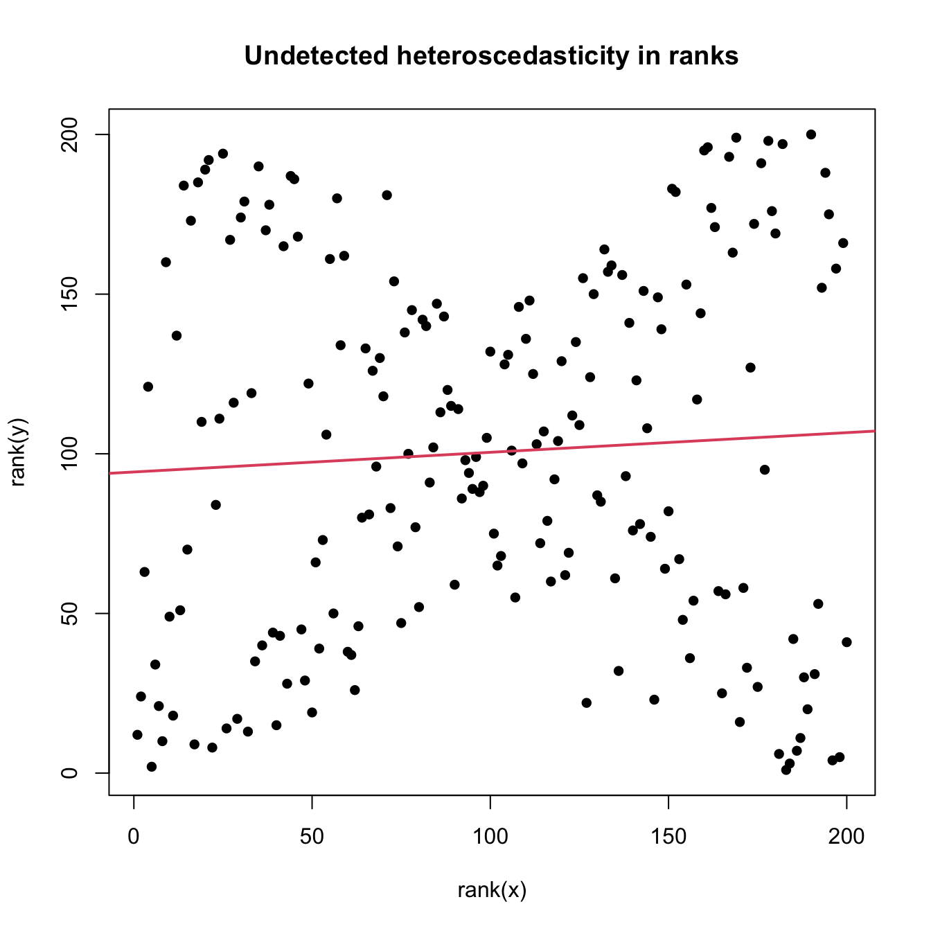

6.3.2 Distance correlation tests

6.3.2.1 A characterization of independence

No-concordance tests based on $\hat\tau$ and $\hat\rho$ are easy to interpret and carry out, but they are not omnibus for testing independence: they do not detect all kinds of dependence between $X$ and $Y,$ only those expressible with $\tau\neq0$ and $\rho\neq0.$ Therefore, and as evidenced previously, Kendall’s tau and Spearman’s rho may not detect dependence patterns in the form of non-monotone relations or heteroscedasticity.

The handicap of concordance measures on not being able to detect all kinds of dependence has been recently solved by Székely, Rizzo, and Bakirov (2007) with the introduction of a new type of correlation measure that completely characterizes independence.²⁷⁸ This new type of correlation is not a correlation between values of $(X,Y).$ Rather, it is related to the correlation between pairwise distances of $X$ and $Y.$ The following definitions, adapted from Section 7.1 in Székely and Rizzo (2017), give the precise form of distance covariance and distance variance between two random variables $X$ and $Y,$ which are the pillars of a distance correlation.

Definition 6.2 (Distance covariance and variance) The distance covariance (dCov) between two random variables $X$ and $Y$ with $\mathbb{E}[|X|]<\infty$ and $\mathbb{E}[|Y|]<\infty$ is the nonnegative number $\mathcal{V}(X,Y)$ with square equal to

\[\begin{align} \mathcal{V}^2(X, Y):=&\,\mathbb{E}\left[|X-X'||Y-Y'|\right]+\mathbb{E}\left[|X-X'|\right] \mathbb{E}\left[|Y-Y'|\right] \nonumber\\ &-2 \mathbb{E}\left[|X-X'||Y-Y''|\right] \tag{6.34}\\ =&\,\mathrm{Cov}\left[|X-X'|,|Y-Y'|\right] \nonumber\\ &- 2\mathrm{Cov}\left[|X-X'|,|Y-Y''|\right],\tag{6.35} \end{align}\]

where $(X',Y')$ and $(X'',Y'')$ are iid copies of $(X,Y).$ The distance variance (dVar) of $X$ is defined as

\[\begin{align} \mathcal{V}^2(X):=&\,\mathcal{V}^2(X, X) \nonumber\\ =&\,\mathbb{V}\mathrm{ar}\left[|X-X'|\right] - 2\mathrm{Cov}\left[|X-X'|,|X-X''|\right].\tag{6.36} \end{align}\]

Some interesting points implicit in Definition 6.2 are:

dCov is unsigned: dCov does not inform on the “direction” of the dependence between $X$ and $Y.$
From (6.34), it is clear that $\mathcal{V}(X, Y)=0$ if $X$ and $Y$ are independent, as in that case $\mathbb{E}\left[|X-X'||Y-Y'|\right] = \mathbb{E}\left[|X-X'|\right]\mathbb{E}\left[|Y-Y'|\right] = \mathbb{E}\left[|X-X'||Y-Y''|\right].$
Equation (6.34) is somehow reminiscent of Spearman’s rho (see (6.30)) and uses $(X',Y''),$ the independence version of $(X,Y).$
As (6.35) points out, dCov is not the covariance between pairwise distances of $X$ and $Y,$ $\mathrm{Cov}\left[|X-X'|,|Y-Y'|\right].$ However, $\mathcal{V}^2(X, Y)$ is related to such covariances: it can be regarded as a covariance between pairwise distances that is “centered” by the covariances of the “independent versions” of the pairwise distances:

\[\begin{align*} \mathcal{V}^2(X, Y)=&\,\mathrm{Cov}\left[|X-X'|,|Y-Y'|\right]\\ &- \mathrm{Cov}\left[|X-X'|,|Y-Y''|\right]- \mathrm{Cov}\left[|X-X''|,|Y-Y'|\right]. \end{align*}\]

Distance correlation is defined analogously to how correlation is defined from covariance and variance.

Definition 6.3 (Distance correlation) The distance correlation (dCor) between two random variables $X$ and $Y$ with $\mathbb{E}[|X|]<\infty$ and $\mathbb{E}[|Y|]<\infty$ is the nonnegative number $\mathcal{R}(X, Y)$ with square equal to

\[\begin{align} \mathcal{R}^2(X, Y):=\frac{\mathcal{V}^2(X, Y)}{\sqrt{\mathcal{V}^2(X) \mathcal{V}^2(Y)}}\tag{6.37} \end{align}\]

if $\mathcal{V}^2(X) \mathcal{V}^2(Y)>0.$ If $\mathcal{V}^2(X) \mathcal{V}^2(Y)=0,$ then $\mathcal{R}^2(X, Y):=0.$

The following theorem collects useful properties of dCov, dVar, and dCor. Some of them are related to the properties of standard covariance (recall, e.g., (1.3)) and (unsigned) correlation. However, as anticipated, Property iv gives the clear edge of dCor over concordance measures on completely characterizing independence.

Theorem 6.3 (Properties of dCov, dVar, and dCor) Let $X$ and $Y$ be two random variables with $\mathbb{E}[|X|]<\infty$ and $\mathbb{E}[|Y|]<\infty.$ Then:

$\mathcal{V}(a+bX, c+dY)=\sqrt{|bd|}\mathcal{V}(X, Y)$ for all $a,b,c,d\in\mathbb{R}.$
$\mathcal{V}(a+bX)=|b|\mathcal{V}(X)$ for all $a,b\in\mathbb{R}.$
If $\mathcal{V}(X)=0,$ then $X=\mathbb{E}[X]$ almost surely.
$\mathcal{R}(X,Y)=\mathcal{V}(X,Y)=0$ if and only if $X$ and $Y$ are independent.
$0\leq \mathcal{R}(X,Y)\leq 1.$
If $\mathcal{R}(X,Y) = 1,$ then there exist $a,b\in\mathbb{R},$ $b\neq0,$ such that $Y = a + bX.$
If $(X,Y)$ is normally distributed and is such that $\mathrm{Cor}[X,Y]=\rho,$ $-1\leq\rho\leq 1,$ then \[\begin{align*} \mathcal{R}^2(X, Y)=\frac{\rho \sin^{-1}(\rho)+\sqrt{1-\rho^2}-\rho \sin^{-1}(\rho/2)-\sqrt{4-\rho^2}+1}{1+\pi / 3-\sqrt{3}} \end{align*}\] and $\mathcal{R}(X, Y)\leq |\rho|.$

$Mapping $\rho\mapsto\mathcal{R}(X(\rho), Y(\rho))$ (in black) for the normally distributed vector $(X(\rho),Y(\rho))$ such that $\mathrm{Cor}\lbrack X(\rho),Y(\rho)\rbrack=\rho.$ In red, the absolute value function $\rho\mapsto|\rho|.$$

Figure 6.12: Mapping $\rho\mapsto\mathcal{R}(X(\rho), Y(\rho))$ (in black) for the normally distributed vector $(X(\rho),Y(\rho))$ such that $\mathrm{Cor}\lbrack X(\rho),Y(\rho)\rbrack=\rho.$ In red, the absolute value function $\rho\mapsto|\rho|.$

Two important simplifications have been done on the previous definitions and theorem for the sake of a simplified exposition. Precisely, dCov admits a more general definition that addresses two generalizations, the first one being especially relevant for practical purposes:

Multivariate extensions. dCov, dVar, and dCor can be straightforwardly extended to account for multivariate vectors $\mathbf{X}$ and $\mathbf{Y}$ supported on $\mathbb{R}^p$ and $\mathbb{R}^q.$ It is as simple as replacing the absolute values $|\cdot|$ in Definition 6.2 with the Euclidean norms $\|\cdot\|_p$ and $\|\cdot\|_q$ for $\mathbb{R}^p$ and $\mathbb{R}^q,$ respectively. The properties stated in Theorem 6.3 hold once suitably adapted. For example, for $\mathbf{X}$ and $\mathbf{Y}$ such that $\mathbb{E}[\|\mathbf{X}\|_p]<\infty$ and $\mathbb{E}[\|\mathbf{Y}\|_q]<\infty,$ dCov is defined as the square root of \[\begin{align*} \mathcal{V}^2(\mathbf{X}, \mathbf{Y}):=&\,\mathrm{Cov}\left[\|\mathbf{X}-\mathbf{X}'\|_p,\|\mathbf{Y}-\mathbf{Y}'\|_q\right]\\ &- 2\mathrm{Cov}\left[\|\mathbf{X}-\mathbf{X}'\|_p,\|\mathbf{Y}-\mathbf{Y}''\|_q\right] \end{align*}\] and dVar as $\mathcal{V}^2(\mathbf{X})=\mathcal{V}^2(\mathbf{X}, \mathbf{X}).$ Recall that both dCov and dVar are scalars, whereas $\mathbb{V}\mathrm{ar}[\mathbf{X}]$ is a $p\times p$ matrix. Consequently, the dCor of $\mathbf{X}$ and $\mathbf{Y}$ is also a scalar that condenses all the dependencies between $\mathbf{X}$ and $\mathbf{Y}.$²⁷⁹
Characteristic-function view of dCov. dCov does not require $\mathbb{E}[|X|]<\infty$ and $\mathbb{E}[|Y|]<\infty$ to be defined. It can be defined, without resorting to expectations, through the characteristic functions²⁸⁰ of $X,$ $Y,$ and $(X,Y)$: \[\begin{align*} \psi_X(s):=\mathbb{E}[e^{\mathrm{i}sX}],\;\, \psi_Y(t):=\mathbb{E}[e^{\mathrm{i}tY}],\;\, \psi_{X,Y}(s,t):=\mathbb{E}[e^{\mathrm{i}(sX+tY)}], \end{align*}\] where $s,t\in\mathbb{R}.$ Indeed, \[\begin{align} \mathcal{V}^2(X,Y)=\frac{1}{c_1^2} \int_{\mathbb{R}^2} \big|\psi_{X,Y}(s, t)-\psi_{X}(s) \psi_{Y}(t)\big|^2\frac{\mathrm{d}t \,\mathrm{d}s}{|t|^2|s|^2},\tag{6.38} \end{align}\] where $c_p:=\pi^{(p+1)/2}/\Gamma((p+1)/2)$ and $|\cdot|$ represents the modulus of a complex number. The alternative definition (6.38) shows that $\mathcal{V}^2(X,Y)$ can be regarded as a weighted squared distance between the joint and marginal characteristic functions, and offers deeper insight into why $\mathcal{V}^2(X,Y)=0$ characterizes independence.²⁸¹ This alternative view also holds for the multivariate case, where (6.38) becomes²⁸² \[\begin{align*} \mathcal{V}^2(\mathbf{X},\mathbf{Y})=\frac{1}{c_pc_q} \int_{\mathbb{R}^p}\int_{\mathbb{R}^q} \big|\psi_{\mathbf{X},\mathbf{Y}}(\mathbf{s}, \mathbf{t})-\psi_{\mathbf{X}}(\mathbf{s}) \psi_{\mathbf{Y}}(\mathbf{t})\big|^2\frac{\mathrm{d}\mathbf{t} \,\mathrm{d}\mathbf{s}}{\|\mathbf{t}\|_q^{q+1}\|\mathbf{s}\|_p^{p+1}}. \end{align*}\]

6.3.2.2 Distance correlation test

Independence tests for $(X,Y)$ can be constructed by evaluating if $\mathcal{R}(X,Y)$ or $\mathcal{V}(X,Y)=0$ holds. To do so, we first need to consider the empirical versions of dCov and dCor. These follow from (6.34) and (6.37).

Definition 6.4 (Empirical distance covariance and variance) The dCov for the random sample $(X_1,Y_1),\ldots,(X_n,Y_n)$ is the nonnegative number $\mathcal{V}_n(X,Y)$ with square equal to

\[\begin{align} \mathcal{V}_n^2(X,Y):=&\,\frac{1}{n^2} \sum_{k, \ell=1}^n A_{k \ell} B_{k \ell},\tag{6.39} \end{align}\]

where

\[\begin{align*} A_{k \ell}:=&\,a_{k \ell}-\bar{a}_{k \bullet}-\bar{a}_{\bullet \ell}+\bar{a}_{\bullet\bullet},\quad a_{k \ell}:=|X_k-X_\ell|,\\ \bar{a}_{k \bullet}:=&\,\frac{1}{n} \sum_{l=1}^n a_{k \ell},\quad \bar{a}_{\bullet \ell}:=\frac{1}{n} \sum_{k=1}^n a_{k \ell},\quad \bar{a}_{\bullet \bullet}:=\frac{1}{n^2} \sum_{k, \ell=1}^n a_{k \ell}, \end{align*}\]

and $B_{k \ell}:=b_{k \ell}-\bar{b}_{k \bullet}-\bar{b}_{\bullet \ell}+\bar{b}_{\bullet\bullet}$ is defined analogously for $b_{k \ell}:=|Y_k-Y_\ell|.$ The dVar of $X_1,\ldots,X_n$ is defined as $\mathcal{V}_n^2(X):=\frac{1}{n^2} \sum_{k, \ell=1}^n A_{k \ell}^2.$

Definition 6.5 (Empirical distance correlation) The dCor for the random sample $(X_1,Y_1),\ldots,(X_n,Y_n)$ is the nonnegative number $\mathcal{R}_n(X, Y)$ with square equal to

\[\begin{align} \mathcal{R}_n^2(X, Y):=\frac{\mathcal{V}_n^2(X, Y)}{\sqrt{\mathcal{V}_n^2(X) \mathcal{V}_n^2(Y)}}\tag{6.40} \end{align}\]

if $\mathcal{V}_n^2(X) \mathcal{V}_n^2(Y)>0.$ If $\mathcal{V}_n^2(X) \mathcal{V}_n^2(Y)=0,$ then $\mathcal{R}_n^2(X, Y):=0.$

Remark. The previous empirical versions of dCov, dVar, and dCor also allow for multivariate versions. These are based on $a_{k \ell}:=\|\mathbf{X}_k-\mathbf{X}_\ell\|_p$ and $b_{k \ell}:=\|\mathbf{Y}_k-\mathbf{Y}_\ell\|_q.$

We next introduce the independence tests based on (6.39)–(6.40).

Test purpose. Given $(X_1,Y_1),\ldots,(X_n,Y_n)\sim F_{X,Y},$ test $H_0:F_{X,Y}=F_XF_Y$ vs. $H_1:F_{X,Y}\neq F_XF_Y$ consistently against all the alternatives in $H_1.$
Statistic definition. The dCov test rejects $H_0$ for large values of the test statistic $n\mathcal{V}_n^2(X,Y)$ (not the dCov!), which indicates a departure from independence. The dCor test uses as test statistic $\mathcal{R}_n^2(X,Y)$ and rejects $H_0$ for large values of it.
Statistic computation. Formulae (6.39) and (6.40) are directly implementable, yet they involve $O(n^2)$ computations.²⁸³
Distribution under $H_0.$ If $H_0$ holds, then the asymptotic cdf of $n\mathcal{V}_n^2(X,Y)$ is the cdf of the random variable

\[\begin{align} \sum_{j=1}^\infty\lambda_j Y_j,\quad \text{where } Y_j\sim\chi^2_1,\,j\geq 1,\text{ are iid}\tag{6.41} \end{align}\]

and $\{\lambda_j\}_{j=1}^\infty$ are certain nonnegative constants that depend on $F_{X,Y}$ (so the test is not distribution-free). As with (6.8), the cdf of (6.41) does not admit a simple analytical expression. In addition, it is mostly unusable in practice, since $\{\lambda_j\}_{j=1}^\infty$ are unknown. The asymptotic distribution for $\mathcal{R}_n^2(X,Y)$ is related to that of $n\mathcal{V}_n^2(X,Y).$ However, both test statistics can be calibrated by permutations (see Section 6.3.3).
Highlights and caveats. On the positive side, the dCov/dCor test is much more general than concordance-based tests: (i) it is an omnibus test for independence; and (ii) it can be applied to multivariate data. On the negative side, the dCov/dCor test is not distribution-free, so fast asymptotic $p$-values are not available. Besides, the rejection of the dCov/dCor tests does not inform on the kind of dependence between $X$ and $Y.$ The dCov and dCor tests perform similarly and their computational burdens are roughly equivalent. The dCor test offers the edge of having an absolute scale for its test statistic, since $\mathcal{R}_n^2(X,Y)\in[0,1].$
Implementation in R. The energy package implements both tests through the energy::dcov.test and energy::dcor.test functions, which compute the test statistics and give $p$-values approximated by permutations (see Section 6.3.3).

The use of energy::dcov.test and energy::dcor.test for testing the independence between $X$ and $Y$ is shown in the following chunk of code.

# Distance correlation detects non-monotone dependence
set.seed(123456)
n <- 200
x <- rnorm(n)
y <- abs(x) + rnorm(n)

# Distance covariance and correlation tests. R is the number of permutations
# and needs to be specified (the default is R = 0 -- no test is produced)
energy::dcov.test(x, y, R = 1e3)
## 
##  dCov independence test (permutation test)
## 
## data:  index 1, replicates 1000
## nV^2 = 6.4595, p-value = 0.001998
## sample estimates:
##      dCov 
## 0.1797145
energy::dcor.test(x, y, R = 1e3)
## 
##  dCor independence test (permutation test)
## 
## data:  index 1, replicates 1000
## dCor = 0.26188, p-value = 0.000999
## sample estimates:
##      dCov      dCor   dVar(X)   dVar(Y) 
## 0.1797145 0.2618840 0.6396844 0.7361771

# Distance correlation detects conditional variance as dependence
x <- rnorm(n)
y <- rnorm(n, sd = abs(x))

# Distance covariance and correlation tests
energy::dcov.test(x, y, R = 1e3)
## 
##  dCov independence test (permutation test)
## 
## data:  index 1, replicates 1000
## nV^2 = 3.5607, p-value = 0.001998
## sample estimates:
##      dCov 
## 0.1334296
energy::dcor.test(x, y, R = 1e3)
## 
##  dCor independence test (permutation test)
## 
## data:  index 1, replicates 1000
## dCor = 0.25031, p-value = 0.004995
## sample estimates:
##      dCov      dCor   dVar(X)   dVar(Y) 
## 0.1334296 0.2503077 0.6152985 0.4618172

Testing the independence of two random vectors $\mathbf{X}$ and $\mathbf{Y}$ is also straightforward, as the code below illustrates.

# A multivariate case with independence
set.seed(123456)
n <- 200
p <- 5
x <- matrix(rnorm(n * p), nrow = n, ncol = p)
y <- matrix(rnorm(n * p), nrow = n, ncol = p)
energy::dcov.test(x, y, R = 1e3)
## 
##  dCov independence test (permutation test)
## 
## data:  index 1, replicates 1000
## nV^2 = 8.5627, p-value = 0.7493
## sample estimates:
##      dCov 
## 0.2069139
energy::dcor.test(x, y, R = 1e3)
## 
##  dCor independence test (permutation test)
## 
## data:  index 1, replicates 1000
## dCor = 0.28323, p-value = 0.7732
## sample estimates:
##      dCov      dCor   dVar(X)   dVar(Y) 
## 0.2069139 0.2832256 0.7163536 0.7450528

# A multivariate case with dependence
y <- matrix(0.2 * rnorm(n = n * p, mean = c(x)) +
              rnorm(n * p, sd = 1.25), nrow = n, ncol = p)
energy::dcov.test(x, y, R = 1e3)
## 
##  dCov independence test (permutation test)
## 
## data:  index 1, replicates 1000
## nV^2 = 14.592, p-value = 0.01099
## sample estimates:
##      dCov 
## 0.2701076
energy::dcor.test(x, y, R = 1e3)
## 
##  dCor independence test (permutation test)
## 
## data:  index 1, replicates 1000
## dCor = 0.32299, p-value = 0.007992
## sample estimates:
##      dCov      dCor   dVar(X)   dVar(Y) 
## 0.2701076 0.3229851 0.7163536 0.9762951

Exercise 6.22 Illustrate with a simulation study the performance of the independence tests for $(X,Y)$ based on Pearson’s correlation, Spearman’s rho, and distance covariance. To that end, use five simulation scenarios and build a $5\times 4$ plot such that:

The first column contains illustrative scatterplots of the generated data.
The second, third, and fourth column show histograms of the $p$-values of Pearson’s correlation, Spearman’s rho, and distance covariance tests in that scenario, respectively.

For the four scenarios, consider: (1) independence; (2) an alternative where Pearson’s correlation test has the largest power; (3) an alternative where Spearman’s rho has the largest power; (4) an alternative for which all tests have similar powers; (5) an undetectable alternative by Spearman’s rho. Choose the scenarios originally and in such a way the histograms of the $p$-values are not completely extreme. Use $M=1,000$ Monte Carlo replicates and set $n=100.$ Use permutations to obtain the $p$-values in all tests for a fairer comparison, setting $B=500.$ Explain the obtained results.

6.3.3 Permutation-based approach to testing independence

The calibration of a test of independence can be approached by permutations, in an analogous way as that carried out in Section 6.2.3 for tests of homogeneity. None of the permutation strategies previously seen is adequate, though, since the independence problem, expressed as

\[\begin{align*} H_0:F_{X,Y}=F_XF_Y\quad\text{vs.}\quad H_1:F_{X,Y}\neq F_XF_Y, \end{align*}\]

is substantially different from (6.13). Here, $F_{X,Y}$ represents the joint cdf of $(X,Y),$ $F_X$ and $F_Y$ stand for the corresponding marginal cdfs, and “$F_{X,Y}\neq F_XF_Y$” denotes that there exists at least one $(x,y)\in\mathbb{R}^2$ such that $F_{X,Y}(x,y)\neq F_X(x)F_Y(y).$

In the unpaired homogeneity case, the elements of the samples $X_1,\ldots,X_n$ and $Y_1,\ldots,Y_m$ are randomly exchanged using the pooled sample. In the paired case, the components of each pair $(X_1,Y_1),\ldots,(X_n,Y_n)$ are randomly exchanged. When testing for independence, each of the two sample components of $(X_1,Y_1),\ldots,(X_n,Y_n)$ are separately and randomly exchanged. That the resampling is conducted separately for each component is a direct consequence of the null hypothesis of independence.

Precisely, for any two $n$-permutations $\sigma_1$ and $\sigma_2,$ under independence, it happens that

\[\begin{align*} T_n((X_{\sigma_1(1)},Y_{\sigma_2(1)}),\ldots,(X_{\sigma_1(n)},Y_{\sigma_2(n)}))\stackrel{d}{=}T_n((X_1,Y_1),\ldots,(X_n,Y_n)) \end{align*}\]

for any proper independence test statistic $T_n.$ Furthermore, it is reasonably evident that

\[\begin{align*} T_n((X_{\sigma_1(1)},Y_{\sigma_2(1)}),\ldots,(X_{\sigma_1(n)},Y_{\sigma_2(n)}))=T_n((X_1,Y_{\sigma_3(1)}),\ldots,(X_n,Y_{\sigma_3(n)})) \end{align*}\]

for $\sigma_3(i):=\sigma_2(\sigma_1^{-1}(i)),$ $i\in\{1,\ldots,n\}.$²⁸⁴ That is, any “double permutation” amounts to “single permutation” and it suffices to permute the second component of the sample (leaving the first component fixed) to attain any of the possible values of $T_n((X_{\sigma_1(1)},Y_{\sigma_2(1)}),\ldots,(X_{\sigma_1(n)},Y_{\sigma_2(n)})).$ From the previous arguments, it follows that

\[\begin{align*} \mathbb{P}[T_n\leq x]=\frac{1}{n!}\sum_{k=1}^{n!} \mathbb{P}[T^{\sigma_k}_n\leq x]\approx \frac{1}{B}\sum_{b=1}^{B} 1_{\big\{T^{\hat{\sigma}_b}_n\leq x\big\}}, \end{align*}\]

where $T^{\sigma}_n\equiv T_n((X_1,Y_{\sigma(1)}),\ldots,(X_n,Y_{\sigma(n)}))$ and $\hat{\sigma}_b,$ $b=1,\ldots,B,$ denote the $B$ randomly-chosen $n$-permutations.

The whole permutation-based procedure for performing an independence test that rejects $H_0$ for large values of the test statistic is summarized below:

Compute $T_n\equiv T_n((X_1,Y_1),\ldots,(X_n,Y_n)).$
Enter the “permutation world”. For $b=1,\ldots,B$:
1. Simulate a randomly-permuted sample $Y_1^{*b},\ldots,Y_n^{*b}$ from $\{Y_1,\ldots,Y_n\}.$²⁸⁵
2. Compute $T_n^{*b}\equiv T_n((X_1,Y_1^{*b}),\ldots,(X_n,Y_n^{*b})).$
Obtain the $p$-value approximation

\[\begin{align*} p\text{-value}\approx\frac{1}{B}\sum_{b=1}^B 1_{\{T_n^{*b}> T_n\}} \end{align*}\]

and emit a test decision from it. Modify it accordingly if rejection of $H_0$ does not happen for large values of $T_n.$

The following chunk of code provides a template for implementing the previous permutation algorithm.

# A no-association test using the absolute value of Spearman's rho statistic
perm_ind_test <- function(x, B = 1e3, plot_boot = TRUE) {

  # Test statistic function. Requires TWO arguments, one being the original
  # data (X_1, Y_1), ..., (X_n, Y_n) and the other containing the random
  # index for permuting the second component of sample
  Tn <- function(data, perm_index) {

    # Permute sample by perm_index -- only permute the second component
    data[, 2] <- data[, 2][perm_index]

    # Test statistic -- MODIFY DEPENDING ON THE PROBLEM
    abs(cor(x = data[, 1], y = data[, 2], method = "spearman"))

  }

  # Perform permutation resampling with the aid of boot::boot
  Tn_star <- boot::boot(data = x, statistic = Tn, sim = "permutation", R = B)

  # Test information -- MODIFY DEPENDING ON THE PROBLEM
  method <- "Permutation-based Spearman's rho test of no concordance"
  alternative <- "Spearman's rho is not zero"

  # p-value: modify if rejection does not happen for large values of the
  # test statistic. $t0 is the original statistic and $t has the permuted ones.
  pvalue <- mean(Tn_star$t > Tn_star$t0)

  # Construct an "htest" result
  result <- list(statistic = c("stat" = Tn_star$t0), p.value = pvalue,
                 statistic_perm = drop(Tn_star$t),
                 B = B, alternative = alternative, method = method,
                 data.name = deparse(substitute(x)))
  class(result) <- "htest"

  # Plot the position of the original statistic with respect to the
  # permutation replicates?
  if (plot_boot) {

    hist(result$statistic_perm, probability = TRUE,
         main = paste("p-value:", result$p.value),
         xlab = latex2exp::TeX("$T_n^*$"))
    rug(result$statistic_perm)
    abline(v = result$statistic, col = 2, lwd = 2)
    text(x = result$statistic, y = 1.5 * mean(par()$usr[3:4]),
         labels = latex2exp::TeX("$T_n$"), col = 2, pos = 4)

  }

  # Return "htest"
  return(result)

}

# Check the test for H0 true
set.seed(123456)
x0 <- mvtnorm::rmvnorm(n = 100, mean = c(0, 0), sigma = diag(c(1:2)))
ind0 <- perm_ind_test(x = x0, B = 1e3)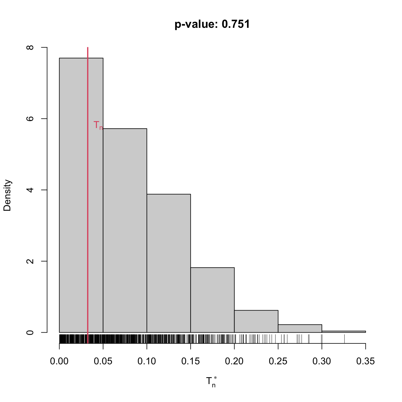

ind0
## 
##  Permutation-based Spearman's rho test of no concordance
## 
## data:  x0
## stat = 0.032439, p-value = 0.751
## alternative hypothesis: Spearman's rho is not zero

# Check the test for H0 false
x1 <- mvtnorm::rmvnorm(n = 100, mean = c(0, 0), sigma = toeplitz(c(1, 0.5)))
ind1 <- perm_ind_test(x = x1, B = 1e3)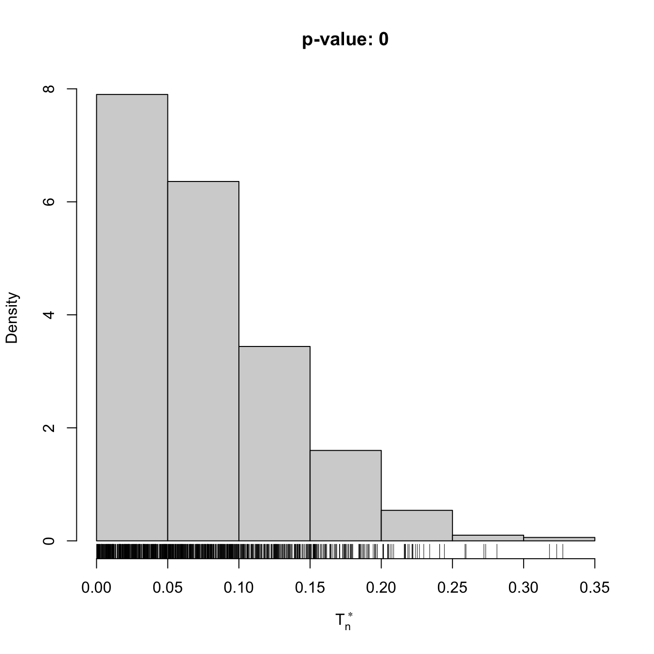

ind1
## 
##  Permutation-based Spearman's rho test of no concordance
## 
## data:  x1
## stat = 0.52798, p-value < 2.2e-16
## alternative hypothesis: Spearman's rho is not zero

References

Anderson, T. W. 1962. “On the Distribution of the Two-Sample Cramer-von Mises Criterion.” The Annals of Mathematical Statistics 33 (3): 1148–59. https://doi.org/10.1214/aoms/1177704477.

Barrio, E. del. 2007. “Empirical and Quantile Processes in the Asymptotic Theory of Goodness-of-Fit Tests.” In Lectures on Empirical Processes, 1–92. EMS Series of Lectures in Mathematics. Zürich: European Mathematical Society. https://doi.org/10.4171/027.

Blum, J. R., J. Kiefer, and M. Rosenblatt. 1961. “Distribution Free Tests of Independence Based on the Sample Distribution Function.” The Annals of Mathematical Statistics 32 (2): 485–98. https://doi.org/10.1214/aoms/1177705055.

D’Agostino, R. B., and M. A. Stephens, eds. 1986. Goodness-of-Fit Techniques. Vol. 68. Statistics: Textbooks and Monographs. New York: Marcel Dekker. https://www.routledge.com/Goodness-of-Fit-Techniques/DAgostino/p/book/9780367580346.

Dallal, G. E., and L. Wilkinson. 1986. “An Analytic Approximation to the Distribution of Lilliefors’s Test Statistic for Normality.” The American Statistician 40 (4): 294–96. https://doi.org/10.1080/00031305.1986.10475419.

González-Manteiga, W., and R. M. Crujeiras. 2013. “An Updated Review of Goodness-of-Fit Tests for Regression Models.” TEST 22 (3): 361–411. https://doi.org/10.1007/s11749-013-0327-5.

Lilliefors, H. W. 1967. “On the Kolmogorov-Smirnov Test for Normality with Mean and Variance Unknown.” Journal of the American Statistical Association 62 (318): 399–402. https://doi.org/10.1080/01621459.1967.10482916.

Mann, H. B., and D. R. Whitney. 1947. “On a Test of Whether One of Two Random Variables Is Stochastically Larger Than the Other.” The Annals of Mathematical Statistics 18 (1): 50–60. https://doi.org/10.1214/aoms/1177730491.

Molina Peralta, I., and E. García-Portugués. 2025. A First Course on Statistical Inference. https://egarpor.github.io/SI-UC3M/.

Pettitt, A. N. 1976. “A Two-Sample Anderson-Darling Rank Statistic.” Biometrika 63 (1): 161–68. https://doi.org/10.1093/biomet/63.1.161.

Rizzo, M. L., and G. J. Székely. 2016. “Energy Distance.” WIREs Computational Statistics 8 (1): 27–38. https://doi.org/10.1002/wics.1375.

Royston, P. 1993. “A Pocket-Calculator Algorithm for the Shapiro-Francia Test for Non-Normality: An Application to Medicine.” Statistics in Medicine 12 (2): 181–84. https://doi.org/10.1002/sim.4780120209.

Scarsini, M. 1984. “On Measures of Concordance.” Stochastica 8: 201–18. https://dmle.icmat.es/revistas/detalle.php?numero=1689.

Shao, J. 1999. Mathematical Statistics. Springer Texts in Statistics. New York: Springer. https://doi.org/10.1007/b97553.

Stephens, M. A. 1974. “EDF Statistics for Goodness of Fit and Some Comparisons.” Journal of the American Statistical Association 69 (347): 730–37. https://doi.org/10.2307/2286009.

Székely, G. J., and M. L. Rizzo. 2013. “Energy Statistics: A Class of Statistics Based on Distances.” Journal of Statistical Planning and Inference 143 (8): 1249–72. https://doi.org/10.1016/j.jspi.2013.03.018.

———. 2017. “The Energy of Data.” Annual Review of Statistics and Its Application 4 (1): 447–79. https://doi.org/10.1146/annurev-statistics-060116-054026.

Székely, G. J., M. L. Rizzo, and N. K. Bakirov. 2007. “Measuring and Testing Dependence by Correlation of Distances.” The Annals of Statistics 35 (6): 2769–94. https://doi.org/10.1214/009053607000000505.

Velilla, S. 1994. “A Goodness-of-Fit Test for Autoregressive Moving-Average Models Based on the Standardized Sample Spectral Distribution of the Residuals.” Journal of Time Series Analysis 15 (6): 637–47. https://doi.org/10.1111/j.1467-9892.1994.tb00218.x.

Wilcoxon, F. 1945. “Individual Comparisons by Ranking Methods.” Biometrics Bulletin 1 (6): 80–83. https://doi.org/10.2307/3001968.

If necessary, see Section C for an informal review on the main concepts involved in hypothesis testing.↩︎
This prior assessment is of key importance to ensure coherency between the real and the assumed data distributions, as the parametric test bases its decision on the latter. An example to dramatize this point follows. Let $X_1\sim\mathcal{N}(\mu,\sigma^2)$ and $X_2\sim\Gamma(\mu/\sigma^2,\mu^2/\sigma^2),$ for $\mu,\sigma^2>0.$ The cdfs of $X_1$ and $X_2,$ $F_1$ and $F_2,$ are different for all $\mu,\sigma^2>0.$ Yet $\mathbb{E}[X_1]=\mathbb{E}[X_2]$ and $\mathbb{V}\mathrm{ar}[X_1]=\mathbb{V}\mathrm{ar}[X_2].$ When testing $H_0:F_1=F_2,$ if one assumes that $X_1$ and $X_2$ are normally distributed (which is partially true), then one can use a $t$-test with unknown variances. The $t$-test will believe $H_0$ is true, since $\mathbb{E}[X_1]=\mathbb{E}[X_2]$ and $\mathbb{V}\mathrm{ar}[X_1]=\mathbb{V}\mathrm{ar}[X_2],$ thus having a rejection rate equal to the significance level $\alpha.$ However, by construction, $H_0$ is false. The $t$-test fails to reject $H_0$ because its parametric assumption does not match the reality.↩︎
These optimal parametric tests are often obtained by maximum likelihood theory.↩︎
See, e.g., Section 6.2 in Molina Peralta and García-Portugués (2025).↩︎
See González-Manteiga and Crujeiras (2013) for an exhaustive review of the topic.↩︎
For example, there are goodness-of-fit tests for time series models, such as $\mathrm{ARMA}(p,q)$ models (see, e.g., Velilla (1994) and references therein).↩︎
$F$ does not need to be continuous.↩︎
The fact that $F=F_0$ is tested in full generality against any distribution that is different from $F_0$ raises the omnibus test (all-purpose test) terminology for the kind of tests that are able to detect all the alternatives to $H_0$ that are within $H_1.$↩︎
That is, the tests will have a rejection probability lower than $\alpha$ when $H_0$ is true.↩︎
If $F$ and $F_0$ were continuous, the density approach to this problem would compare the kde $\hat{f}(\cdot;h)$ seen in Chapter 2 with the density $f_0.$ While using a kde for testing $H_0:F=F_0$ via $H_0:f=f_0$ is a perfectly valid approach and has certain advantages (e.g., better detection of local violations of $H_0$), it is also more demanding (it requires selecting the bandwidth $h$) and limited (applicable to continuous random variables only). The cdf optic, although not appropriate for visualization or for the applications described in Section 3.5, suffices for conducting hypothesis testing in a nonparametric way.↩︎
A popular approach to goodness-of-fit tests, not covered in this book, is the chi-squared test (see ?chisq.test). This test is based on aggregating the values of $X$ in $k$ classes $I_i,$ $i=1,\ldots,k,$ where $\cup_{i=1}^k I_i$ cover the support of $X.$ Worryingly, one can modify the outcome of the test by altering the form of these classes and the choice of $k$ – a sort of tuning parameter. The choice of $k$ also affects the quality of the asymptotic null distribution. Therefore, for continuous and discrete random variables, the chi-squared test has significant drawbacks when compared to the ecdf-based tests. Nevertheless, the “chi-squared philosophy” of testing is remarkably general: as opposed to ecdf-based tests, it can be readily applied to the analysis of categorical variables and contingency tables.↩︎
Or the $\infty$-distance $\|F_n-F_0\|_\infty=\sup_{x\in\mathbb{R}} \left|F_n(x)-F_0(x)\right|.$↩︎
With the addition of the $\sqrt{n}$ factor in order to standardize $D_n$ in terms of its asymptotic distribution under $H_0.$ Many authors do not consider this factor as a part of the test statistic itself.↩︎
Notice that $F_n(X_{(i)})=\frac{i}{n}$ and $F_n(X_{(i)}^-)=\frac{i-1}{n}.$↩︎
When the sample size $n$ is large: $n\to\infty.$↩︎
The infinite series converges quite fast and $50$ terms are usually enough to evaluate (6.3) with high accuracy for $x\in\mathbb{R}.$↩︎
A tie occurs when two elements of the sample are numerically equal, an event with probability zero if the sample comes from a truly continuous random variable.↩︎
More precisely, the pdf of $D_n$ would follow from the joint pdf of the sorted sample $(U_{(1)},\ldots,U_{(n)})$ that is generated from a $\mathcal{U}(0,1)$ and for which the transformation (6.2) is employed. The exact analytical formula, for a given $n,$ is very cumbersome, hence the need for an asymptotic approximation.↩︎
That is, if $F_0$ is the cdf of a $\mathcal{N}(0,1)$ or the cdf of a $\mathrm{Exp}(\lambda),$ the distribution of $D_n$ under $H_0$ is exactly the same.↩︎
Ties may appear as a consequence of a measuring process of a continuous quantity having low precision.↩︎
Which is $\lim_{n\to\infty}\mathbb{P}[d_n>D_n]=1-K(d_n),$ where $d_n$ is the observed statistic and $D_n$ is the random variable (6.2).↩︎
Recall that the $p$-value of any statistical test is a random variable, since it depends on the sample.↩︎
Recall that $\mathrm{d}F_0(x)=f_0(x)\,\mathrm{d}x$ if $F_0$ is continuous.↩︎
See page 10 in Barrio (2007).↩︎
See, e.g., Section 5 in Stephens (1974) or page 110 in D’Agostino and Stephens (1986). Observe this is only empirical evidence for certain scenarios.↩︎
The motivation for considering $w(x)=(F_0(x)(1-F_0(x)))^{-1}$ stems from recalling that $\mathbb{E}[(F_n(x)-F_0(x))^2]\stackrel{H_0}{=}F_0(x)(1-F_0(x))/n$ (see Example 1.8). That is, estimating $F_0$ on the tails is less variable than at its center. $A_n^2$ weights $(F_n(x)-F_0(x))^2$ with its variability by incorporating $w.$↩︎
Actually, due to the allocation of greater weight to the tails, the statistic $A_n^2$ is somehow on the edge of existence. If $F_0$ is continuous, the weight function $w(x)=(F_0(x)(1-F_0(x)))^{-1}$ is not integrable on $\mathbb{R}.$ Indeed, $\int w(x)\,\mathrm{d}F_0(x)=\int_0^1 (x(1-x))^{-1}\,\mathrm{d}x=\nexists.$ It is only thanks to the factor $(F_n(x)-F_0(x))^2$ in the integrand that $A_n^2$ is well defined.↩︎
Importantly, recall that $P_1,\ldots,P_n$ are not independent, since $\bar{X}$ and $\hat{S}$ depend on the whole sample $X_1,\ldots,X_n.$ To dramatize this point, imagine that $X_1$ is very large. Then, it would drive $\frac{X_i-\bar{X}}{\hat{S}}$ towards large negative values, revealing the dependence of $P_2,\ldots,P_n$ on $P_1.$ This is a very remarkable qualitative difference with respect to $U_1,\ldots,U_n,$ which was an iid sample. $P_1,\ldots,P_n$ is an id sample, but not an iid sample.↩︎
$H_0$ is rejected with significance level $\alpha$ if the statistic is above the critical value for $\alpha.$↩︎
The precise form of $\tilde{f}_0$ (if $S$ stands for the quasi-variance) can be seen in equation (3.1) in Shao (1999).↩︎
The Shapiro–Wilk test is implemented in the shapiro.test R function. The test has the same highlights and caveats as nortest::sf.test.↩︎
Minor modifications of the $\frac{i}{n+1}$-lower quantile $\Phi^{-1}\left(\frac{i}{n+1}\right)$ may be considered.↩︎
For $X\sim F,$ the $p$-th quantile $x_p=F^{-1}(p)$ of $X$ is estimated through the sample quantile $\hat{x}_p:=F_n^{-1}(p).$ If $X\sim f$ is continuous, then $\sqrt{n}(\hat{x}_p-x_p)$ is asymptotically $\mathcal{N}\left(0,\frac{p(1-p)}{f(x_p)^2}\right).$ Therefore, the variance of $\hat x_p$ grows if $p\to0,1$ and more variability is expected in the extremes of the QQ-plot.↩︎
Observe that qnorm(ppoints(x, a = 3 / 8)) is used as an approximation to the expected ordered quantiles from a $\mathcal{N}(0,1),$ whereas qnorm(ppoints(x, a = 1 / 2)) is employed internally in qqplot.↩︎
However, the R code of the function allows computing the statistic and carrying out a bootstrap-based test as described in Section 6.1.3 for $n\geq5,000.$ The shapiro.test function, on the contrary, does not allow this simple extraction, as the core of the function is written in C (function C_SWilk) and internally enforces the condition $5\leq n\leq 5,000.$↩︎
Notice that $X^*_i$ is always distributed as $F_{\hat\theta},$ no matter whether $H_0$ holds or not.↩︎
With increasing precision as $n\to\infty.$↩︎
$F<G$ does not mean that $F(x)<G(x)$ for all $x\in\mathbb{R}.$ If $F(x)>G(x)$ for some $x\in \mathbb{R}$ and $F(x)<G(x)$ or $F(x)=G(x)$ for other $x\in \mathbb{R},$ then $H_1:F<G$ is true!↩︎
Strict because $F(x)<G(x)$ and not $F(x)\leq G(x).$ Since we will use the strict variant of stochastic ordering, we will omit the adjective “strict” henceforth for the sake of simplicity.↩︎
Note that if $F(x)<G(x),$ $\forall x\in\mathbb{R},$ then $X\sim F$ is stochastically greater than $Y\sim G.$ The direction of stochastic dominance is opposite to the direction of dominance of the cdfs.↩︎
With this terminology, clearly global stochastic dominance implies local stochastic dominance, but not the other way around.↩︎
$G_m$ is the ecdf of $Y_1,\ldots,Y_m.$↩︎
Asymptotic when the sample sizes $n$ and $m$ are large: $n,m\to\infty.$↩︎
The case $H_1:F>G$ is analogous and not required, as the roles of $F$ and $G$ can be interchanged.↩︎
Analogously, $D_{n,m,j}^+$ changes the sign inside the maximum of $D_{n,m,j}^-,$ $j=1,2,$ and $D_{n,m}^+:=\max(D_{n,m,1}^+,D_{n,m,2}^+).$↩︎
Confusingly, ks.test’s alternative does not refer to the direction of stochastic dominance, which is the codification used in the alternative arguments of the t.test and wilcox.test functions.↩︎
Observe that ks.test also implements the one-sample Kolmogorov–Smirnov test seen in Section 6.1.1 with one-sided alternatives. That is, one can conduct the test $H_0:F=F_0$ vs. $H_1:F<F_0$ (or $H_1:F>F_0$) using alternative = "less" (or alternative = "greater").↩︎
Observe that $F=G$ is not employed to weight the integrand (6.16), as was the case in (6.4) with $\mathrm{d}F_0(x).$ The reason is because $F=G$ is unknown. However, under $H_0,$ $F=G$ can be estimated better with $H_{n+m}.$↩︎
The Riemann–Stieltjes integral $\int h(z)\,\mathrm{d}H_{m+n}(z)$ is simply the sum $\frac{1}{n+m}\sum_{k=1}^{n+m} h(Z_k),$ since the pooled ecdf $H_{m+n}$ is a discrete cdf assigning $1/(n+m)$ probability mass to each $Z_k,$ $k=1,\ldots,n+m.$↩︎
Why is the minimum $Z_{(1)}$ not excluded?↩︎
Also known as Wilcoxon rank-sum test, Mann–Whitney $U$ test, and Mann–Whitney–Wilcoxon test. The literature is not unanimous in the terminology, which can be confusing. This ambiguity is partially explained by the almost-coetaneity of the papers by Wilcoxon (1945) and Mann and Whitney (1947).↩︎
Also known as the signed-rank test.↩︎
Recall that the two-sample $t$-test for $H_0:\mu_X=\mu_Y$ vs. $H_1:\mu_X\neq\mu_Y$ (one-sided versions: $H_1:\mu_X>\mu_Y,$ $H_1:\mu_X<\mu_Y$) is actually a nonparametric test for comparing means of arbitrary random variables, possibly non-normal, if employed for large sample sizes. Indeed, due to the CLT, $(\bar{X} -\bar{Y})/\sqrt{(\hat{S}_X^2/n+\hat{S}_Y^2/m)} \stackrel{d}{\longrightarrow}\mathcal{N}(0,1)$ as $n,m\to\infty,$ irrespective of how $X$ and $Y$ are distributed. Here $\hat{S}_X^2$ and $\hat{S}_Y^2$ represent the quasi-variances of $X_1,\ldots,X_n$ and $Y_1,\ldots,Y_m,$ respectively. Equivalently, the one-sample $t$-test for $H_0:\mu_X=\mu_0$ vs. $H_1:\mu_X\neq\mu_0$ (one-sided versions: $H_1:\mu_X>\mu_0,$ $H_1:\mu_X<\mu_0$) is also nonparametric if employed for large sample sizes: $\bar{X}/(\hat{S}/\sqrt{n}) \stackrel{d}{\longrightarrow}\mathcal{N}(0,1)$ as $n\to\infty.$ The function t.test in R implements one/two-sample tests for two/one-sided alternatives.↩︎
Recall the strict inequality in $H_1;$ see Exercise 6.16 for more details.↩︎
Recall that the exact meaning of “$F<G$” was that $F(x)<G(x)$ for some $x\in\mathbb{R},$ not for all $x\in\mathbb{R}.$↩︎
Observe that $\mathbb{P}[Y\geq X]=\int F_X(x)\,\mathrm{d}F_Y(x)$ and how this probability is complementary of (6.20) when $X$ or $Y$ are absolutely continuous.↩︎
Due to the easier interpretation of the Wilcoxon–Mann–Whitney test for symmetric populations, this particular case is sometimes included as an assumption of the test. This simplified presentation of the test unnecessarily narrows its scope.↩︎
Under continuity of $X$ and $Y.$↩︎
Hence the terminology Wilcoxon–Mann–Whitney. Why are the tests based on (6.22) and (6.23) equivalent?↩︎
Observe that wilcox.test also implements the one-sided alternative $H_1:\mathbb{P}[X \boldsymbol{\leq}Y]>0.5$ if alternative = "less" (rejection for small values of (6.22)) and the two equivalent two-sided alternatives $H_1:\mathbb{P}[X \boldsymbol{\geq}Y]\neq 0.5$ or $H_1:\mathbb{P}[X \boldsymbol{\leq}Y]\neq 0.5$ if alternative = "two.sided" (default; rejection for large and small values of (6.22)).↩︎
Again, under continuity.↩︎
And hence that $(S_n-n/2)/(\sqrt{n}/2)\stackrel{d}{\longrightarrow}\mathcal{N}(0,1).$↩︎
Equivalently, it evaluates if the main mass of probability of $X-Y$ is located further from $0.$↩︎
One- and two-sided alternatives are also possible, analogously to the unpaired case.↩︎
We postpone until the end of the section the treatment of the paired sample case.↩︎
If repetitions were allowed, the distributions would be degenerate. For example, if $X_1,X_2,X_3$ are iid, the distribution of $(X_1,X_1,X_2)$ is degenerate.↩︎
If $N=60,$ there are $8.32\times 10^{81}$ $N$-permutations. This number is already $10$ times larger than the estimated number of atoms in the observable universe.↩︎
Since $N!=(n+m)!$ quickly becomes extremely large, the probability of obtaining at least one duplicated permutation among $B$ randomly-extracted permutations (with replacement) is very small. Precisely, the probability is pbirthday(n = B, classes = factorial(N)). If $B=10^4$ and $N=18!$ ($n=m=9$), this probability is $7.81\times 10^{-9}.$↩︎
This sampling is done by extracting, without replacement, elements from the pooled sample z <- c(x, y). This can be simply done with sample(z).↩︎
This sampling is done by switching, randomly for each row, the columns of the sample. If z <- cbind(x, y), this can be simply done with ind_perm <- runif(n) > 0.5; z[ind_perm, ] <- z[ind_perm, 2:1].↩︎
Approaches to independence testing through the ecdf perspective are also possible (see, e.g., Blum, Kiefer, and Rosenblatt (1961)), since the independence of $X$ and $Y$ happens if and only if the joint cdf $F_{X,Y}$ factorizes as $F_XF_Y,$ the product of marginal cdfs. These approaches go along the lines of Sections 6.1.1 and 6.2.↩︎
A popular approach to independence and homogeneity testing, not covered in this book, is the chi-squared test for contingency tables $k\times m$ (see ?chisq.test). This test is applied to a table that contains the observed frequencies of $(X,Y)$ in $km$ classes $I_i\times J_j,$ where $\cup_{i=1}^k I_i$ and $\cup_{j=1}^m J_j$ cover the supports of $X$ and $Y,$ respectively. As with the chi-squared goodness-of-fit test, one can modify the outcome of the test by altering the form of these classes and the choice of $(k,m)$ – a sort of tuning parameter. The choice of $(k,m)$ also affects the quality of the asymptotic null distribution. Therefore, for continuous and discrete random variables, the chi-squared test has significant drawbacks when compared to the ecdf-based tests. However, as opposed to the latter, chi-squared tests can be readily applied to the comparison of categorical variables, where the choice of $(k,m)$ is often more canonical.↩︎
The copula $C_{X,Y}$ of a continuous random vector $(X,Y)\sim F_{X,Y}$ is the bivariate function $(u,v)\in[0,1]^2\mapsto C_{X,Y}(u,v)=F_{X,Y}(F_X^{-1}(u),F_Y^{-1}(v))\in[0,1],$ where $F_X$ and $F_Y$ are the marginal cdfs of $X$ and $Y,$ respectively.↩︎
That $C_{X,Y}\geq C_{W,Z}$ means that $C_{X,Y}(u,v)\geq C_{W,Z}(u,v)$ for all $(u,v)\in[0,1]^2.$↩︎
The assumption is slightly stronger than asking that $(X_n,Y_n)\stackrel{d}{\longrightarrow}(X,Y);$ recall Definition 1.1.↩︎
It does not suffice if only $Y$ is perfectly predictable from $X,$ such as in the case $Y=X^2.$↩︎
So the function can be inverted almost everywhere, as opposed to the function $g(x)=x^2$ from the previous footnote.↩︎
Beware that, here and henceforth, the random variable $X'$ (and not a random vector) is not the transpose of $X.$↩︎
$(X',Y')$ is an iid copy of $(X,Y)$ if $(X',Y')\stackrel{d}{=}(X,Y)$ and $(X',Y')$ is independent from $(X,Y).$↩︎
An equivalent definition is $\rho(X,Y)=3\big\{\mathbb{P}[(X-X'')(Y-Y')>0]-\mathbb{P}[(X-X'')(Y-Y')<0]\big\}.$↩︎
A simple example: if $(X,Y)\sim\mathcal{N}_2(\boldsymbol{\mu},\boldsymbol{\Sigma}),$ then $(X',Y'),(X'',Y'')\sim\mathcal{N}_2(\boldsymbol{\mu},\boldsymbol{\Sigma})$ but $(X',Y'')\sim\mathcal{N}(\mu_1,\sigma_1^2)\times \mathcal{N}(\mu_2,\sigma_2^2).$↩︎
Consequently, Spearman’s rho coincides with Pearson’s linear correlation coefficient for uniform variables.↩︎
One-sided versions of the tests replace the alternatives by $H_1:\tau>0$ and $H_1:\rho>0,$ or by $H_1:\tau<0$ and $H_1:\rho<0.$↩︎
This new type of correlation belongs to a wide class of new statistics that are referred to as energy statistics; see the reviews by Rizzo and Székely (2016) (lighter introduction with R examples), Székely and Rizzo (2013), and Székely and Rizzo (2017) (the latter two being deeper reviews). Energy statistics generate tests alternative to the classical approaches to test goodness-of-fit, normality, homogeneity, independence, and other hypotheses.↩︎
In comparison, there are $pq$ (linear) correlations between the entries of $\mathbf{X}$ and $\mathbf{Y}.$↩︎
Recall that the characteristic function is a complex-valued function that offers an alternative to the cdf for characterizing the behavior of any random variable.↩︎
Two random variables $X$ and $Y$ are independent if and only if $\psi_{X,Y}(s,t)=\psi_{X}(s)\psi_{Y}(t),$ for all $s,t\in\mathbb{R}.$↩︎
The characteristic function of a random vector $\mathbf{X}$ is the function $\mathbf{s}\in\mathbb{R}^p\mapsto\psi_{\mathbf{X}}(\mathbf{s}):=\mathbb{E}[e^{\mathrm{i}\mathbf{s}^\top\mathbf{X}}]\in\mathbb{C}.$↩︎
A related bias-corrected estimator of $\mathcal{V}^2(X,Y)$ has been seen to involve $O(n\log n)$ computations (see the discussion in Section 7.2 in Székely and Rizzo (2017)).↩︎
Intuitively: once you have the two components permuted, sort the observations in such a way that the first component matches the original sample. Sorting the sample must not affect any proper independence test statistic (we are in the iid case).↩︎
This sampling is done by extracting, without replacement, random elements from $\{Y_1,\ldots,Y_n\}.$↩︎

5 Kernel regression estimation II

A Confidence intervals for the density function

\(i\)	\(\sigma_1(i)\)	\(\sigma_2(i)\)	\(\sigma_3(i)\)	\(\sigma_4(i)\)	\(\sigma_5(i)\)	\(\sigma_6(i)\)
\(1\)	\(1\)	\(1\)	\(2\)	\(2\)	\(3\)	\(3\)
\(2\)	\(2\)	\(3\)	\(1\)	\(3\)	\(1\)	\(2\)
\(3\)	\(3\)	\(2\)	\(3\)	\(1\)	\(2\)	\(1\)