4 Kernel regression estimation I

The relation between two random variables $X$ and $Y$ can be completely characterized by their joint cdf $F$ or, equivalently, by their joint pdf $f$ if $(X,Y)$ is continuous. In the regression setting, we are interested in predicting/explaining the response $Y$ by means of the predictor $X$ from a sample $(X_1,Y_1),\ldots,(X_n,Y_n).$ The role of the variables is not symmetric: $X$ is used to predict/explain $Y.$ See Section B.1 for a quick review on the relevant concepts of linear regression used in this chapter.

We first consider the simplest situation:¹²⁰ a single continuous predictor $X$ to predict a response $Y.$¹²¹ In this case, recall that the complete knowledge about $Y$ when $X=x$ is given by the conditional pdf $f_{Y \mid X=x}(y)=\frac{f(x,y)}{f_X(x)}.$ While this pdf provides full knowledge about $Y \mid X=x,$ estimating it is also challenging: for each $x$ we have to estimate a different curve! A simpler approach, yet still challenging, is to estimate the conditional mean (a scalar) for each $x$ through the so-called regression function

\[\begin{align} m(x):=\mathbb{E}[Y\mid X=x]=\int y\,\mathrm{d}F_{Y\mid X=x}(y)=\int yf_{Y\mid X=x}(y)\,\mathrm{d}y.\tag{4.1} \end{align}\]

As we will see, this density-based view of the regression function is very useful to motivate estimators.

4.1 Kernel regression estimation

4.1.1 Nadaraya–Watson estimator

Our objective is to estimate the regression function $m:\mathbb{R}\longrightarrow\mathbb{R}$ nonparametrically. Due to its definition, we can rewrite $m$ in (4.1) as¹²²

\[\begin{align} m(x)=&\,\mathbb{E}[Y \mid X=x]\nonumber\\ =&\,\int y f_{Y \mid X=x}(y)\,\mathrm{d}y\nonumber\\ =&\,\frac{\int y f(x,y)\,\mathrm{d}y}{f_X(x)}.\tag{4.2} \end{align}\]

Exercise 4.1 Prove that $\mathbb{E}[m(X)]=\mathbb{E}[Y]$ using Proposition 1.1.

Expression (4.2) shows an interesting point: the regression function can be computed from the joint density $f$ and the marginal $f_X.$ Therefore, given a sample $(X_1,Y_1),\ldots,(X_n,Y_n),$ a nonparametric estimate of $m$ may follow by replacing the previous densities with their kernel density estimators. From the previous section, we know how to do this using the multivariate and univariate kdes given in (2.7) and (3.1), respectively.

For the multivariate kde, we can consider the kde (3.2) based on product kernels for the two-dimensional case and bandwidths $\mathbf{h}=(h_1,h_2)^\top,$ that is, the estimate

\[\begin{align} \hat{f}(x,y;\mathbf{h})=\frac{1}{n}\sum_{i=1}^nK_{h_1}(x-X_{i})K_{h_2}(y-Y_{i})\tag{4.3} \end{align}\]

of the joint pdf of $(X,Y).$ Besides, considering the same bandwidth $h_1$ for the kde of $f_X,$ we have

\[\begin{align} \hat{f}_X(x;h_1)=\frac{1}{n}\sum_{i=1}^nK_{h_1}(x-X_{i}).\tag{4.4} \end{align}\]

We can therefore define the estimator of $m$ that results from replacing $f$ and $f_X$ in (4.2) with (4.3) and (4.4), respectively:

\[\begin{align*} \frac{\int y \hat{f}(x,y;\mathbf{h})\,\mathrm{d}y}{\hat{f}_X(x;h_1)}=&\,\frac{\int y \frac{1}{n}\sum_{i=1}^nK_{h_1}(x-X_i)K_{h_2}(y-Y_i)\,\mathrm{d}y}{\frac{1}{n}\sum_{j=1}^nK_{h_1}(x-X_j)}\\ =&\,\frac{\frac{1}{n}\sum_{i=1}^nK_{h_1}(x-X_i)\int y K_{h_2}(y-Y_i)\,\mathrm{d}y}{\frac{1}{n}\sum_{j=1}^nK_{h_1}(x-X_j)}\\ =&\,\frac{\frac{1}{n}\sum_{i=1}^nK_{h_1}(x-X_i)Y_i}{\frac{1}{n}\sum_{j=1}^nK_{h_1}(x-X_j)}\\ =&\,\sum_{i=1}^n\frac{K_{h_1}(x-X_i)}{\sum_{j=1}^nK_{h_1}(x-X_j)}Y_i. \end{align*}\]

The resulting estimator¹²³ is the so-called Nadaraya–Watson¹²⁴ estimator of the regression function:

\[\begin{align} \hat{m}(x;0,h):=\sum_{i=1}^n\frac{K_h(x-X_i)}{\sum_{j=1}^nK_h(x-X_j)}Y_i=\sum_{i=1}^nW^0_{i}(x)Y_i, \tag{4.5} \end{align}\]

where¹²⁵

\[\begin{align*} W^0_{i}(x):=\frac{K_h(x-X_i)}{\sum_{j=1}^nK_h(x-X_j)}. \end{align*}\]

The Nadaraya–Watson estimator can be seen as a weighted average of $Y_1,\ldots,Y_n$ by means of the set of weights $\{W^0_i(x)\}_{i=1}^n$ (they always add to one). The set of varying weights depends on the evaluation point $x.$ That means that the Nadaraya–Watson estimator is a local mean of $Y_1,\ldots,Y_n$ about $X=x$ (see Figure 4.2).

Exercise 4.2 Is it true that the unconditional expectation of $\hat m(x;0,h),$ for any $x,$ is $\mathbb{E}[Y]$? That is, is it true that $\mathbb{E}[\hat m(x;0,h)]=\mathbb{E}[Y]$? Prove or disprove the equality.

Let’s implement the Nadaraya–Watson estimator from scratch to get a feeling of how it works in practice.

# A naive implementation of the Nadaraya-Watson estimator
nw <- function(x, X, Y, h, K = dnorm) {

  # Arguments
  # x: evaluation points
  # X: vector (size n) with the predictor
  # Y: vector (size n) with the response variable
  # h: bandwidth
  # K: kernel

  # Matrix of size length(x) x n (rbind() is called for ensuring a matrix
  # output if x is a scalar)
  Kx <- rbind(sapply(X, function(Xi) K((x - Xi) / h) / h))

  # Weights
  W <- Kx / rowSums(Kx) # Column recycling!

  # Means at x ("drop" to drop the matrix attributes)
  drop(W %*% Y)

}

# Generate some data to test the implementation
set.seed(12345)
n <- 100
eps <- rnorm(n, sd = 2)
m <- function(x) x^2 * cos(x)
# m <- function(x) x - x^2 # Works equally well for other regression function
X <- rnorm(n, sd = 2)
Y <- m(X) + eps
x_grid <- seq(-10, 10, l = 500)

# Bandwidth
h <- 0.5

# Plot data
plot(X, Y)
rug(X, side = 1)
rug(Y, side = 2)
lines(x_grid, m(x_grid), col = 1)
lines(x_grid, nw(x = x_grid, X = X, Y = Y, h = h), col = 2)
legend("top", legend = c("True regression", "Nadaraya-Watson"),
       lwd = 2, col = 1:2)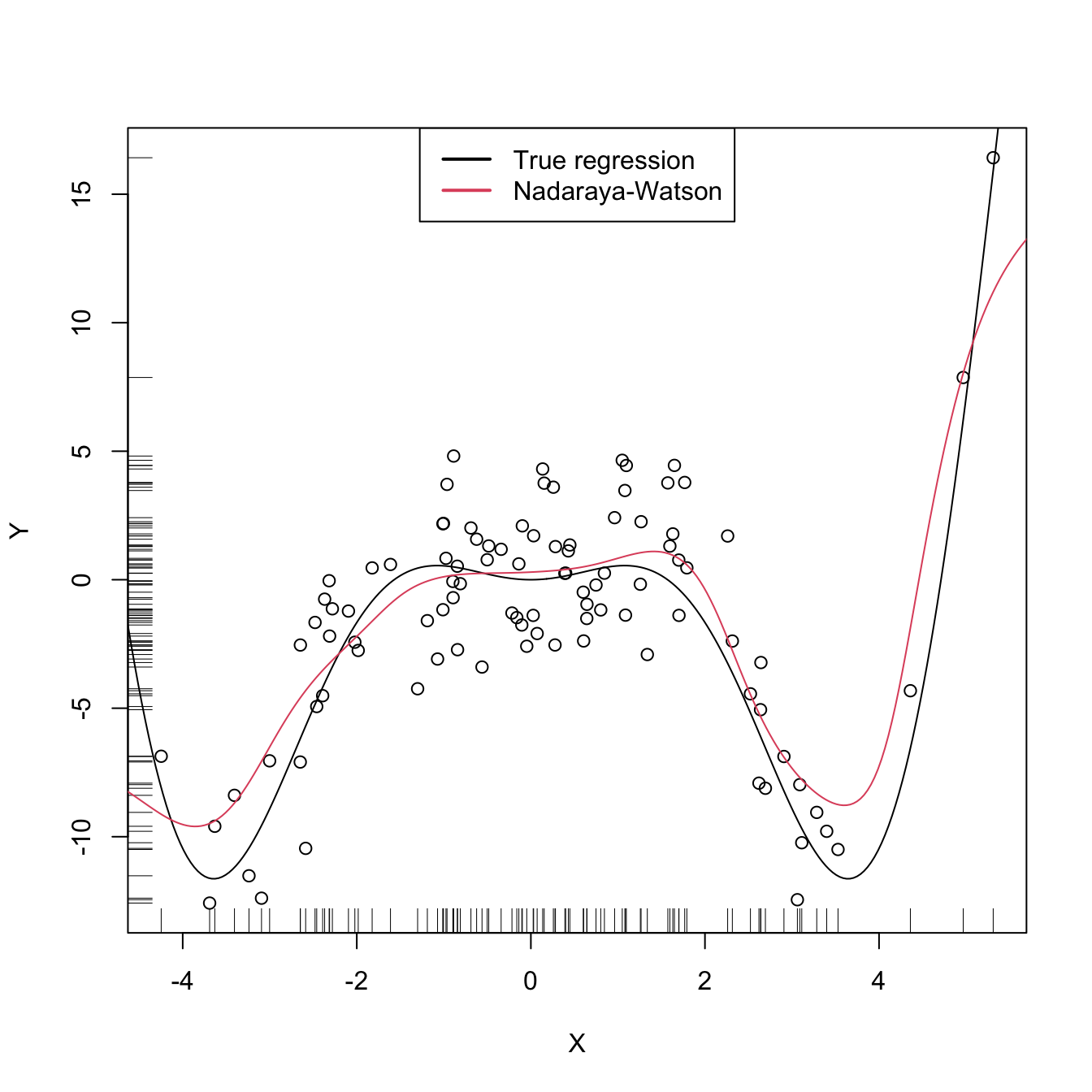

$The Nadaraya–Watson estimator of an arbitrary regression function $m.$ Observe how the Nadaraya–Watson estimator is able to estimate the nonlinear form of the regression function without prior knowledge about its shape.$

Figure 4.1: The Nadaraya–Watson estimator of an arbitrary regression function $m.$ Observe how the Nadaraya–Watson estimator is able to estimate the nonlinear form of the regression function without prior knowledge about its shape.

Exercise 4.3 Implement an R function with your own version of the Nadaraya–Watson estimator and compare it with the nw function. Your objective is to improve the efficiency of nw as much as possible by rethinking its implementation. Focus only in the Nadaraya–Watson estimator with normal kernel, removing the kernel argument from your function. You may reduce the accuracy of the estimator up to 1e-7 to achieve better efficiency. Use the microbenchmark::microbenchmark function to measure the running times for a sample of size $n=10,000.$

Similarly to kernel density estimation, in the Nadaraya–Watson estimator the bandwidth has a prominent effect on the shape of the estimator, whereas the kernel is clearly less important. The code below illustrates the effect of varying $h$ using the manipulate::manipulate function.

# Effect of h on Nadaraya-Watson fits
manipulate::manipulate({

  # Plot data
  plot(X, Y)
  rug(X, side = 1)
  rug(Y, side = 2)
  lines(x_grid, m(x_grid), col = 1)
  lines(x_grid, nw(x = x_grid, X = X, Y = Y, h = h), col = 2)
  legend("topright", legend = c("True regression", "Nadaraya-Watson"),
         lwd = 2, col = 1:2)

}, h = manipulate::slider(min = 0.01, max = 10, initial = 0.5, step = 0.01))

4.1.2 Local polynomial estimator

The Nadaraya–Watson estimator can be seen as a particular case of a wider class of nonparametric estimators, the so-called local polynomial estimators. Specifically, Nadaraya–Watson is the one that corresponds to performing a local constant fit. Let’s see this wider class of nonparametric estimators and their advantages with respect to the Nadaraya–Watson estimator.

A motivation for the local polynomial fit comes from attempting to find an estimator $\hat{m}$ of $m$ that “minimizes”¹²⁶ the Residual Sum of Squares (RSS)

\[\begin{align} \sum_{i=1}^n(Y_i-\hat{m}(X_i))^2\tag{4.6} \end{align}\]

without assuming any particular form for the underlying $m.$ This is not achievable directly, since no knowledge about $m$ is available. Recall that what it was done in parametric models, such as linear regression (see Section B.1), was to assume a parametrization for $m$ (e.g., $m_{\boldsymbol{\beta}}(\mathbf{x})=\beta_0+\beta_1x$ for the simple linear model) which allowed tackling the minimization of (4.6) by means of solving

\[\begin{align*} m_{\hat{\boldsymbol{\beta}}}(\mathbf{x}):=\arg\min_{\boldsymbol{\beta}}\sum_{i=1}^n(Y_i-m_{\boldsymbol{\beta}}(X_i))^2. \end{align*}\]

When $m$ has no parametrization available and can adopt any mathematical form, an alternative approach is required. The first step is to induce a local parametrization on $m.$ By a $p$-th¹²⁷ order Taylor expansion it is possible to obtain that, for $x$ close to $X_i,$

\[\begin{align} m(X_i)\approx&\, m(x)+m'(x)(X_i-x)+\frac{m''(x)}{2}(X_i-x)^2\nonumber\\ &+\cdots+\frac{m^{(p)}(x)}{p!}(X_i-x)^p.\tag{4.7} \end{align}\]

Then, plugging (4.7) in the population version of (4.6) that replaces $\hat{m}$ with $m,$ we have that

\[\begin{align} \sum_{i=1}^n\left(Y_i-\sum_{j=0}^p\frac{m^{(j)}(x)}{j!}(X_i-x)^j\right)^2.\tag{4.8} \end{align}\]

This expression is still not workable: it depends on $m^{(j)}(x),$ $j=0,\ldots,p,$ which of course are unknown, as $m$ is unknown. The key idea now is:

Set $\beta_j:=\frac{m^{(j)}(x)}{j!}$ and turn (4.8) into a linear regression problem where the unknown parameters are precisely $\boldsymbol{\beta}=(\beta_0,\beta_1,\ldots,\beta_p)^\top.$

Simply rewriting (4.8) using this idea gives

\[\begin{align} \sum_{i=1}^n\left(Y_i-\sum_{j=0}^p\beta_j(X_i-x)^j\right)^2.\tag{4.9} \end{align}\]

Now, estimates for $\boldsymbol{\beta}$ automatically produce estimates for $m^{(j)}(x),$ $j=0,\ldots,p.$ In addition, we know how to obtain an estimate $\hat{\boldsymbol{\beta}}$ that minimizes (4.9), since this is precisely the least squares problem studied in linear models.¹²⁸ The final touch is to weight the contributions of each datum $(X_i,Y_i)$ to the estimation of $m(x)$ according to the proximity of $X_i$ to $x.$¹²⁹ We can achieve this precisely with kernels:

\[\begin{align} \hat{\boldsymbol{\beta}}_h:=\arg\min_{\boldsymbol{\beta}\in\mathbb{R}^{p+1}}\sum_{i=1}^n\left(Y_i-\sum_{j=0}^p\beta_j(X_i-x)^j\right)^2K_h(x-X_i).\tag{4.10} \end{align}\]

Solving (4.10) is easy once the proper notation is introduced. To that end, denote

\[\begin{align*} \mathbf{X}:=\begin{pmatrix} 1 & X_1-x & \cdots & (X_1-x)^p\\ \vdots & \vdots & \ddots & \vdots\\ 1 & X_n-x & \cdots & (X_n-x)^p\\ \end{pmatrix}_{n\times(p+1)} \end{align*}\]

and

\[\begin{align*} \mathbf{W}:=\mathrm{diag}(K_h(X_1-x),\ldots, K_h(X_n-x)),\quad \mathbf{Y}:=\begin{pmatrix} Y_1\\ \vdots\\ Y_n \end{pmatrix}_{n\times 1}. \end{align*}\]

Then we can re-express (4.10) into a weighted least squares problem, which has an exact solution:

\[\begin{align} \hat{\boldsymbol{\beta}}_h&=\arg\min_{\boldsymbol{\beta}\in\mathbb{R}^{p+1}} (\mathbf{Y}-\mathbf{X}\boldsymbol{\beta})^\top\mathbf{W}(\mathbf{Y}-\mathbf{X}\boldsymbol{\beta})\tag{4.11}\\ &=(\mathbf{X}^\top\mathbf{W}\mathbf{X})^{-1}\mathbf{X}^\top\mathbf{W}\mathbf{Y}.\tag{4.12} \end{align}\]

The estimate¹³⁰ of $m(x)$ is therefore computed as¹³¹

\[\begin{align} \hat{m}(x;p,h):=&\,\hat{\beta}_{h,0}\nonumber\\ =&\,\mathbf{e}_1'(\mathbf{X}^\top\mathbf{W}\mathbf{X})^{-1}\mathbf{X}^\top\mathbf{W}\mathbf{Y}\nonumber\\ =&\,\sum_{i=1}^nW^p_{i}(x)Y_i,\tag{4.13} \end{align}\]

where

\[\begin{align*} W^p_{i}(x):=\mathbf{e}_1'(\mathbf{X}^\top\mathbf{W}\mathbf{X})^{-1}\mathbf{X}^\top\mathbf{W}\mathbf{e}_i \end{align*}\]

and $\mathbf{e}_i$ is the $i$-th canonical vector.¹³² Just as the Nadaraya–Watson was, the local polynomial estimator is a weighted linear combination of the responses.¹³³

Two cases on (4.13) deserve special attention:

$p=0$ is the local constant estimator, previously referred to as the Nadaraya–Watson estimator. In this situation, the estimator has explicit weights, as we saw before:

\[\begin{align} W_i^0(x)=\frac{K_h(x-X_i)}{\sum_{j=1}^nK_h(x-X_j)}.\tag{4.14} \end{align}\]
$p=1$ is the local linear estimator, which has weights equal to

\[\begin{align} W_i^1(x)=\frac{1}{n}\frac{\hat{s}_2(x;h)-\hat{s}_1(x;h)(X_i-x)}{\hat{s}_2(x;h)\hat{s}_0(x;h)-\hat{s}_1(x;h)^2}K_h(x-X_i),\tag{4.15} \end{align}\]

where $\hat{s}_r(x;h):=\frac{1}{n}\sum_{i=1}^n(X_i-x)^rK_h(x-X_i).$

Exercise 4.4 Show that (4.12) is the solution of (4.11), $\hat{\boldsymbol{\beta}}_h.$ To do so, first prove Exercise B.1.

Exercise 4.5 Show that the local polynomial estimator yields the Nadaraya–Watson estimator when $p=0.$ Use (4.12) to obtain (4.5).

Exercise 4.6 Prove that:

$\sum_{i=1}^nW_i^0(x)=1$ and $W_i^0(x)\geq0$ for all $i=1,\ldots,n$ (weighted mean).
$\sum_{i=1}^nW_i^1(x)=1$ and $W_i^1(x)\not\geq0$ for all $i=1,\ldots,n$ (not a weighted mean). Give an example of positive and negative weights.

Exercise 4.7 Obtain the weight expressions (4.15) of the local linear estimator using the matrix inversion formula for $2\times2$ matrices: $\begin{pmatrix}a & b\\ c & d\end{pmatrix}^{-1}=(ad-bc)^{-1}\begin{pmatrix}d & -b\\ -c & a\end{pmatrix}.$

Remark. The local polynomial fit is computationally more expensive than the local constant fit: $\hat{m}(x;p,h)$ is obtained as the solution of a weighted linear problem, whereas $\hat{m}(x;0,h)$ can directly be computed as a weighted mean of the responses. Even if the explicit form (4.15) is available when $p=1,$ (4.15) is roughly three times more costly than (4.14) (recall the $\hat{s}_r(x;h),$ $r=0,1,2$). The computational demand escalates with $p,$ since computing $\hat{m}(x;p,h)$ requires inverting the $p\times p$ matrix $\mathbf{X}^\top\mathbf{W}\mathbf{X}.$

The local polynomial estimator $\hat{m}(\cdot;p,h)$ of $m$ performs a series of weighted polynomial fits, as many as points $x$ on which $\hat{m}(\cdot;p,h)$ is to be evaluated.

Figure 4.2 illustrates the construction of the local polynomial estimator (up to cubic degree) and shows how $\hat\beta_0=\hat{m}(x;p,h),$ the intercept of the local fit, estimates $m$ at $x$ by constructing a local polynomial fit in the neighborhood of $x.$

Figure 4.2: Construction of the local polynomial estimator. The animation shows how local polynomial fits in a neighborhood of $x$ are combined to provide an estimate of the regression function, which depends on the polynomial degree, bandwidth, and kernel (gray density at the bottom). The data points are shaded according to their weights for the local fit at $x.$ Application available here.

An inefficient implementation of the local polynomial estimator can be done relatively straightforwardly from the previous insights and from expression (4.12). However, several R packages provide implementations, such as KernSmooth::locpoly and R’s loess¹³⁴ (but this one has a different control of the bandwidth plus a set of other modifications). Below are some examples of their use.

# Generate some data
set.seed(123456)
n <- 100
eps <- rnorm(n, sd = 2)
m <- function(x) x^3 * sin(x)
X <- rnorm(n, sd = 1.5)
Y <- m(X) + eps
x_grid <- seq(-10, 10, l = 500)

# KernSmooth::locpoly fits
h <- 0.25
lp0 <- KernSmooth::locpoly(x = X, y = Y, bandwidth = h, degree = 0,
                           range.x = c(-10, 10), gridsize = 500)
lp1 <- KernSmooth::locpoly(x = X, y = Y, bandwidth = h, degree = 1,
                           range.x = c(-10, 10), gridsize = 500)
# Provide the evaluation points through range.x and gridsize

# loess fits
span <- 0.25 # The default span is 0.75, which works very bad in this scenario
lo0 <- loess(Y ~ X, degree = 0, span = span)
lo1 <- loess(Y ~ X, degree = 1, span = span)
# loess employs a "span" argument that plays the role of a variable bandwidth
# "span" gives the proportion of points of the sample that are taken into
# account for performing the local fit about x and then uses a triweight kernel
# (not a normal kernel) for weighting the contributions. Therefore, the final
# estimate differs from the definition of local polynomial estimator, although
# the principles in which are based are the same

# Prediction at x = 2
x <- 2
lp1$y[which.min(abs(lp1$x - x))] # Prediction by KernSmooth::locpoly
## [1] 5.445975
predict(lo1, newdata = data.frame(X = x)) # Prediction by loess
##        1 
## 5.379652
m(x) # True regression
## [1] 7.274379

# Plot data
plot(X, Y)
rug(X, side = 1)
rug(Y, side = 2)
lines(x_grid, m(x_grid), col = 1)
lines(lp0$x, lp0$y, col = 2)
lines(lp1$x, lp1$y, col = 3)
lines(x_grid, predict(lo0, newdata = data.frame(X = x_grid)), col = 2, lty = 2)
lines(x_grid, predict(lo1, newdata = data.frame(X = x_grid)), col = 3, lty = 2)
legend("bottom", legend = c("True regression", "Local constant (locpoly)",
                            "Local linear (locpoly)", "Local constant (loess)",
                            "Local linear (loess)"),
       lwd = 2, col = c(1:3, 2:3), lty = c(rep(1, 3), rep(2, 2)))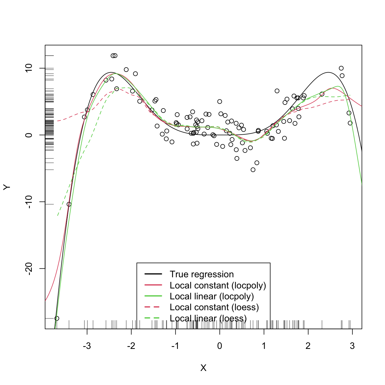

Exercise 4.8 Perform the following tasks:

Implement your own version of the local linear estimator. The function must take a sample X, a sample Y, the points x at which the estimate is to be obtained, the bandwidth h, and the kernel K.
Test its correct behavior by estimating an artificial dataset (e.g., the one considered in Exercise 4.16) that follows a linear model.

As with the Nadaraya–Watson, the local polynomial estimator heavily depends on $h.$ The code below illustrates the effect of varying $h$ using the manipulate::manipulate function.

# Effect of h on local polynomial fits
manipulate::manipulate({

  # Plot data
  lpp <- KernSmooth::locpoly(x = X, y = Y, bandwidth = h, degree = p,
                             range.x = c(-10, 10), gridsize = 500)
  plot(X, Y)
  rug(X, side = 1)
  rug(Y, side = 2)
  lines(x_grid, m(x_grid), col = 1)
  lines(lpp$x, lpp$y, col = p + 2)
  legend("bottom", legend = c("True regression", "Local polynomial fit"),
         lwd = 2, col = c(1, p + 2))

}, p = manipulate::slider(min = 0, max = 4, initial = 0, step = 1),
h = manipulate::slider(min = 0.01, max = 10, initial = 0.5, step = 0.01))

A more sophisticated framework for performing nonparametric estimation of the regression function is the np package, which is introduced in detail in Section 4.5. This package will be the approach chosen for the more challenging situation in which several predictors are present, since the former implementations (KernSmooth::locpoly, loess, and our own implementations) do not scale well for more than one predictor.

Exercise 4.9 Perform the following tasks:

Code your own implementation of the local cubic estimator. The function must take as input the vector of evaluation points x, the sample data, and the bandwidth h. Use the normal kernel. The result must be a vector of the same length as x containing the estimator evaluated at x.
Test the implementation by estimating the regression function in the location model $Y = m(X)+\varepsilon,$ where $m(x)=(x-1)^2,$ $X\sim\mathcal{N}(1,1),$ and $\varepsilon\sim\mathcal{N}(0,0.5).$ Do it for a sample of size $n=500.$

4.2 Asymptotic properties

The asymptotic properties of the local polynomial estimator give us valuable insights into its performance. In particular, they allow answering, precisely, the following questions:

What affects the performance of the local polynomial estimator? Is local linear estimation better than local constant estimation? What is the effect of $h$ on the estimates?

The asymptotic analysis of the local constant and local linear estimators¹³⁵ is achieved, as done in Sections 2.3 and 3.3, by examining the asymptotic bias and variance.

In order to establish a framework for the analysis, we consider the so-called location-scale model for $Y$ and its predictor $X$:

\[\begin{align*} Y=m(X)+\sigma(X)\varepsilon, \end{align*}\]

where

\[\begin{align*} \sigma^2(x):=\mathbb{V}\mathrm{ar}[Y \mid X=x] \end{align*}\]

is the conditional variance of $Y$ given $X,$ and $\varepsilon$ is such that $\mathbb{E}[\varepsilon]=0$ and $\mathbb{V}\mathrm{ar}[\varepsilon]=1.$ Recall that, since the conditional variance is not forced to be constant, we are implicitly allowing for heteroscedasticity.¹³⁶

Note that for the derivation of the Nadaraya–Watson estimator and the local polynomial estimator we did not assume any particular assumption, beyond the (implicit) differentiability of $m$ up to order $p$ for the local polynomial estimator. The following assumptions¹³⁷ are the only requirements to perform the asymptotic analysis of the estimator:

A1.¹³⁸ $m$ is twice continuously differentiable.
A2.¹³⁹ $\sigma^2$ is continuous and positive.
A3.¹⁴⁰ $f,$ the marginal pdf of $X,$ is continuously differentiable and bounded away from zero.¹⁴¹
A4.¹⁴² The kernel $K$ is a symmetric and bounded pdf with finite second moment and is square integrable.
A5.¹⁴³ $h=h_n$ is a deterministic sequence of bandwidths such that, when $n\to\infty,$ $h\to0$ and $nh\to\infty.$

The bias and variance are studied in their conditional versions on the predictor’s sample $X_1,\ldots,X_n.$ The reason for analyzing the conditional instead of the unconditional versions is to avoid technical difficulties that integration with respect to the unknown predictor’s density may pose. This is in the spirit of what was done in parametric inference (observe Sections B.1.2 and B.2.2).

The main result follows. It provides useful insights into the effect of $p,$ $m,$ $f$ (standing from now on for the marginal pdf of $X$), and $\sigma^2$ in the performance of $\hat{m}(\cdot;p,h)$ for $p=0,1.$

Theorem 4.1 Under A1–A5, the conditional bias and variance of the local constant ($p=0$) and local linear ($p=1$) estimators are

\[\begin{align} \mathrm{Bias}[\hat{m}(x;p,h) \mid X_1,\ldots,X_n]&=B_p(x)h^2+o_\mathbb{P}(h^2),\tag{4.16}\\ \mathbb{V}\mathrm{ar}[\hat{m}(x;p,h) \mid X_1,\ldots,X_n]&=\frac{R(K)}{nhf(x)}\sigma^2(x)+o_\mathbb{P}((nh)^{-1}),\tag{4.17} \end{align}\]

where

\[\begin{align*} B_p(x):=\begin{cases} \frac{\mu_2(K)}{2}\left\{m''(x)+2\frac{m'(x)f'(x)}{f(x)}\right\},&\text{ if }p=0,\\ \frac{\mu_2(K)}{2}m''(x),&\text{ if }p=1. \end{cases} \end{align*}\]

Remark. The little-$o_\mathbb{P}$s in (4.16) and (4.17) appear (instead of little-$o$s as in Theorem 2.1) because $\mathrm{Bias}[\hat{m}(x;p,h) \mid X_1,\ldots,X_n]$ and $\mathbb{V}\mathrm{ar}[\hat{m}(x;p,h) \mid X_1,\ldots,X_n]$ are random variables. Then, the asymptotic expansions of these random variables have stochastic remainders that converge to zero in probability at specific rates.

The bias and variance expressions (4.16) and (4.17) yield very interesting insights:

Bias:
- The bias decreases with $h$ quadratically for both $p=0,1.$ That means that small bandwidths $h$ give estimators with low bias, whereas large bandwidths provide largely biased estimators.
- For $p=1,$ the bias at $x$ is directly proportional to $m''(x).$ Therefore:
  - The bias is negative in regions where $m$ is concave, i.e., $\{x\in\mathbb{R}:m''(x)<0\}.$ These regions correspond to peaks and local maxima of $m.$
  - Conversely, the bias is positive in regions where $m$ is convex, i.e., $\{x\in\mathbb{R}:m''(x)>0\}.$ These regions correspond to valleys and local minima of $m.$
  - All in all, the “wilder” the curvature of $m,$ the larger the bias and the harder to estimate $m$.
- For $p=0,$ the bias at $x$ is more convoluted and is affected by $m''(x),$ $m'(x),$ $f'(x),$ and $f(x)$:
  - The quantities $m'(x),$ $f'(x),$ and $f(x)$ are not present in the bias when $p=1.$ Precisely, for the local constant estimator, the lower the density $f(x),$ the larger the bias (in absolute value). Also, the faster $m$ and $f$ change at $x$ (derivatives), the larger the bias. Thus the bias of the local constant estimator is sensitive to $m'(x)$ and $f(x)$, unlike the local linear estimator (which is sensitive to $m''(x)$ only). Particularly, the fact that the bias of the local constant estimator depends on $f'(x)$ and $f(x)$ is referred to as the design bias since it depends merely on the predictor’s distribution.
  - The quantity $m''(x)$ contributes to the bias in the same way as it does for $p = 1,$ this contribution being negative in regions corresponding to peaks and local maxima of $m,$ and positive in the valleys and local minima of $m.$ In general, the “wilder” the curvature of $m,$ the larger its contribution to the bias and the harder to estimate $m.$
Variance:
- The main term of the variance is the same for $p=0,1$. In addition, it depends directly on $\frac{\sigma^2(x)}{f(x)}.$ As a consequence, the lower the density, the more variable $\hat{m}(x;p,h)$ is.¹⁴⁴ Also, the larger the conditional variance at $x,$ $\sigma^2(x),$ the more variable $\hat{m}(x;p,h)$ is.¹⁴⁵
- The variance decreases as a factor of $(nh)^{-1}$. This is related to the so-called effective sample size $nh,$ which can be thought of as the amount of data in the neighborhood of $x$ that is employed for performing the regression.¹⁴⁶

All in all, the main takeaway of the analysis of $p=0$ vs. $p=1$ is:

$p=1$ has, in general, smaller bias than that of $p=0$ (but of the same order) while keeping the same variance as $p=0$.

An extended version of Theorem 4.1, given in Theorem 3.1 in Fan and Gijbels (1996), shows that this phenomenon extends to higher orders: odd order ($p=2\nu+1,$ $\nu\in\mathbb{N}$) polynomial fits introduce an extra coefficient for the polynomial fit that allows them to reduce the bias, while maintaining the same variance of the preceding¹⁴⁷ even order ($p=2\nu$). So, for example, local cubic fits are preferred to local quadratic fits. This motivates the following motto: local polynomial fitting is an odd world (Fan and Gijbels (1996)).

Finally, we have the asymptotic pointwise normality of the estimator, an analogous result to Theorem 2.2 which is helpful to obtain pointwise confidence intervals for $m$ afterwards.

Theorem 4.2 Assume that $\mathbb{E}[(Y-m(x))^{2+\delta} \mid X=x]<\infty$ for some $\delta>0.$ Then, under A1–A5,

\[\begin{align} &\sqrt{nh}(\hat m(x;p,h)-\mathbb{E}[\hat m(x;p,h) \mid X_1,\ldots,X_n])\stackrel{d}{\longrightarrow}\mathcal{N}\left(0,\frac{R(K)\sigma^2(x)}{f(x)}\right).\tag{4.18}\end{align}\]

Additionally, if $nh^5=O(1),$ then

\[\begin{align} &\sqrt{nh}\left(\hat m(x;p,h)-m(x)-B_p(x)h^2\right)\stackrel{d}{\longrightarrow}\mathcal{N}\left(0,\frac{R(K)\sigma^2(x)}{f(x)}\right).\tag{4.19} \end{align}\]

Exercise 4.10 Theorem 4.1 gives some additional insights with respect to $B_p(x),$ the dominating term of the bias:

If $m$ is constant,¹⁴⁸ then $B_0(x)=0.$
If $m$ is linear,¹⁴⁹ then $B_1(x)=0.$

That is, for each of these two cases, $\mathrm{Bias}[\hat{m}(x;p,h) \mid X_1,\ldots,X_n]=o_\mathbb{P}(h^2).$ The local constant and local linear estimators are actually exactly unbiased when estimating constant and linear regression functions, respectively. That is, $\mathbb{E}_c[\hat{m}(x;0,h) \mid X_1,\ldots,X_n]=c$ and $\mathbb{E}_{a,b}[\hat{m}(x;1,h) \mid X_1,\ldots,X_n]=ax+b,$ where $\mathbb{E}_c[\cdot \mid X_1,\ldots,X_n]$ and $\mathbb{E}_{a,b}[\cdot \mid X_1,\ldots,X_n]$ represent the conditional expectations under the constant and linear models, respectively. Prove these two results.

4.3 Bandwidth selection

Bandwidth selection, as for kernel density estimation, is of key practical importance for kernel regression estimation. Several bandwidth selectors have been proposed for kernel regression by following plug-in and cross-validatory ideas that are similar to the ones seen in Section 2.4. For the sake of simplicity, we first briefly overview the plug-in analogues for local linear regression for a single continuous predictor. Then, the main focus will be placed on Least Squares Cross-Validation (LSCV; simply referred to as CV), as the cross-validation methodology readily generalizes to the more complex settings to be seen in Section 5.1.

As in the kde case, the first step for performing bandwidth selection is to define an error criterion suitable for the estimator $\hat{m}(\cdot;p,h).$ The density-weighted ISE of $\hat{m}(\cdot;p,h),$

\[\begin{align*} \mathrm{ISE}[\hat{m}(\cdot;p,h)]:=&\,\int(\hat{m}(x;p,h)-m(x))^2f(x)\,\mathrm{d}x, \end{align*}\]

is often considered. Observe that this definition is very similar to the kde’s ISE, except for the fact that $f$ appears as a weight for the quadratic difference: what matters is to minimize the estimation error on the regions where the density of $X$ is higher. As a consequence, this definition does not give any importance to the errors made by $\hat{m}(\cdot;p,h)$ when estimating $m$ at regions with virtually no data.¹⁵⁰

The ISE of $\hat{m}(\cdot;p,h)$ is a random quantity that directly depends on the sample $(X_1,Y_1),\ldots,(X_n,Y_n).$ In order to avoid this nuisance, the conditional¹⁵¹ MISE of $\hat{m}(\cdot;p,h)$ is often employed:

\[\begin{align*} \mathrm{MISE}[\hat{m}(\cdot;p,h) &\mid X_1,\ldots,X_n]\\ :=&\,\mathbb{E}\left[\mathrm{ISE}[\hat{m}(\cdot;p,h)] \mid X_1,\ldots,X_n\right]\\ =&\,\int\mathbb{E}\left[(\hat{m}(x;p,h)-m(x))^2 \mid X_1,\ldots,X_n\right]f(x)\,\mathrm{d}x\\ =&\,\int\mathrm{MSE}\left[\hat{m}(x;p,h) \mid X_1,\ldots,X_n\right]f(x)\,\mathrm{d}x. \end{align*}\]

Clearly, the goal is to find the bandwidth that minimizes this error,

\[\begin{align*} h_\mathrm{MISE}:=\arg\min_{h>0}\mathrm{MISE}[\hat{m}(\cdot;p,h) \mid X_1,\ldots,X_n], \end{align*}\]

but this is an intractable problem because of the lack of explicit expressions. However, since the MISE follows by integrating the conditional MSE, explicit asymptotic expressions can be found.

In the case of local linear regression, the conditional MSE follows by the conditional squared bias (4.16) and the variance (4.17) given in Theorem 4.1. This produces the conditional AMISE for $\hat{m}(\cdot;p,h),$ $p=0,1$:

\[\begin{align} \mathrm{AMISE}[\hat{m}(\cdot;p,h) \mid X_1,\ldots,X_n]=&\,h^4\int B_p(x)^2f(x)\,\mathrm{d}x\nonumber\\ &+\frac{R(K)}{nh}\int\sigma^2(x)\,\mathrm{d}x.\tag{4.20} \end{align}\]

If $p=1,$ the resulting optimal AMISE bandwidth is

\[\begin{align} h_\mathrm{AMISE}=\left[\frac{R(K)\int\sigma^2(x)\,\mathrm{d}x}{\mu_2^2(K)\theta_{22}(m)n}\right]^{1/5},\tag{4.21} \end{align}\]

where

\[\begin{align*} \theta_{22}(m):=\int(m''(x))^2f(x)\,\mathrm{d}x \end{align*}\]

acts as the “density-weighted curvature of $m$” and completely resembles the curvature term $R(f'')$ that appeared in Section 2.4.

Exercise 4.11 Obtain $\mathrm{AMISE}[\hat{m}(\cdot;p,h) \mid X_1,\ldots,X_n]$ in (4.20) from Theorem 4.1.

Exercise 4.12 Obtain the expression for $h_\mathrm{AMISE}$ in (4.21) from $\mathrm{AMISE}[\hat{m}(\cdot;1,h) \mid X_1,\ldots,X_n].$ Then, obtain the corresponding AMISE optimal bandwidth for $\hat{m}(\cdot;0,h).$

As happened in the density setting, the AMISE-optimal bandwidth cannot be readily employed, as knowledge about the curvature of $m,$ $\theta_{22}(m),$ is required. To make things worse, (4.21) also depends on the integrated conditional variance $\int\sigma^2(x)\,\mathrm{d}x,$ which is unknown too.

4.3.1 Plug-in rules

A possibility to estimate $\theta_{22}(m)$ and $\int\sigma^2(x)\,\mathrm{d}x,$ in the spirit of the normal scale bandwidth selector (or zero-stage plug-in selector) seen in Section 2.4.1, is presented in Section 4.2 in Fan and Gijbels (1996). There, a global parametric fit based on a fourth-order¹⁵² polynomial is employed:

\[\begin{align*} \hat{m}_Q(x)=\hat{\alpha}_0+\sum_{j=1}^4\hat{\alpha}_jx^j, \end{align*}\]

where $\hat{\boldsymbol{\alpha}}$ is obtained from $(X_1,Y_1),\ldots,(X_n,Y_n).$ The second derivative of this quartic fit is

\[\begin{align*} \hat{m}_Q''(x)=2\hat{\alpha}_2+6\hat{\alpha}_3x+12\hat{\alpha}_4x^2. \end{align*}\]

Besides, $\theta_{22}(m)$ can be written in terms of an expectation, which motivates its estimation by Monte Carlo:

\[\begin{align*} \theta_{22}(m)=\mathbb{E}[(m''(X))^2]\approx\frac{1}{n}\sum_{i=1}^n(m''(X_i))^2=:\hat{\theta}_{22}(m). \end{align*}\]

Therefore, combining both estimations we can substitute $\theta_{22}(m)$ with $\hat{\theta}_{22}(\hat{m}_Q)$ in (4.21).

It remains to estimate $\int\sigma^2(x)\,\mathrm{d}x,$ which we can do by assuming homoscedasticity and then estimating the common variance by¹⁵³

\[\begin{align*} \hat{\sigma}_Q^2:=\frac{1}{n-5}\sum_{i=1}^n(Y_i-\hat{m}_Q(X_i))^2. \end{align*}\]

In addition, if we assume that the variance is zero outside the support of $X$ (where there is no data), we can replace $\int\sigma^2(x)\,\mathrm{d}x$ with the estimate $(X_{(n)}-X_{(1)})\hat{\sigma}_Q^2\,$¹⁵⁴ and obtain the Rule-of-Thumb bandwidth selector (RT)

\[\begin{align*} \hat{h}_\mathrm{RT}=\left[\frac{R(K)(X_{(n)}-X_{(1)})\hat{\sigma}_Q^2}{\mu_2^2(K)\hat{\theta}_{22}(\hat{m}_Q)n}\right]^{1/5}. \end{align*}\]

The following code illustrates how to implement this simple selector.

# Evaluation grid
x_grid <- seq(0, 5, l = 500)

# Quartic-like regression function
m <- function(x) 5 * dnorm(x, mean = 1.5, sd = 0.25) - x

# # Highly nonlinear regression function
# m <- function(x) x * sin(2 * pi * x)

# # Quartic regression function (but expressed in an orthogonal polynomial)
# coefs <- attr(poly(x_grid / 5 * 3, degree = 4), "coefs")
# m <- function(x) 20 * poly(x, degree = 4, coefs = coefs)[, 4]

# # Seventh orthogonal polynomial
# coefs <- attr(poly(x_grid / 5 * 3, degree = 7), "coefs")
# m <- function(x) 20 * poly(x, degree = 7, coefs = coefs)[, 7]

# Generate some data
set.seed(123456)
n <- 250
eps <- rnorm(n)
X <- abs(rnorm(n))
Y <- m(X) + eps

# Rule-of-thumb selector
h_RT <- function(X, Y) {

  # Quartic fit
  mod_Q <- lm(Y ~ poly(X, raw = TRUE, degree = 4))

  # Estimates of unknown quantities
  int_sigma2_hat <- diff(range(X)) * sum(mod_Q$residuals^2) / mod_Q$df.residual
  theta_22_hat <- mean((2 * mod_Q$coefficients[3] +
                        6 * mod_Q$coefficients[4] * X +
                        12 * mod_Q$coefficients[5] * X^2)^2)

  # h_RT
  R_K <- 0.5 / sqrt(pi)
  ((R_K * int_sigma2_hat) / (theta_22_hat * length(X)))^(1 / 5)

}

# Selected bandwidth
(h_ROT <- h_RT(X = X, Y = Y))
## [1] 0.1111711

# Local linear fit
lp1_RT <- KernSmooth::locpoly(x = X, y = Y, bandwidth = h_ROT, degree = 1,
                              range.x = c(0, 10), gridsize = 500)

# Quartic fit employed
mod_Q <- lm(Y ~ poly(X, raw = TRUE, degree = 4))

# Plot data
plot(X, Y, ylim = c(-6, 8))
rug(X, side = 1)
rug(Y, side = 2)
lines(x_grid, m(x_grid), col = 1)
lines(lp1_RT$x, lp1_RT$y, col = 2)
lines(x_grid, mod_Q$coefficients[1] +
        poly(x_grid, raw = TRUE, degree = 4) %*% mod_Q$coefficients[-1],
      col = 3)
legend("topright", legend = c("True regression", "Local linear (RT)",
                              "Quartic fit"),
       lwd = 2, col = 1:3)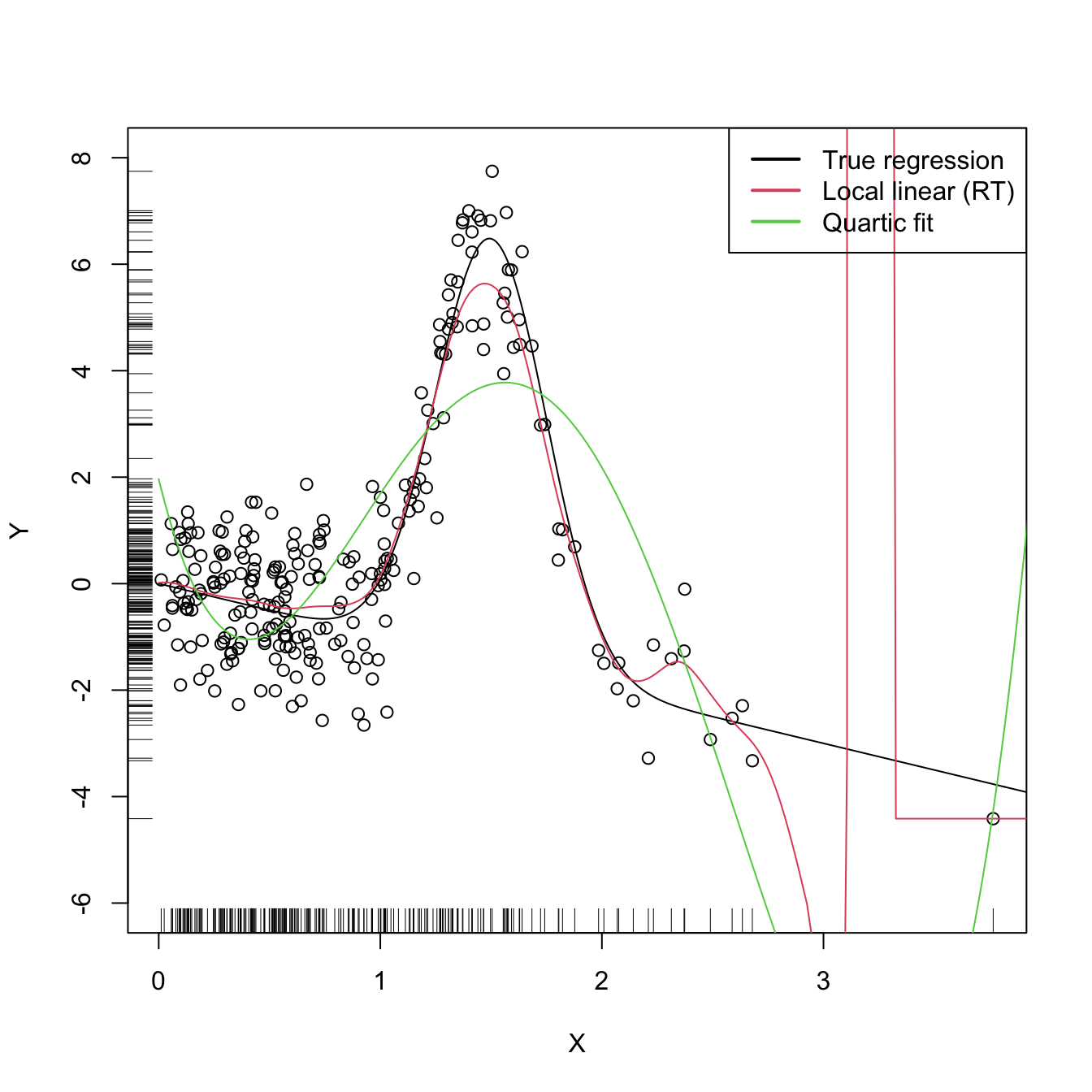

$Local linear estimator with $\hat{h}_\mathrm{RT}$ bandwidth and the quartic global fit. Observe how the local linear estimator behaves erratically at regions with no data – a fact due to the strong dependence of the locally weighted linear regression on few observations.$

Figure 4.3: Local linear estimator with $\hat{h}_\mathrm{RT}$ bandwidth and the quartic global fit. Observe how the local linear estimator behaves erratically at regions with no data – a fact due to the strong dependence of the locally weighted linear regression on few observations.

The $\hat{h}_\mathrm{RT}$ selector strongly depends on how well the curvature of $m$ is approximated by the quartic fit. In addition, it assumes that the conditional variance is constant, which may be unrealistic. The exercise below intends to illustrate these limitations.

Exercise 4.13 Explore in the code above the effect of the regression function, and visualize how poor quartic fits tend to give poor nonparametric fits. Then, adapt the sampling mechanism to introduce heteroscedasticity on $Y$ and investigate the behavior of the nonparametric estimator based on $\hat{h}_\mathrm{RT}.$

The rule-of-thumb selector is a zero-stage plug-in selector. An $\ell$-stage plug-in selector was proposed by Ruppert, Sheather, and Wand (1995)¹⁵⁵ and shares the same spirit of the DPI bandwidth selector seen in Section 2.4.1. As a consequence, the DPI selector for kre turns (4.21) into a usable selector by following a known agenda: it employs a series of optimal nonparametric estimations of $\theta_{22}(m)$ that depend on high-order curvature terms $\theta_{rs}(m):=\int m^{(r)}(x)m^{(s)}(x)f(x)\,\mathrm{d}x,$ ending this iterative procedure with a parametric estimation of a higher-order curvature.

The kind of parametric fit employed is a “block quartic fit”. This is a series of $N$ different quartic fits $\hat{m}_{Q,1},\ldots,\hat{m}_{Q,N}$ of the regression function $m$ that are done in $N$ blocks of the data. These blocks are defined by sorting the sample $X_1,\ldots,X_n$ and then partitioning it into approximately $N$ blocks of equal size $n/N.$ The purpose of the block quartic fit is to achieve more flexibility in the estimation of the curvature¹⁵⁶ terms $\theta_{22}(m)$ and $\theta_{24}(m).$ The estimation of $\int\sigma^2(x)\,\mathrm{d}x$ is carried out by pooling the individual estimates of the conditional variance in the $N$ blocks, $\hat{\sigma}^2_{Q,1},\ldots,\hat{\sigma}^2_{Q,N},$ and by assuming a compactly supported density $f.$¹⁵⁷ The selection of $N$ can be done in a data-driven way by relying on a model selection criterion (see Ruppert, Sheather, and Wand (1995)), such as the AIC or BIC.

The resulting bandwidth selector, $\hat{h}_\mathrm{DPI},$ has a much faster convergence rate to $h_{\mathrm{MISE}}$ than cross-validatory selectors. However, it is notably more convoluted, and as a consequence it is less straightforward to extend to more complex settings.¹⁵⁸

The DPI selector for the local linear estimator is implemented in KernSmooth::dpill.

# Generate some data
set.seed(123456)
n <- 250
eps <- rnorm(n)
X <- abs(rnorm(n))
m <- function(x) x * sin(2 * pi * x)
Y <- m(X) + eps

# Selected bandwidth
(h_ROT <- h_RT(X = X, Y = Y))
## [1] 0.3489934

# DPI selector
(h_DPI <- KernSmooth::dpill(x = X, y = Y))
## [1] 0.05172781

# Fits
lp1_RT <- KernSmooth::locpoly(x = X, y = Y, bandwidth = h_ROT, degree = 1,
                              range.x = c(0, 10), gridsize = 500)
lp1_DPI <- KernSmooth::locpoly(x = X, y = Y, bandwidth = h_DPI, degree = 1,
                               range.x = c(0, 10), gridsize = 500)

# Plot data
plot(X, Y, ylim = c(-6, 8))
rug(X, side = 1)
rug(Y, side = 2)
lines(x_grid, m(x_grid), col = 1)
lines(lp1_DPI$x, lp1_DPI$y, col = 2)
lines(lp1_RT$x, lp1_RT$y, col = 3)
legend("topleft", legend = c("True regression", "Local linear (DPI)",
                             "Local linear (RT)"), lwd = 2, col = 1:3)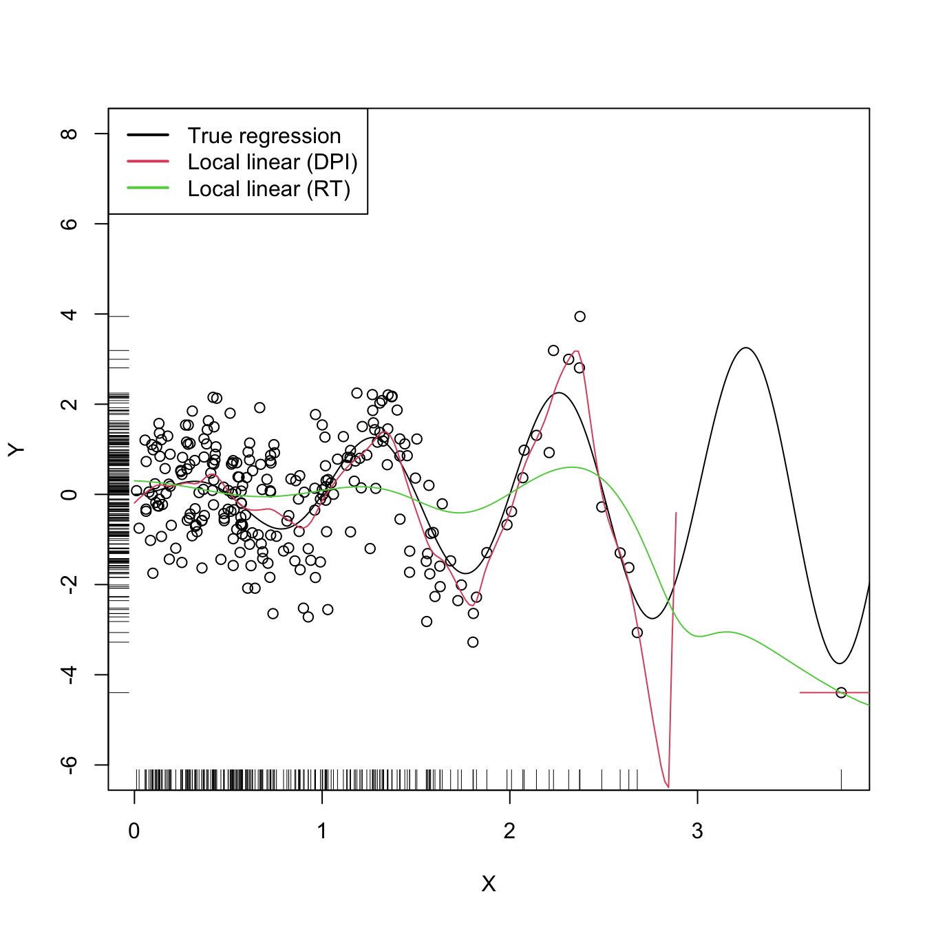

4.3.2 Cross-validation

Following an analogy with the fit of the linear model (see Section B.1.1), an obvious possibility is to select an adequate bandwidth $h$ for $\hat{m}(\cdot;p,h)$ that minimizes a RSS of the form

\[\begin{align} \frac{1}{n}\sum_{i=1}^n(Y_i-\hat{m}(X_i;p,h))^2.\tag{4.22} \end{align}\]

However, this is a bad idea. Contrarily to what happened in the linear model, where it was almost¹⁵⁹ impossible to perfectly fit the data due to the limited flexibility of the model, the infinite flexibility of the local polynomial estimator allows interpolating the data if $h\to0.$ As a consequence, attempting to minimize (4.22) always leads to $h\approx 0,$ which results in a useless interpolation that misses the target of the estimation, $m.$

# Grid for representing (4.22)
h_grid <- seq(0.1, 1, l = 200)^2
error <- sapply(h_grid, function(h) {
  mean((Y - nw(x = X, X = X, Y = Y, h = h))^2)
})

# Error curve
plot(h_grid, error, type = "l")
rug(h_grid)
abline(v = h_grid[which.min(error)], col = 2)

The root of the problem is the comparison of $Y_i$ with $\hat{m}(X_i;p,h),$ since there is nothing that forbids that, when $h\to0,$ $\hat{m}(X_i;p,h)\to Y_i.$ We can change this behavior if we compare $Y_i$ with $\hat{m}_{-i}(X_i;p,h),$¹⁶⁰ the leave-one-out estimate of $m$ computed without the $i$-th datum $(X_i,Y_i),$ yielding the least squares cross-validation error

\[\begin{align} \mathrm{CV}(h):=\frac{1}{n}\sum_{i=1}^n(Y_i-\hat{m}_{-i}(X_i;p,h))^2\tag{4.23} \end{align}\]

and then choose

\[\begin{align*} \hat{h}_\mathrm{CV}:=\arg\min_{h>0}\mathrm{CV}(h). \end{align*}\]

The optimization of (4.23) might seem to be very expensive computationally, since computing $n$ regressions for just a single evaluation of the cross-validation function is required. There is, however, a simple and neat theoretical result that vastly reduces the computational complexity, at the price of increasing the memory demand. This trick allows computing, with a single fit, the cross-validation function evaluated at $h.$

Proposition 4.1 For any $p\geq0,$ the weights of the leave-one-out estimator $\hat{m}_{-i}(x;p,h)=\sum_{\substack{j=1\\j\neq i}}^nW_{-i,j}^p(x)Y_j$ can be obtained from $\hat{m}(x;p,h)=\sum_{i=1}^nW_{i}^p(x)Y_i$:

\[\begin{align} W_{-i,j}^p(x)=\frac{W^p_j(x)}{\sum_{\substack{k=1\\k\neq i}}^nW_k^p(x)}=\frac{W^p_j(x)}{1-W_i^p(x)}.\tag{4.24} \end{align}\]

This implies that

\[\begin{align} \mathrm{CV}(h)=\frac{1}{n}\sum_{i=1}^n\left(\frac{Y_i-\hat{m}(X_i;p,h)}{1-W_i^p(X_i)}\right)^2.\tag{4.25} \end{align}\]

The result can be proved by recalling that $\hat{m}(x;p,h)$ is a linear combination¹⁶¹ of the responses $\{Y_i\}_{i=1}^n.$

Exercise 4.14 Consider the Nadaraya–Watson estimator ($p=0$). Then, show (4.24) using (4.14). From there, conclude the proof of Proposition 4.1.

Exercise 4.15 Prove the second equality in (4.24) for the local linear estimator ($p=1$). From there, prove (4.25). Use (4.15).

Remark. Observe that computing (4.25) requires evaluating the local polynomial estimator at the sample $\{X_i\}_{i=1}^n$ and obtaining $\{W_i^p(X_i)\}_{i=1}^n$ (which are needed to evaluate $\hat{m}(X_i;p,h)$). Both tasks can be achieved simultaneously from the $n\times n$ matrix $\big(W_{i}^p(X_j)\big)_{ij}$ and, if $p=0,$ directly from the symmetric $n\times n$ matrix $\left(K_h(X_i-X_j)\right)_{ij},$ for which the storage cost is $O((n^2-n)/2)$ (the diagonal is constant).

Let’s implement $\hat{h}_\mathrm{CV}$ employing (4.25) for the Nadaraya–Watson estimator.

# Generate some data to test the implementation
set.seed(12345)
n <- 200
eps <- rnorm(n, sd = 2)
m <- function(x) x^2 + sin(x)
X <- rnorm(n, sd = 1.5)
Y <- m(X) + eps
x_grid <- seq(-10, 10, l = 500)

# Objective function
cv_nw <- function(X, Y, h, K = dnorm) {

  sum(((Y - nw(x = X, X = X, Y = Y, h = h, K = K)) /
         (1 - K(0) / colSums(K(outer(X, X, "-") / h))))^2)

}

# Find optimum CV bandwidth, with sensible grid
bw_cv_grid <- function(X, Y,
                       h_grid = diff(range(X)) * (seq(0.05, 0.5, l = 200))^2,
                       K = dnorm, plot_cv = FALSE) {

  # Minimize the CV function on a grid
  obj <- sapply(h_grid, function(h) cv_nw(X = X, Y = Y, h = h, K = K))
  h <- h_grid[which.min(obj)]

  # Add plot of the CV loss
  if (plot_cv) {

    plot(h_grid, obj, type = "o")
    rug(h_grid)
    abline(v = h, col = 2, lwd = 2)

  }

  # CV bandwidth
  return(h)

}

# Bandwidth
h <- bw_cv_grid(X = X, Y = Y, plot_cv = TRUE)

h
## [1] 0.3173499

# Plot result
plot(X, Y)
rug(X, side = 1)
rug(Y, side = 2)
lines(x_grid, m(x_grid), col = 1)
lines(x_grid, nw(x = x_grid, X = X, Y = Y, h = h), col = 2)
legend("top", legend = c("True regression", "Nadaraya-Watson"),
       lwd = 2, col = 1:2)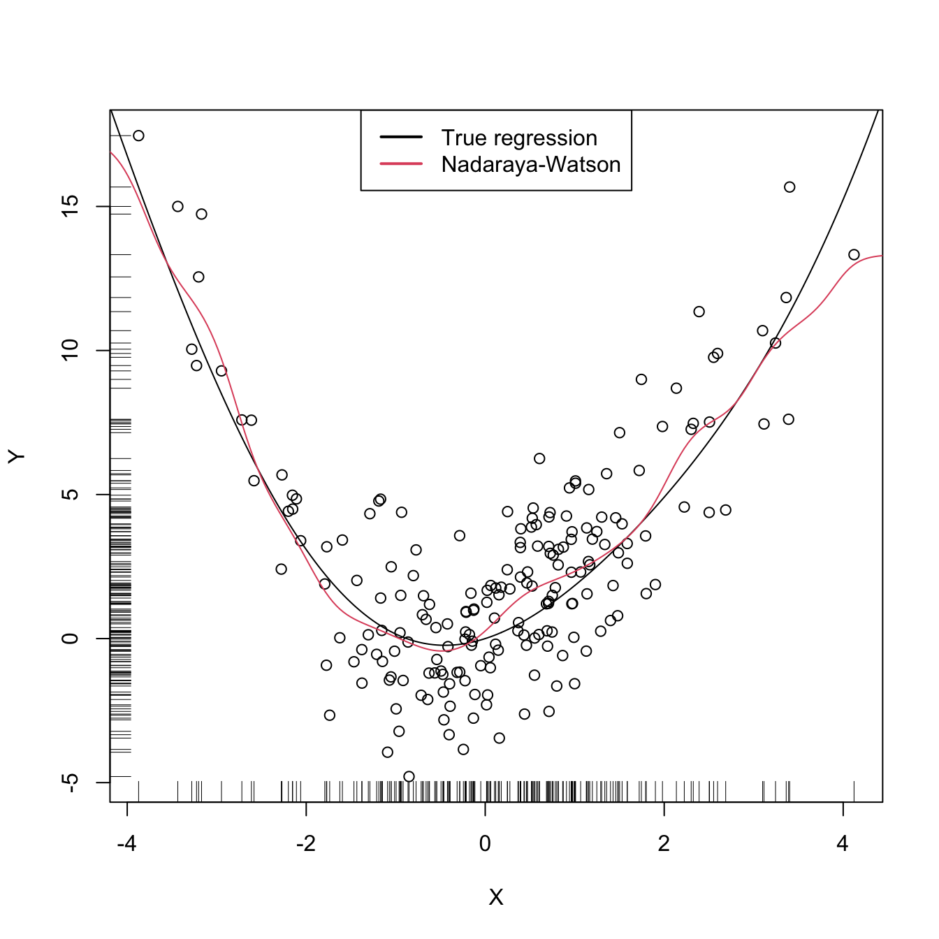

An important warning when computing cross-validation bandwidths is that the objective function can be challenging to minimize and may present several local minima. Therefore, if possible, it is always advisable to graphically inspect the CV loss curve and to run an exhaustive search. When employing an automatic optimization procedure, it is recommended to use several starting values.

The following chunk of code presents the inefficient implementation of $\hat{h}_\mathrm{CV}$ (based on the definition) and evidences its poorer performance.

# Slow objective function
cv_nw_slow <- function(X, Y, h, K = dnorm) {

  sum((Y - sapply(1:length(X), function(i) {
    nw(x = X[i], X = X[-i], Y = Y[-i], h = h, K = K)
    }))^2)

}

# Optimum CV bandwidth, with sensible grid
bw_cv_grid_slow <- function(X, Y, h_grid =
                              diff(range(X)) * (seq(0.05, 0.5, l = 200))^2,
                            K = dnorm, plot_cv = FALSE) {

  # Minimize the CV function on a grid
  obj <- sapply(h_grid, function(h) cv_nw_slow(X = X, Y = Y, h = h, K = K))
  h <- h_grid[which.min(obj)]

  # Add plot of the CV loss
  if (plot_cv) {

    plot(h_grid, obj, type = "o")
    rug(h_grid)
    abline(v = h, col = 2, lwd = 2)

  }

  # CV bandwidth
  return(h)

}

# Same bandwidth
h <- bw_cv_grid_slow(X = X, Y = Y, plot_cv = TRUE)

h
## [1] 0.3173499

# # Time comparison, a factor 10 difference
# microbenchmark::microbenchmark(bw_cv_grid(X = X, Y = Y),
#                                bw_cv_grid_slow(X = X, Y = Y),
#                                times = 10)

Finally, the following chunk of code illustrates the estimation of the regression function of the weight on the mpg in data(Auto, package = "ISLR"), using a cross-validation bandwidth.

# Data -- nonlinear trend
data(Auto, package = "ISLR")
X <- Auto$weight
Y <- Auto$mpg
plot(X, Y, xlab = "weight", ylab = "mpg")


# CV bandwidth
h <- bw_cv_grid(X = X, Y = Y, plot_cv = TRUE)

h
## [1] 110.0398

# Add regression
x_grid <- seq(1600, 5200, by = 10)
plot(X, Y, xlab = "weight", ylab = "mpg")
rug(X, side = 1)
rug(Y, side = 2)
lines(x_grid, nw(x = x_grid, X = X, Y = Y, h = h), col = 2)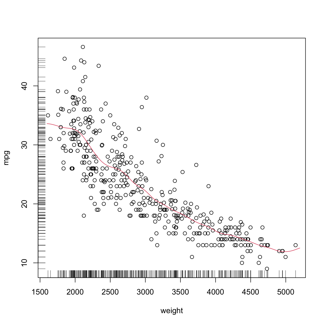

4.4 Regressogram

The regressogram is the adaptation of the histogram to the regression setting. Historically, it has received attention in several applied areas.¹⁶² This and its connection with the histogram are the reasons for its inclusion in this book, since its performance to estimate $m$ is definitely inferior to that of $\hat{m}(\cdot;p,h)$ (see Figure 4.4). The construction described below can be regarded as the opposite path to the one followed in Sections 2.1–2.2 for constructing the kde from the histogram: now we deconstruct the Nadaraya–Watson estimator to obtain the regressogram.

Based on (4.2), the Nadaraya–Watson estimator was constructed by plugging kdes for the joint density of $(X,Y)$ and the marginal density of $X.$ This resulted in

\[\begin{align} \hat{m}(x;0,h)=\frac{\sum_{i=1}^nK_h(x-X_i)Y_i}{\sum_{i=1}^nK_h(x-X_i)}=\frac{\frac{1}{n}\sum_{i=1}^nK_h(x-X_i)Y_i}{\hat{f}(x;h)},\tag{4.26} \end{align}\]

which clearly emphasizes the connection between the kde $\hat{f}(x;h)=\frac{1}{n}\sum_{i=1}^nK_h(x-X_i)$ and $\hat{m}(x;0,h).$ Evidently, this approach gives a smooth estimator for the regression function if the kernels employed in the kde are smooth.

Within (4.26), a possibility is to consider the uniform kernel $K(z)=\frac{1}{2}1_{\{-1<x<1\}}$ in the kde,¹⁶³ which results in

\[\begin{align} \hat{m}_\mathrm{N}(x;h):=\frac{\sum_{i=1}^n1_{\{X_i-h<x<X_i+h\}}Y_i}{\sum_{i=1}^n1_{\{X_i-h<x<X_i+h\}}}=\frac{1}{|N(x;h)|}\sum_{i\in N(x;h)}Y_i,\tag{4.27} \end{align}\]

where $N(x;h):=\{i=1,\ldots,n:|X_i-x|<h\}$ is the set of the indexes of the sample within the neighborhood of $x$ and $|N(x;h)|$ denotes its size.¹⁶⁴ Estimator (4.27), a naive regression estimator, is precisely the regression analogue of the moving histogram or naive density estimator. Its second expression in (4.27) reveals that it is just a sample mean in different blocks (or neighborhoods) of the data. As a consequence, it is discontinuous.

Another alternative to the kde in (4.26) is to employ the histogram $\hat{f}_\mathrm{H}(x;t_0,h)=\frac{1}{nh}\sum_{i=1}^n1_{\{X_i\in B_k:x\in B_k\}},$ where $\{B_k=[t_{k},t_{k+1}):t_k=t_0+hk,k\in\mathbb{Z}\}$ (recall Section 2.1.1). This yields the regressogram of $m$:

\[\begin{align} \hat{m}_\mathrm{R}(x;h):=\frac{\sum_{i=1}^n1_{\{X_i\in B_k\}}Y_i}{\sum_{i=1}^n1_{\{X_i\in B_k\}}}=\frac{1}{|B(k;h)|}\sum_{i\in B(k;h)}Y_i,\quad\text{if }x\in B_k,\tag{4.28} \end{align}\]

where $B(k;h):=\{i=1,\ldots,n:X_i\in B_k\}$ and $|B(k;h)|$ stands for its size (denoted by $v_k$ in Section 2.1.1). The difference of the regressogram with respect to the naive regression estimator is that the former pre-defines fixed bins in which to compute the bin means, producing a final estimator that, for the same bandwidth $h,$ is notably more rigid (it is constant on each bin $B_k;$ see Figure 4.4).

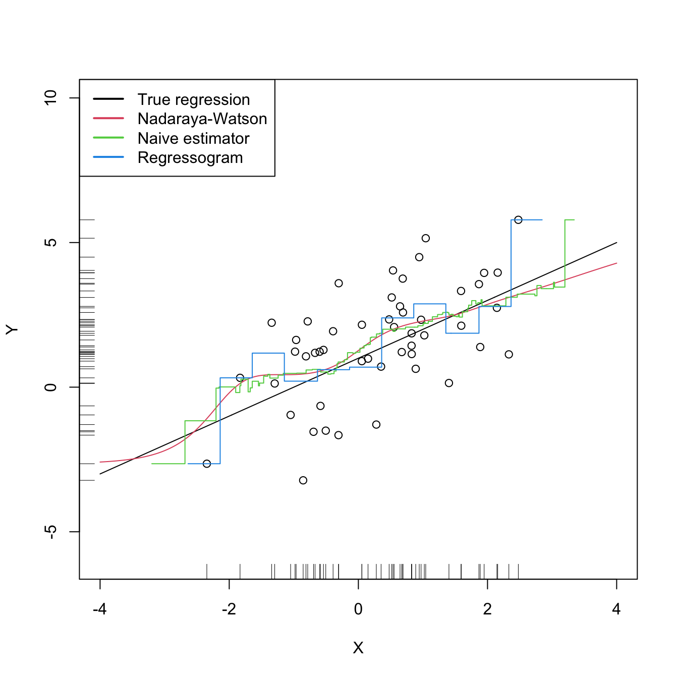
$The Nadaraya–Watson estimator, the naive regression estimator, and the regressogram. Notice that the naive regression estimator and the regressogram are not defined everywhere – only for those regions in which there are nearby observations of $X.$ All the estimators share the bandwidth $h=0.5,$ a fair comparison since the scaled uniform kernel, $\tilde K(z)=\frac{1}{2\sqrt{3}}1_{\{-\sqrt{3}<z<\sqrt{3}\}},$ is employed for the naive estimator. The regressogram employs $t_0=0.$ The regression setting is explained in Exercise 4.16.$

Figure 4.4: The Nadaraya–Watson estimator, the naive regression estimator, and the regressogram. Notice that the naive regression estimator and the regressogram are not defined everywhere – only for those regions in which there are nearby observations of $X.$ All the estimators share the bandwidth $h=0.5,$ a fair comparison since the scaled uniform kernel, $\tilde K(z)=\frac{1}{2\sqrt{3}}1_{\{-\sqrt{3}<z<\sqrt{3}\}},$ is employed for the naive estimator. The regressogram employs $t_0=0.$ The regression setting is explained in Exercise 4.16.

Exercise 4.16 Implement in R your own version of the naive regression estimator (4.27). It must be a function that takes as inputs:

a vector with the evaluation points $x,$
a sample $(X_1,Y_1),\ldots,(X_n,Y_n),$
a bandwidth $h,$

and that returns (4.27) evaluated for each $x.$ Test the implementation by estimating the regression function $m(x)=1+x$ for the regression model $Y=m(X)+\varepsilon,$ where $X\sim\mathcal{N}(0, 1)$ and $\varepsilon\sim\mathcal{N}(0,2)$ using $n=50$ observations. This is the setting used in Figure 4.4.

Exercise 4.17 Perform Exercise 4.16 by implementing in R the regressogram (4.28) instead of the naive regression estimator. The R function must now have an additional argument $t_0.$

4.5 Kernel regression estimation with `np`

The np package (Hayfield and Racine 2008) provides a complete framework for performing a more sophisticated nonparametric regression estimation for local constant and linear estimators, and for computing cross-validation bandwidths. The two workhorse functions for these tasks are np::npreg and np::npregbw, which illustrating the philosophy behind the np package: first, a suitable bandwidth for the nonparametric method is found (via np::npregbw) and stored in an rbandwidth object; then, a fitting function (np::npreg) is called on that rbandwidth object, which contains all the needed information.

# Data -- nonlinear trend
data(Auto, package = "ISLR")
X <- Auto$weight
Y <- Auto$mpg

# np::npregbw computes by default the least squares CV bandwidth associated
# with a local *constant* fit and admits a formula interface (to be exploited
# more in multivariate regression)
bw0 <- np::npregbw(formula = Y ~ X)
## Multistart 1 of 1 |Multistart 1 of 1 |Multistart 1 of 1 |Multistart 1 of 1 /Multistart 1 of 1 |Multistart 1 of 1 |                   

# The spinner can be omitted with
options(np.messages = FALSE)

# Multiple initial points can be employed for minimizing the CV function (for
# one predictor, defaults to 1) and avoiding local minima
bw0 <- np::npregbw(formula = Y ~ X, nmulti = 2)

# The "rbandwidth" object contains useful information, see ?np::npregbw for
# all the returned objects
bw0
## 
## Regression Data (392 observations, 1 variable(s)):
## 
##                      X
## Bandwidth(s): 110.1476
## 
## Regression Type: Local-Constant
## Bandwidth Selection Method: Least Squares Cross-Validation
## Formula: Y ~ X
## Bandwidth Type: Fixed
## Objective Function Value: 17.66388 (achieved on multistart 2)
## 
## Continuous Kernel Type: Second-Order Gaussian
## No. Continuous Explanatory Vars.: 1
head(bw0)
## $bw
## [1] 110.1476
## 
## $regtype
## [1] "lc"
## 
## $pregtype
## [1] "Local-Constant"
## 
## $method
## [1] "cv.ls"
## 
## $pmethod
## [1] "Least Squares Cross-Validation"
## 
## $fval
## [1] 17.66388
# Recall that the fit is very similar to h_CV

# Once the bandwidth is estimated, np::npreg can be directly called with the
# "rbandwidth" object (it encodes the regression to be made, the data, the kind
# of estimator considered, etc). The hard work happens in np::npregbw, not on
# np::npreg
kre0 <- np::npreg(bws = bw0)
kre0
## 
## Regression Data: 392 training points, in 1 variable(s)
##                      X
## Bandwidth(s): 110.1476
## 
## Kernel Regression Estimator: Local-Constant
## Bandwidth Type: Fixed
## 
## Continuous Kernel Type: Second-Order Gaussian
## No. Continuous Explanatory Vars.: 1

# Plot directly the fit via plot() -- it employs as evaluation points the
# (unsorted!) sample
plot(kre0, col = 2, type = "o")
points(X, Y)
rug(X, side = 1)
rug(Y, side = 2)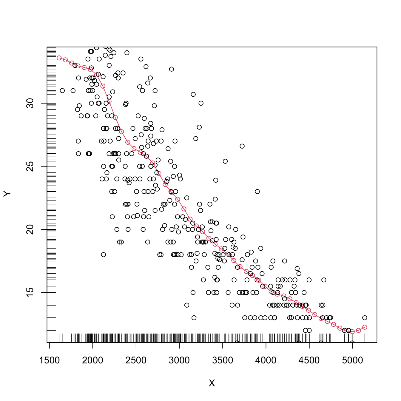

# lines(kre0$eval$X, kre0$mean, col = 3) # Not a good idea!

The type of local regression (local constant or local linear – no further local polynomial fits are implemented) is controlled by the argument regtype in np::npregbw: regtype = "ll" stands for “local linear” and regtype = "lc" for “local constant”.

# Local linear fit -- find first the CV bandwidth
bw1 <- np::npregbw(formula = Y ~ X, regtype = "ll")

# Fit
kre1 <- np::npreg(bws = bw1)

# Plot
plot(kre1, col = 2, type = "o")
points(X, Y)
rug(X, side = 1)
rug(Y, side = 2)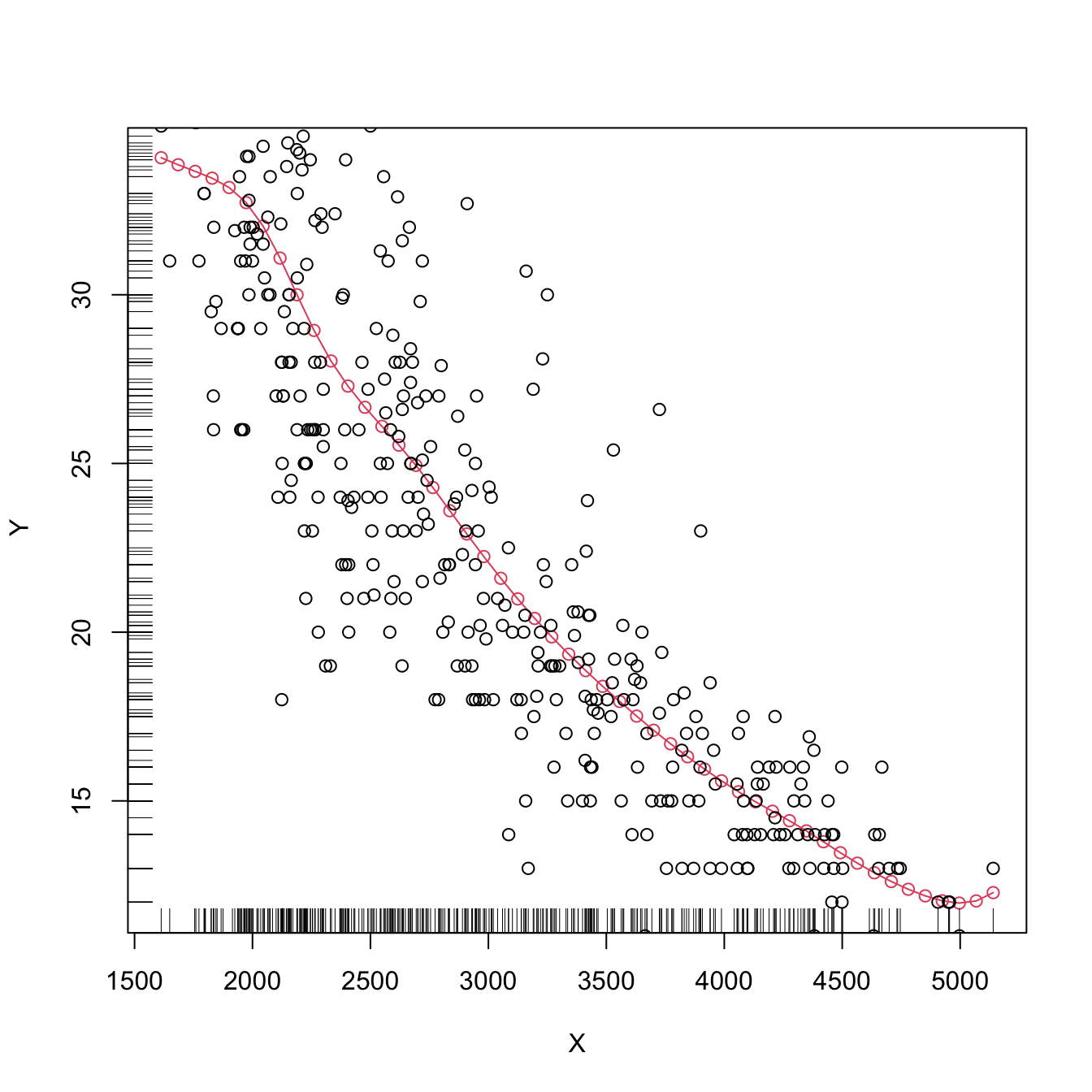

The following code shows in more detail the output object associated with np::npreg and how to change the evaluation points.

# Summary of the npregression object
summary(kre0)
##             Length Class      Mode     
## bw            1    -none-     numeric  
## bws          49    rbandwidth list     
## pregtype      1    -none-     character
## xnames        1    -none-     character
## ynames        1    -none-     character
## nobs          1    -none-     numeric  
## ndim          1    -none-     numeric  
## nord          1    -none-     numeric  
## nuno          1    -none-     numeric  
## ncon          1    -none-     numeric  
## pscaling      1    -none-     character
## ptype         1    -none-     character
## pckertype     1    -none-     character
## pukertype     1    -none-     character
## pokertype     1    -none-     character
## eval          1    data.frame list     
## mean        392    -none-     numeric  
## merr        392    -none-     numeric  
## grad          1    -none-     logical  
## gerr          1    -none-     logical  
## resid         1    -none-     logical  
## ntrain        1    -none-     numeric  
## trainiseval   1    -none-     logical  
## gradients     1    -none-     logical  
## residuals     1    -none-     logical  
## R2            1    -none-     numeric  
## MSE           1    -none-     numeric  
## MAE           1    -none-     numeric  
## MAPE          1    -none-     numeric  
## CORR          1    -none-     numeric  
## SIGN          1    -none-     numeric  
## nobs.omit     1    -none-     numeric  
## call          2    -none-     call

# Evaluation points (a data.frame) -- by default the sample (unsorted!)
head(kre0$eval)
##      X
## 1 3504
## 2 3693
## 3 3436
## 4 3433
## 5 3449
## 6 4341

# The estimation of the regression function at the evaluation points
head(kre0$mean)
## [1] 18.35364 17.10311 18.70083 18.71652 18.63411 14.23660

# The evaluation points can be changed using "exdat"
x_grid <- seq(1000, 5500, by = 5)
kre0 <- np::npreg(bws = bw0, exdat = x_grid)
kre1 <- np::npreg(bws = bw1, exdat = x_grid)

# Notice how $eval is a data.frame containing x_grid
head(kre0$eval)
##   x_grid
## 1   1000
## 2   1005
## 3   1010
## 4   1015
## 5   1020
## 6   1025

# This allows comparing estimators in a more transparent form
plot(X, Y)
lines(kre0$eval$x_grid, kre0$mean, col = 2)
lines(kre1$eval$x_grid, kre1$mean, col = 3)
rug(X, side = 1)
rug(Y, side = 2)
legend("top", legend = c("Nadaraya-Watson", "Local linear"),
       lwd = 2, col = 2:3)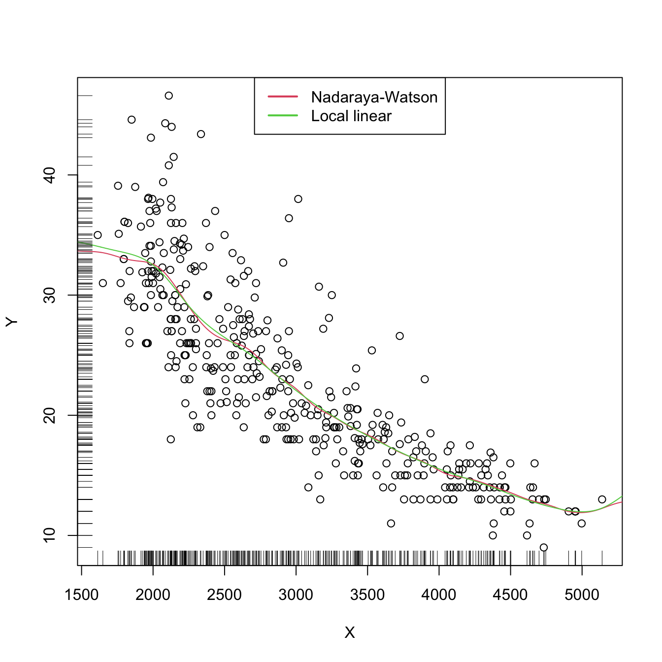

Now that we know how to effectively compute local constant and linear estimators, two insights with practical relevance become apparent:

The adequate bandwidths for the local linear estimator are usually larger than the adequate bandwidths for the local constant estimator. The reason is the extra flexibility that $\hat{m}(\cdot;1,h)$ has, which allows faster adaptation to variations in $m,$ whereas $\hat{m}(\cdot;0,h)$ can achieve this adaptability only by shrinking the neighborhood about $x$ by means of a smaller $h.$
Both estimators behave erratically at regions with low predictor’s density. This includes possible “holes” in the support of $X.$ In the absence of close data, the local constant estimator interpolates to a constant function that takes the value $Y_i$ of the closest $X_i$ to $x.$ However, the local linear estimator $\hat{m}(x;1,h)$ takes the value of the local linear regression $\hat{\beta}_{h,0}+\hat{\beta}_{h,1}(\cdot-x)$ that is determined by the two observations $(X_i,Y_i)$ with the closest $X_i$’s to $x.$ Hence, the local linear estimator extrapolates a line at regions with low $X$-density. This may have the undesirable consequence of yielding large spikes at these regions, which sharply contrasts with the “conservative behavior” of the local constant estimator.

The next two exercises are meant to evidence these two insights.

Exercise 4.18 Perform the following simulation study:

Simulate $n=200$ observations from the regression model $Y=m(X)+\varepsilon,$ where $X$ is distributed according to a nor1mix::MW.nm2, $m(x)=x\cos(x),$ and $\varepsilon+1\sim\mathrm{Exp}(1).$
Compute the CV bandwidths $\hat{h}_0$ and $\hat{h}_1$ for the local constant and linear estimators, respectively.
Repeat Steps 1–2 $M=1,000$ times. Trick: use the txtProgressBar and setTxtProgressBar functions to have an indication of the progress of the simulation.
Filter out large bandwidth outliers.

Then:

Compare graphically the two samples of $\hat{h}_0$ and $\hat{h}_1$. To do so, show in a plot the log-transformed kdes for the two samples and imitate the display given in Figure 4.5. Does there seem to be any type of stochastic dominance (check Section 6.2.1) between $\hat{h}_0$ and $\hat{h}_1$?
Repeat the simulation study for a different regression model and distributions for $X$ and $\varepsilon.$ Are the results consistent with the insights obtained before?

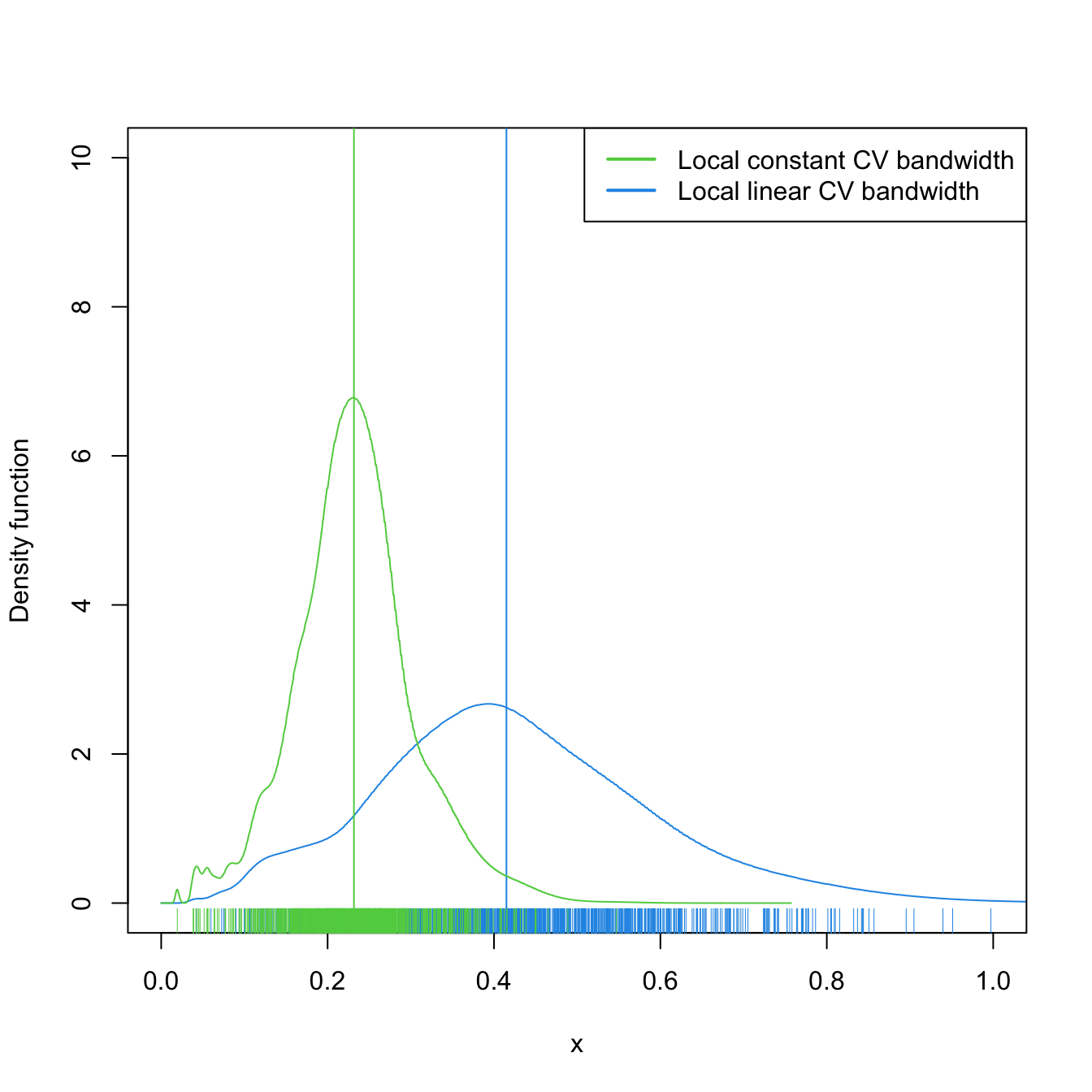
Estimated density for the local constant and local linear CV bandwidths, for the setting described in Exercise 4.18. The vertical bars denote the median CV bandwidths. Observe how local linear bandwidths tend to be larger than local constant ones.

Figure 4.5: Estimated density for the local constant and local linear CV bandwidths, for the setting described in Exercise 4.18. The vertical bars denote the median CV bandwidths. Observe how local linear bandwidths tend to be larger than local constant ones.

Exercise 4.19 Perform the following simulation study for each of the local constant and local linear estimators.

Plot the regression function $m(x)=x\cos(x).$
Simulate $n=100$ observations from the regression model $Y=m(X)+\varepsilon,$ where $\frac{1}{2}X$ is distributed according to a nor1mix::MW.nm7 and $\varepsilon\sim\mathcal{N}(0, 1).$
Compute the CV bandwidths and the associated local constant and linear fits.
Plot the fits as curves. Trick: adjust the transparency of each curve for better visualization.
Repeat Steps 2–4 $M=75$ times.

The two outputs should be similar to Figure 4.6. Increase the sample size to $n=200$ and consider $X$ such that $\frac{1}{4}X$ is distributed according to a nor1mix::MW.nm7. Comment on how well the estimators approximate the regression curve.

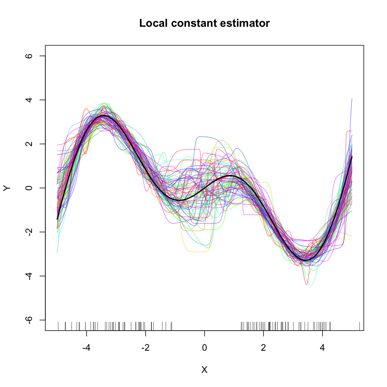
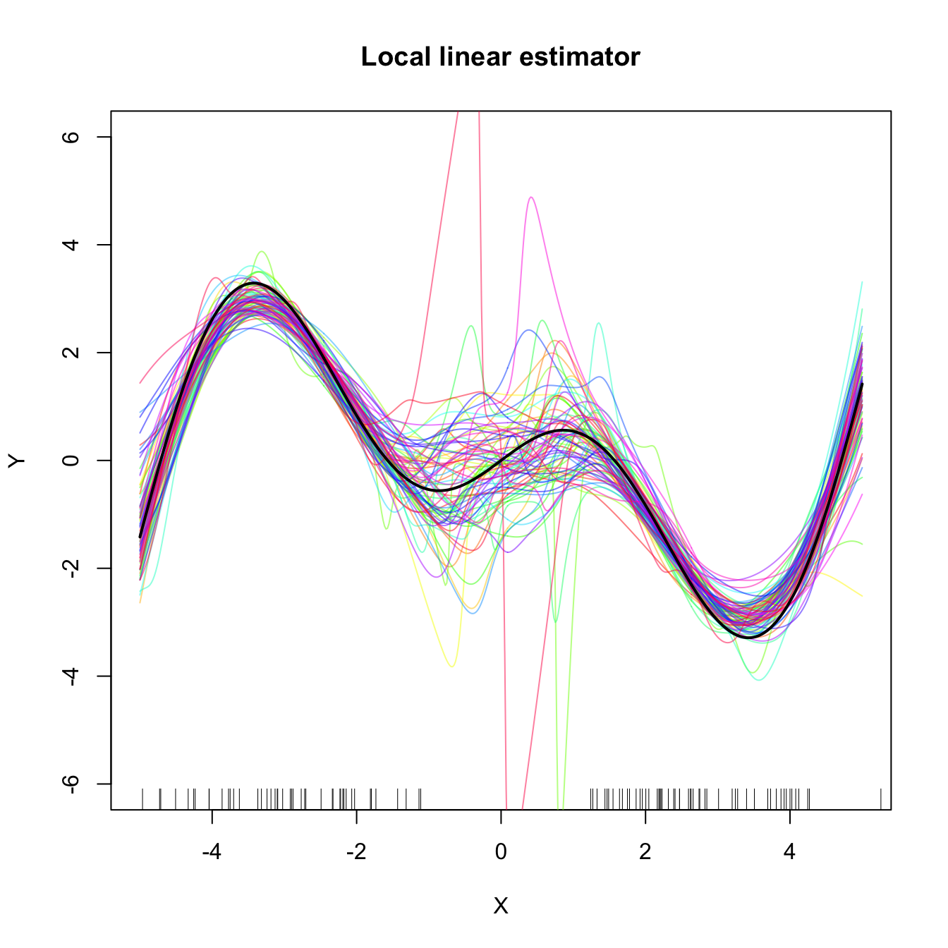
$Local constant and linear estimators of the regression function in the setting described in Exercise 4.19. The support of the predictor $X$ has a “hole”, which makes both estimators behave erratically at that region. The local linear estimator, driven by a local linear fit, may deviate more strongly from $m$ than the local constant.$ $Local constant and linear estimators of the regression function in the setting described in Exercise 4.19. The support of the predictor $X$ has a “hole”, which makes both estimators behave erratically at that region. The local linear estimator, driven by a local linear fit, may deviate more strongly from $m$ than the local constant.$

Figure 4.6: Local constant and linear estimators of the regression function in the setting described in Exercise 4.19. The support of the predictor $X$ has a “hole”, which makes both estimators behave erratically at that region. The local linear estimator, driven by a local linear fit, may deviate more strongly from $m$ than the local constant.

There are more sophisticated options for bandwidth selection available in np::npregbw. For example, the argument bwtype allows estimating data-driven variable bandwidths $\hat{h}(x)$ that depend on the evaluation point $x,$ rather than fixed bandwidths $\hat{h},$ as we have considered so far. Roughly speaking, these variable bandwidths are related to the variable bandwidth $\hat{h}_k(x)$ that is necessary to contain the $k$ nearest neighbors $X_1,\ldots,X_k$ of $x$ in the neighborhood $(x-\hat{h}_k(x),x+\hat{h}_k(x)).$ There is an interesting potential gain in employing variable bandwidths, as the local polynomial estimator can adapt the amount of smoothing according to the density of the predictor, therefore avoiding the aforementioned problems related to “holes” in the support of $X$ (see the code below). The extra flexibility of variable bandwidths changes the asymptotic properties of the local polynomial estimator. We do not investigate this approach in detail¹⁶⁵ but rather point to its implementation via np.

# Generate some data with bimodal density
set.seed(12345)
n <- 100
eps <- rnorm(2 * n, sd = 2)
m <- function(x) x^2 * sin(x)
X <- c(rnorm(n, mean = -2, sd = 0.5), rnorm(n, mean = 2, sd = 0.5))
Y <- m(X) + eps
x_grid <- seq(-10, 10, l = 500)

# Constant bandwidth
bwc <- np::npregbw(formula = Y ~ X, bwtype = "fixed",
                   regtype = "ll")
krec <- np::npreg(bwc, exdat = x_grid)

# Variable bandwidths
bwg <- np::npregbw(formula = Y ~ X, bwtype = "generalized_nn",
                   regtype = "ll")
kreg <- np::npreg(bwg, exdat = x_grid)
bwa <- np::npregbw(formula = Y ~ X, bwtype = "adaptive_nn",
                   regtype = "ll")
krea <- np::npreg(bwa, exdat = x_grid)

# Comparison
plot(X, Y)
rug(X, side = 1)
rug(Y, side = 2)
lines(x_grid, m(x_grid), col = 1)
lines(krec$eval$x_grid, krec$mean, col = 2)
lines(kreg$eval$x_grid, kreg$mean, col = 3)
lines(krea$eval$x_grid, krea$mean, col = 4)
legend("top", legend = c("True regression", "Fixed", "Generalized NN",
                         "Adaptive NN"),
       lwd = 2, col = 1:4)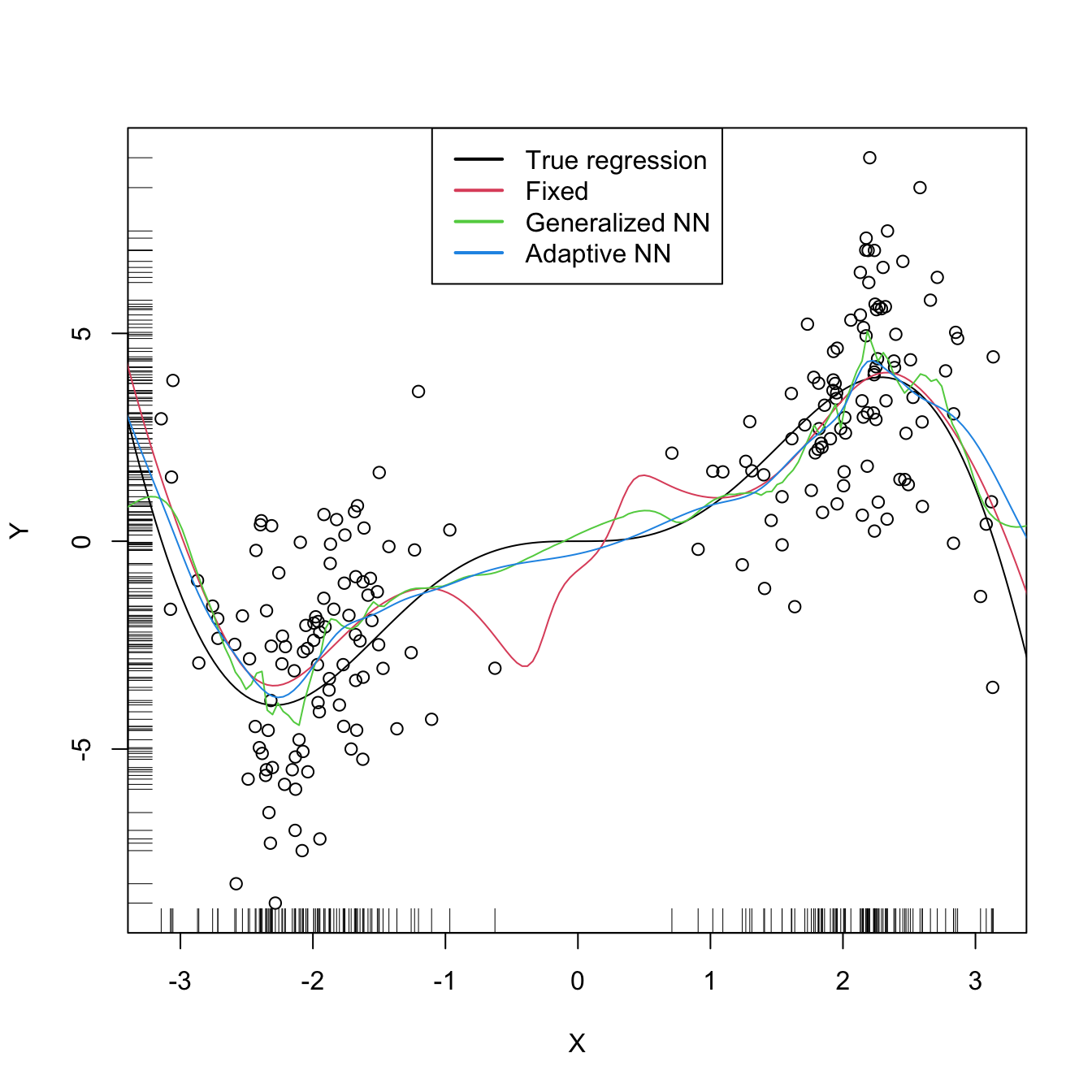

# Observe how the fixed bandwidth may yield a fit that produces serious
# artifacts in the low-density region. At that region the NN-based bandwidths
# expand to borrow strength from the points in the high-density regions,
# whereas in the high-density regions they shrink to adapt faster to the
# changes of the regression function

Exercise 4.20 Repeat Exercise 4.19 replacing Step 3 with:

Compute the variable bandwidths bwtype = "generalized_nn" and bwtype = "adaptive_nn" and the fits associated with them.

Then:

Describe the obtained results. Are they qualitatively different from those based on fixed bandwidths, given in Figure 4.6? Does any of the variable bandwidths seem to improve over fixed bandwidths?
What if you considered $n=200$ and $X$ is such that $\frac{1}{4}X$ is distributed according to a nor1mix::MW.nm7?
Construct an original scenario where you corroborate by simulations that the use of variable bandwidths (either "generalized_nn" or "adaptive_nn") improves the local regression fit significantly over fixed bandwidths.

Exercise 4.21 Consider the data(sunspots_births, package = "rotasym") dataset. Then:

Filter the dataset to account only for the 23rd solar cycle.
Inspect the graphical relation between dist_sun_disc (response) and log10(total_area + 1) (predictor).
Compute the CV bandwidth for the above regression, for the local linear estimator.
Compute and plot the local linear estimator using CV bandwidth. Comment on the fit.
Plot the local linear fits for the 23rd, 22nd, and 21st solar cycles. Do they have a similar pattern?
Randomly split the dataset for the 23rd cycle into a training sample ($80\%$) and testing sample ($20\%$). Repeat $10$ times these random splits. Then, compare the average mean square errors of the predictions by the local constant and local linear estimators with CV bandwidths. Comment on the results.

References

ESA. 1997. The Hipparcos and Tycho Catalogues. Vol. 1200. ESA SP. Noordwijk: ESA Publication Division. https://doi.org/https://www.cosmos.esa.int/web/hipparcos/catalogues.

Fan, J., and I. Gijbels. 1996. Local Polynomial Modelling and Its Applications. Vol. 66. Monographs on Statistics and Applied Probability. London: Chapman & Hall. https://doi.org/10.1201/9780203748725.

Hayfield, T., and J. S. Racine. 2008. “Nonparametric Econometrics: The np Package.” Journal of Statistical Software 27 (5): 1–32. https://doi.org/10.18637/jss.v027.i05.

Li, Q., and J. S. Racine. 2007. Nonparametric Econometrics. Princeton: Princeton University Press. https://press.princeton.edu/books/hardcover/9780691121611/nonparametric-econometrics.

Nadaraya, E. A. 1964. “On Estimating Regression.” Teoriya Veroyatnostei i Ee Primeneniya 9 (1): 157–59. https://doi.org/10.1137/1109020.

Ruppert, D., S. J. Sheather, and M. P. Wand. 1995. “An Effective Bandwidth Selector for Local Least Squares Regression.” Journal of the American Statistical Association 90 (432): 1257–70. https://doi.org/10.1080/01621459.1995.10476630.

Wand, M. P., and M. C. Jones. 1995. Kernel Smoothing. Vol. 60. Monographs on Statistics and Applied Probability. London: Chapman & Hall. https://doi.org/10.1201/b14876.

Watson, G. S. 1964. “Smooth Regression Analysis.” Sankhyā, Series A 26 (4): 359–72. https://www.jstor.org/stable/25049340.

For the sake of introducing the main concepts in kernel regression estimation. In Chapter 5 we will see more general situations with several predictors, possibly non-continuous.↩︎
Formally, the response $Y$ does not need to be continuous. We implicitly assume $Y$ is continuous to use (4.2) as a motivation for (4.5), but the subsequent derivations in the chapter are also valid for non-continuous responses.↩︎
Observe that in the third equality we use that $(X,Y)$ is continuous to motivate the construction of the estimator.↩︎
Notice that the estimator does not depend on $h_2;$ rather, it depends on $h_1,$ the bandwidth employed for smoothing $X.$↩︎
Termed due to the coetaneous proposals by Nadaraya (1964) and Watson (1964). Also known as the local-constant estimator for reasons explained next.↩︎
The change of the sum in the denominator from $\sum_{i=1}^n$ to $\sum_{j=1}^n$ is aimed to avoid confusions with the numerator.↩︎
Obviously, avoiding the spurious perfect fit attained with $\hat{m}(X_i):=Y_i,$ $i=1,\ldots,n.$↩︎
Here we employ $p$ to denote the order of the Taylor expansion (Theorem 1.11) and, correspondingly, the order of the associated polynomial fit. Do not confuse $p$ with the number of original predictors for explaining $Y$ – there is one predictor only, $X.$ However, with a local polynomial fit we expand this predictor to $p$ predictors based on $(X^1,X^2,\ldots,X^p).$↩︎
See (B.4) in Section B.1.1.↩︎
The rationale is simple: $(X_i,Y_i)$ should be more informative about $m(x)$ than $(X_j,Y_j)$ if $x$ and $X_i$ are closer than $x$ and $X_j.$↩︎
Recall that the entries of $\hat{\boldsymbol{\beta}}_h$ are estimating $\boldsymbol{\beta}=\left(m(x), m'(x),\frac{m''(x)}{2},\ldots,\frac{m^{(p)}(x)}{p!}\right)^\top,$ so we are indeed estimating $m(x)$ (first entry) and, in addition, its derivatives up to order $p.$↩︎
An alternative and useful view is that, by minimizing (4.10), we are fitting the linear model $\hat{m}_x(t):=\hat{\beta}_{h,0}+\hat{\beta}_{h,1}(t-x)+\cdots+\hat{\beta}_{h,p}(t-x)^p$ that is centered about $x.$ Then, we employ this model to predict $Y$ for $X=t=x,$ resulting in $\hat{\beta}_{h,0}.$↩︎
That is, the entries of $\mathbf{e}_i$ are all zero except for the $i$-th one, which is $1.$↩︎
Which is not a weighted mean in general, only if $p=0;$ see Exercise 4.6.↩︎
The lowess estimator, related to loess, is the one employed in R’s panel.smooth, which is the function in charge of displaying the smooth fits in lm and glm regression diagnostics (employing a prefixed and not data-driven smoothing span of $2/3$ – which makes it inevitably a bad choice for certain data patterns).↩︎
We do not address the analysis of the general case in which $p$ can be greater than one. The reader is referred to, for example, Theorem 3.1 in Fan and Gijbels (1996) for the full analysis.↩︎
In linear models, homoscedasticity is one of the key assumptions for performing inference (Section B.1.2).↩︎
Recall that these are the only assumptions made in the model so far. Compared with the ones linear models or generalized linear models make, they are extremely mild. Recall $Y$ is not assumed to be continuous.↩︎
This assumption requires certain smoothness of the regression function, allowing thus for Taylor expansions to be performed. This assumption is important in practice: $\hat{m}(\cdot;p,h)$ is infinitely differentiable if the considered kernels $K$ are so too.↩︎
It avoids the situation in which $Y$ is a degenerated random variable.↩︎
It avoids the degenerate situation in which $m$ is estimated at regions without observations of the predictors (such as holes in the support of $X$).↩︎
Meaning that there exists a positive lower bound for $f.$↩︎
Mild assumption inherited from the kde.↩︎
Key assumption for reducing the bias and variance of $\hat{m}(\cdot;p,h)$ simultaneously.↩︎
Recall that this makes perfect sense: low-density regions of $X$ imply less information available about $m.$↩︎
The same happened in the linear model with the error variance $\sigma^2.$↩︎
The variance of an unweighted mean is reduced by a factor $n^{-1}$ when $n$ observations are employed. To compute $\hat{m}(x;p,h),$ $n$ observations are used but in a weighted fashion that roughly amounts to considering $nh$ unweighted observations.↩︎
Since the variance increases as $\nu$ does, not as $p$ does.↩︎
$m(x)=c$ for all $x\in\mathbb{R}$ and given $c\in\mathbb{R}.$↩︎
$m(x)=ax+b$ for all $x\in\mathbb{R}$ and given $a,b\in\mathbb{R}.$↩︎
Estimating $m$ at regions with no data is an extrapolation problem. This kind of estimation makes better sense if a specific structure for $m$ is assumed (which is not done with a nonparametric estimate of $m$), so that this structure can determine the estimate of $m$ at the regions with no data.↩︎
The conditioning is on the sample of the predictor, as it is usually done in a regression setting. The reason why this conditioning is done is to avoid the analysis of the randomness of $X.$↩︎
In general, a polynomial fit of order $p+3$ can be considered, but we are restricting to $p=1.$ The motivation for this order is that it has to be able to estimate the $(p+1)$-th derivative of $m$ at $x,$ $m^{(p+1)}(x),$ with certain flexibility, and a polynomial fit of order $p+3$ would be able to do so by a quadratic polynomial.↩︎
Notice that the $n-5$ in the denominator appears because the degrees of freedom of the residuals in a polynomial fit of order $p+3$ is $n-p-4,$ and we are considering $p=1.$ Hence, $\hat{\sigma}_Q^2$ is an unbiased estimator of $\sigma_Q^2=\mathbb{V}\mathrm{ar}_Q[Y \mid X=x]=\mathbb{E}[(Y-m_Q(X))^2 \mid X=x].$↩︎
This is a slightly different adaptation from Fan and Gijbels (1996), where $\int\sigma^2(x)w_0(x)\,\mathrm{d}x$ is considered and therefore the estimate $\hat{\sigma}_Q^2\int w_0(x)\,\mathrm{d}x$ naturally follows. This weight $w_0,$ however, can be an indicator of the support of $X,$ which gives in that case the selector described here.↩︎
See Section 5.8 in Wand and Jones (1995) for a quick introduction.↩︎
Notice that this approach does not guarantee the continuity of the final estimate, but since the goal is on estimating the curvature this is not relevant.↩︎
So that, if $\sigma^2(x)$ is constant, $\int\sigma^2(x)\,\mathrm{d}x$ is finite because we integrate on a compact set.↩︎
In particular, the construction of block polynomial fits may be challenging to extend to $\mathbb{R}^p.$↩︎
Excluding colinear dispositions of the data and assuming that $n>p.$↩︎
In this case, when $h\to0,$ $\hat{m}_{-i}(X_i;p,h)\not\to Y_i$ because $(X_i,Y_i)$ does not belong to the sample employed for computing $\hat{m}_{-i}(\cdot;p,h).$ Notice that $\hat{m}_{-i}(X_j;p,h)\to Y_j$ when $h\to0$ if $j\neq i,$ but this is not problematic because in $\sum_{i=1}^n(Y_i-\hat{m}_{-i}(X_i;p,h))^2$ the leave-one-out estimate is different for each $i=1,\ldots,n.$↩︎
Indeed, for any other linear smoother of the response, the result will also hold.↩︎
For example, in astronomy, check Figure 3.2.17 in Vol. 1 in ESA (1997).↩︎
Equivalently, the naive density estimator $\hat{f}_\mathrm{N}(x;h)=\frac{1}{2nh}\sum_{i=1}^n1_{\{x-h<X_i<x+h\}}$ instead of the kde.↩︎
Observe that (4.27) is defined only for $x$ such that $|N(x;h)|>0.$ It is perfectly possible to have $|N(x;h)|=0$ in practice. This does not happen for non-compactly supported kernels, for which $N(x;h)=\mathbb{R}$ for any $x,$ $h,$ and sample arrangement.↩︎
The interested reader is referred to Chapter 14 in Li and Racine (2007) and references therein.↩︎

3 Kernel density estimation II

5 Kernel regression estimation II

4 Kernel regression estimation I

4.1 Kernel regression estimation

4.1.1 Nadaraya–Watson estimator

4.1.2 Local polynomial estimator

4.2 Asymptotic properties

4.3 Bandwidth selection

4.3.1 Plug-in rules

4.3.2 Cross-validation

4.4 Regressogram

4.5 Kernel regression estimation with np

References

4.5 Kernel regression estimation with `np`