5 Kernel regression estimation II

In Chapter 4 we studied the simplest situation for performing nonparametric estimation of the regression function: a single, continuous predictor \(X\) is available for explaining \(Y,\) a numerical response that is implicitly assumed to be continuous.¹⁶⁶ This served to introduce the main concepts without the additional technicalities associated with more complex predictors.

The purpose of this chapter is to extend nonparametric regression when

1. there are multiple predictors \(X_1,\ldots,X_p,\)
2. some predictors possibly are non-continuous, i.e., they are categorical or discrete, and
3. the response \(Y\) is not continuous.

We concentrate first on the first two points, as the third presents a change of paradigm from the kernel regression estimator studied in Chapter 4. See Section B.2 for a quick review on the relevant concepts of logistic regression used in this chapter.

5.1 Kernel regression with mixed multivariate data

5.1.1 Multivariate kernel regression

We start by addressing the first generalization:

How to extend the local polynomial estimator \(\hat{m}(\cdot;q,h)\,\)¹⁶⁷ to deal with \(p\) continuous predictors?

Although this can be done for \(q\geq0,\) we focus on the local constant and linear estimators (\(q=0,1\)) to avoid excessive technical complications.¹⁶⁸

The initial step is to state what the population object to be estimated is, which is now the function \(m:\mathbb{R}^p\longrightarrow\mathbb{R}\) given by¹⁶⁹

\[\begin{align} m(\mathbf{x}):=\mathbb{E}[Y\mid \mathbf{X}=\mathbf{x}]=\int yf_{Y\mid \mathbf{X}=\mathbf{x}}(y)\,\mathrm{d}y,\tag{5.1} \end{align}\]

where \(\mathbf{X}=(X_1,\ldots,X_p)^\top\) denotes the random vector of the predictors. Hence, despite having a form slightly different from (4.1), (5.1) is conceptually equal to (4.1). As a consequence, the density-based view¹⁷⁰ of \(m\) holds:

\[\begin{align} m(\mathbf{x})=\frac{\int y f(\mathbf{x},y)\,\mathrm{d}y}{f_\mathbf{X}(\mathbf{x})},\tag{5.2} \end{align}\]

where \(f\) is the joint density of \((\mathbf{X},Y)\) and \(f_\mathbf{X}\) is the marginal pdf of \(\mathbf{X}.\)

Therefore, given a sample \((\mathbf{X}_1,Y_1),\ldots,(\mathbf{X}_n,Y_n),\) we can estimate \(f\) and \(f_\mathbf{X},\) analogously to how we did in Section 4.1.1, by the kdes¹⁷¹

\[\begin{align} \hat{f}(\mathbf{x},y;\mathbf{H},h)&=\frac{1}{n}\sum_{i=1}^nK_{\mathbf{H}}(\mathbf{x}-\mathbf{X}_{i})K_{h}(y-Y_{i}),\tag{5.3}\\ \hat{f}_\mathbf{X}(\mathbf{x};\mathbf{H})&=\frac{1}{n}\sum_{i=1}^nK_{\mathbf{H}}(\mathbf{x}-\mathbf{X}_{i}).\tag{5.4} \end{align}\]

Plugging these estimators in (5.2), we readily obtain the Nadaraya–Watson estimator for multivariate predictors:

\[\begin{align} \hat{m}(\mathbf{x};0,\mathbf{H}):=\sum_{i=1}^n\frac{K_\mathbf{H}(\mathbf{x}-\mathbf{X}_i)}{\sum_{j=1}^nK_\mathbf{H}(\mathbf{x}-\mathbf{X}_j)}Y_i=\sum_{i=1}^nW^0_{i}(\mathbf{x})Y_i, \tag{5.5} \end{align}\]

where

\[\begin{align*} W^0_{i}(\mathbf{x}):=\frac{K_\mathbf{H}(\mathbf{x}-\mathbf{X}_i)}{\sum_{j=1}^nK_\mathbf{H}(\mathbf{x}-\mathbf{X}_j)}. \end{align*}\]

Exercise 5.1 Derive (5.5) by plugging (5.3) and (5.4) into (5.2).

Usually, to avoid a quick escalation of the number of smoothing bandwidths,¹⁷² it is customary to consider product kernels for smoothing \(\mathbf{X},\) that is, to consider a diagonal bandwidth \(\mathbf{H}=\mathrm{diag}(h_1^2,\ldots,h_p^2)=\mathrm{diag}(\mathbf{h}^2),\) which gives the estimator implemented by the np package:

\[\begin{align*} \hat{m}(\mathbf{x};0,\mathbf{h}):=\sum_{i=1}^nW^0_{i}(\mathbf{x})Y_i \end{align*}\]

where

\[\begin{align*} W^0_{i}(\mathbf{x})&=\frac{K_\mathbf{h}(\mathbf{x}-\mathbf{X}_i)}{\sum_{j=1}^nK_\mathbf{h}(\mathbf{x}-\mathbf{X}_j)},\\ K_\mathbf{h}(\mathbf{x}-\mathbf{X}_i)&=K_{h_1}(x_1-X_{i1})\times\stackrel{p}{\cdots}\times K_{h_p}(x_p-X_{ip}). \end{align*}\]

As in the univariate case, the Nadaraya–Watson estimate can be seen as a weighted average of \(Y_1,\ldots,Y_n\) by means of the weights \(\{W_i^0(\mathbf{x})\}_{i=1}^n.\) Therefore, the Nadaraya–Watson estimator is a local mean of \(Y_1,\ldots,Y_n\) about \(\mathbf{X}=\mathbf{x}.\)

The derivation of the local linear estimator involves slightly more complex arguments, but analogous to the extension of the linear model from univariate to multivariate predictors. Considering the first-order Taylor expansion

\[\begin{align*} m(\mathbf{X}_i)\approx m(\mathbf{x})+\mathrm{D}m(\mathbf{x})'(\mathbf{X}_i-\mathbf{x}), \end{align*}\]

instead of (4.7) it is possible to arrive at the analogue¹⁷³ of (4.10),

\[\begin{align*} \hat{\boldsymbol{\beta}}_\mathbf{h}:=\arg\min_{\boldsymbol{\beta}\in\mathbb{R}^{p+1}}\sum_{i=1}^n\left(Y_i-\boldsymbol{\beta}'(1,(\mathbf{X}_i-\mathbf{x})^\top)^\top\right)^2K_\mathbf{h}(\mathbf{x}-\mathbf{X}_i), \end{align*}\]

and then solve the problem in the exact same way but now considering the design matrix¹⁷⁴

\[\begin{align*} \mathbf{X}:=\begin{pmatrix} 1 & (\mathbf{X}_1-\mathbf{x})^\top\\ \vdots & \vdots\\ 1 & (\mathbf{X}_n-\mathbf{x})^\top\\ \end{pmatrix}_{n\times(p+1)} \end{align*}\]

and

\[\begin{align*} \mathbf{W}:=\mathrm{diag}(K_{\mathbf{h}}(\mathbf{X}_1-\mathbf{x}),\ldots, K_\mathbf{h}(\mathbf{X}_n-\mathbf{x})). \end{align*}\]

The estimate¹⁷⁵ for \(m(\mathbf{x})\) is therefore obtained from the solution of the weighted least squares problem

\[\begin{align*} \hat{\boldsymbol{\beta}}_{\mathbf{h}}&=\arg\min_{\boldsymbol{\beta}\in\mathbb{R}^{p+1}} (\mathbf{Y}-\mathbf{X}\boldsymbol{\beta})^\top\mathbf{W}(\mathbf{Y}-\mathbf{X}\boldsymbol{\beta})\\ &=(\mathbf{X}^\top\mathbf{W}\mathbf{X})^{-1}\mathbf{X}^\top\mathbf{W}\mathbf{Y} \end{align*}\]

as

\[\begin{align} \hat{m}(\mathbf{x};1,\mathbf{h}):=&\,\hat{\beta}_{\mathbf{h},0}\nonumber\\ =&\,\mathbf{e}_1'(\mathbf{X}^\top\mathbf{W}\mathbf{X})^{-1}\mathbf{X}^\top\mathbf{W}\mathbf{Y}\tag{5.6}\\ =&\,\sum_{i=1}^nW^1_{i}(\mathbf{x})Y_i,\nonumber \end{align}\]

where

\[\begin{align*} W^1_{i}(\mathbf{x}):=\mathbf{e}_1'(\mathbf{X}^\top\mathbf{W}\mathbf{X})^{-1}\mathbf{X}^\top\mathbf{W}\mathbf{e}_i. \end{align*}\]

Therefore, the local linear estimator is a weighted linear combination of the responses. Differently to the Nadaraya–Watson estimator, this linear combination is not a weighted mean in general, since the weights \(W^1_{i}(\mathbf{x})\) can be negative despite \(\sum_{i=1}^nW_i^1(\mathbf{x})=1.\)

Exercise 5.2 Implement an R function to compute \(\hat{m}(\mathbf{x};1,h)\) for an arbitrary dimension \(p.\) The function must receive as arguments the sample \((\mathbf{X}_1,Y_1),\ldots,(\mathbf{X}_n,Y_n),\) the bandwidth vector \(\mathbf{h},\) and a collection of evaluation points \(\mathbf{x}.\) Implement the function by computing the design matrix \(\mathbf{X},\) the weight matrix \(\mathbf{W},\) the vector of responses \(\mathbf{Y},\) and then applying (5.6). Test the implementation in the example below and with other synthetic examples.

The following code performs the local regression estimators with two predictors and exemplifies how the use of np::npregbw and np::npreg is analogous in this bivariate case.

# Sample data from a bivariate regression
n <- 300
set.seed(123456)
X <- mvtnorm::rmvnorm(n = n, mean = c(0, 0),
                      sigma = matrix(c(2, 0.5, 0.5, 1.5), nrow = 2, ncol = 2))
m <- function(x) 0.5 * (x[, 1]^2 + x[, 2]^2)
epsilon <- rnorm(n)
Y <- m(x = X) + epsilon

# Plot sample and regression function
rgl::plot3d(x = X[, 1], y = X[, 2], z = Y, xlim = c(-3, 3), ylim = c(-3, 3),
            zlim = c(-4, 10), xlab = "X1", ylab = "X2", zlab = "Y")
lx <- ly <- 50
x_grid <- seq(-3, 3, l = lx)
y_grid <- seq(-3, 3, l = ly)
xy_grid <- as.matrix(expand.grid(x_grid, y_grid))
rgl::surface3d(x = x_grid, y = y_grid,
               z = matrix(m(xy_grid), nrow = lx, ncol = ly),
               col = "lightblue", alpha = 1, lit = FALSE)

# Local constant fit

# An alternative for calling np::npregbw without formula
bw0 <- np::npregbw(xdat = X, ydat = Y, regtype = "lc")
kre0 <- np::npreg(bws = bw0, exdat = xy_grid) # Evaluation grid is now a matrix
rgl::surface3d(x = x_grid, y = y_grid,
               z = matrix(kre0$mean, nrow = lx, ncol = ly),
               col = "red", alpha = 0.25, lit = FALSE)

# Local linear fit
bw1 <- np::npregbw(xdat = X, ydat = Y, regtype = "ll")
kre1 <- np::npreg(bws = bw1, exdat = xy_grid)
rgl::surface3d(x = x_grid, y = y_grid,
               z = matrix(kre1$mean, nrow = lx, ncol = ly),
               col = "green", alpha = 0.25, lit = FALSE)
rgl::rglwidget()

Let’s see an application of multivariate kernel regression for the wine.csv dataset. The objective in this dataset is to explain and predict the quality of a vintage, measured as its Price, by means of predictors associated with the vintage.

# Load the wine dataset
wine <- read.table(file = "datasets/wine.csv", header = TRUE, sep = ",")

# Bandwidth by CV for local linear estimator -- a product kernel with
# 4 bandwidths
# Employs 4 random starts for minimizing the CV surface
bw_wine <- np::npregbw(formula = Price ~ Age + WinterRain + AGST +
                         HarvestRain, data = wine, regtype = "ll")
bw_wine
## 
## Regression Data (27 observations, 4 variable(s)):
## 
##                   Age WinterRain      AGST HarvestRain
## Bandwidth(s): 4050865  395622046 0.8725243     106.508
## 
## Regression Type: Local-Linear
## Bandwidth Selection Method: Least Squares Cross-Validation
## Formula: Price ~ Age + WinterRain + AGST + HarvestRain
## Bandwidth Type: Fixed
## Objective Function Value: 0.0873955 (achieved on multistart 3)
## 
## Continuous Kernel Type: Second-Order Gaussian
## No. Continuous Explanatory Vars.: 4

# Regression
fit_wine <- np::npreg(bw_wine)
summary(fit_wine)
## 
## Regression Data: 27 training points, in 4 variable(s)
##                   Age WinterRain      AGST HarvestRain
## Bandwidth(s): 4050865  395622046 0.8725243     106.508
## 
## Kernel Regression Estimator: Local-Linear
## Bandwidth Type: Fixed
## Residual standard error: 0.2079692
## R-squared: 0.8889648
## 
## Continuous Kernel Type: Second-Order Gaussian
## No. Continuous Explanatory Vars.: 4

# Plot the "marginal effects of each predictor" on the response
plot(fit_wine)

# Observe that the massive bandwidths for Age and WinterRain imply that the
# variables enter in a linear fashion in the local linear fit (i.e., the
# smoothing is so large that a global linear model is fit for each predictor).

# These marginal effects are the p profiles of the estimated regression surface
# \hat{m}(x_1, ..., x_p) that are obtained by fixing the predictors to each of
# their median values. For example, the profile for Age is the curve
# \hat{m}(x, median_WinterRain, median_AGST, median_HarvestRain). The medians
# are:
apply(wine[c("Age", "WinterRain", "AGST", "HarvestRain")], 2, median)
##         Age  WinterRain        AGST HarvestRain 
##     16.0000    600.0000     16.4167    123.0000

# Therefore, conditionally on the median values of the predictors:
# - Age is positively related to Price (essentially linearly)
# - WinterRain is positively related to Price (essentially linearly)
# - AGST is positively related to Price with what it seems like a
#   quadratic pattern
# - HarvestRain is negatively related to Price (with a linear-like relation)

The many options for the plot method for np::npreg can be seen at ?np::npplot. We illustrate as follows some of them with a view to enhancing the interpretability of the marginal effects.

# The argument "xq" controls the conditioning quantile of the predictors, by
# default the median (xq = 0.5). But xq can be a vector of p quantiles, for
# example (0.25, 0.5, 0.25, 0.75) for (Age, WinterRain, AGST, HarvestRain)
plot(fit_wine, xq = c(0.25, 0.5, 0.25, 0.75))

# With "plot.behavior = data" the plot function returns a list with the data
# for performing the plots
res <- plot(fit_wine, xq = 0.5, plot.behavior = "data")
str(res, 1)
## List of 4
##  $ r1:List of 35
##   ..- attr(*, "class")= chr "npregression"
##  $ r2:List of 35
##   ..- attr(*, "class")= chr "npregression"
##  $ r3:List of 35
##   ..- attr(*, "class")= chr "npregression"
##  $ r4:List of 35
##   ..- attr(*, "class")= chr "npregression"

# Plot the marginal effect of AGST ($r3) alone
head(res$r3$eval) # All the predictors are constant (medians, except AGST)
##   V1  V2       V3  V4
## 1 16 600 14.98330 123
## 2 16 600 15.03772 123
## 3 16 600 15.09214 123
## 4 16 600 15.14657 123
## 5 16 600 15.20099 123
## 6 16 600 15.25541 123
plot(res$r3$eval$V3, res$r3$mean, type = "l", xlab = "AGST",
     ylab = "Marginal effect")

# Plot the marginal effects of AGST for varying quantiles in the rest of
# predictors (all with the same quantile)
tau <- seq(0.1, 0.9, by = 0.1)
res <- plot(fit_wine, xq = tau[1], plot.behavior = "data")
col <- viridis::viridis(length(tau))
plot(res$r3$eval$V3, res$r3$mean, type = "l", xlab = "AGST",
     ylab = "Marginal effect", col = col[1], ylim = c(6, 9),
     main = "Marginal effects of AGST for varying quantiles in the predictors")
for (i in 2:length(tau)) {
  res <- plot(fit_wine, xq = tau[i], plot.behavior = "data")
  lines(res$r3$eval$V3, res$r3$mean, col = col[i])
}
legend("topleft", legend = latex2exp::TeX(paste0("$\\tau =", tau, "$")),
       col = col, lwd = 2)

# These quantiles are
apply(wine[c("Age", "WinterRain", "HarvestRain")], 2, quantile, prob = tau)
##      Age WinterRain HarvestRain
## 10%  5.6      419.2        65.2
## 20%  8.2      508.8        86.2
## 30% 10.8      567.8        94.6
## 40% 13.4      576.2       114.4
## 50% 16.0      600.0       123.0
## 60% 18.6      609.2       156.8
## 70% 21.2      691.4       173.6
## 80% 23.8      716.4       187.0
## 90% 26.8      785.4       255.0

For the predictor \(X_1\), the marginal effect computed by np::npplot is the profile curve described by the function \[\begin{align} x_1\mapsto \hat{m}(x_1,X_{(\lfloor \alpha_2n \rfloor)2},\ldots,X_{(\lfloor \alpha_p n \rfloor)p};q,\mathbf{h}), \tag{5.7} \end{align}\] with \(\alpha_1,\ldots,\alpha_p\in[0,1]\) (by default, \(\alpha_2=\cdots=\alpha_p=0.5\)). Above, \(X_{(\lfloor \alpha_{j}n \rfloor)j}\) is the \(\alpha_j\)-quantile of the sample \(\{X_{1j},\ldots,X_{nj}\},\) for \(X_j,\) \(j=2,\ldots,p.\) The plots constructed with (5.7) are related to the so-called Individual Conditional Expectation (ICE) plots,¹⁷⁶ which are generally applicable to have interpretability of any fitted regression model \(\hat{m}.\) The function (5.7) can be seen as the estimator of the population profile function \[\begin{align} x_1\mapsto m(x_1,X_{2;\alpha_2},\ldots,X_{p;\alpha_p};q,\mathbf{h}), \tag{5.8} \end{align}\] where \(X_{j;\alpha_j}\) is the \(\alpha_j\)-quantile of \(X_j,\) \(j=2,\ldots,p.\) ICE plots are related with the so-called Partial Dependence (PD) plots,¹⁷⁷ which display the estimated marginal regression function \[\begin{align} \hat{m}_1(x_1;q,\mathbf{h}):=\frac{1}{n}\sum_{i=1}^n \hat{m}(x_1,X_{i2},\ldots,X_{ip};q,\mathbf{h}) \tag{5.9} \end{align}\] that estimates its population version \[\begin{align} m_1(x_1):=\mathbb{E}[Y \mid X_1=x_1]=\mathbb{E}[m(\mathbf{X}) \mid X_1=x_1]. \tag{5.10} \end{align}\]

Exercise 5.3 Dive into the similarities and differences between (5.7) and (5.9), and (5.8) and (5.10). For that, consider the regression model \[ Y=\beta_0+\beta_1X_1^2+\beta_2X_2+\beta_3X_3+\varepsilon, \quad X_1,X_2,\varepsilon\sim \mathcal{N}(0,1), \quad X_3\sim \mathrm{Exp}(1), \] with independent predictors and errors. Simulate \(M=10\) samples of size \(n=100\) from this model with \(\beta_j\neq0\) for \(j=0,1,2,3\) set at your disposal. Then, for each predictor:

1. Derive the population curves (5.8) and (5.10) and plot them. Discuss the similarities and differences between both curves.
2. Overlay the estimators (5.7) and (5.9) on top, using cross-validation bandwidths. Discuss the approximation to the population curves for different sample sizes \(n.\)
3. Construct a nonlinear regression model featuring dependent predictors where the difference between (5.8) and (5.10) is more pronounced. If needed, approximate these curves using Monte Carlo.

Condition on the median values of the other predictors.

The summary of np::npreg returns an \(R^2.\) This statistic is defined as

\[\begin{align*} R^2:=\frac{(\sum_{i=1}^n(Y_i-\bar{Y})(\hat{Y}_i-\bar{Y}))^2}{(\sum_{i=1}^n(Y_i-\bar{Y})^2)(\sum_{i=1}^n(\hat{Y}_i-\bar{Y})^2)} \end{align*}\]

and is neither the squared correlation coefficient between \(Y_1,\ldots,Y_n\) and \(\hat{Y}_1,\ldots,\hat{Y}_n\,\)¹⁷⁸ \(\!\!^,\)¹⁷⁹ nor “the percentage of variance explained” by the model – this interpretation makes sense within the linear model context only. It is however a quantity in \([0,1]\) that attains \(R^2=1\) whenever the fit is perfect (zero variability about the curve), so it can give an idea of how explicative the estimated regression function is.

5.1.2 Kernel regression with mixed data

Non-continuous predictors can also be taken into account in nonparametric regression. The key to do so is an adequate definition of a suitable kernel function for any random variable \(X,\) not just continuous. Therefore, we need to find

a positive function that is a pdf¹⁸⁰ on the support of \(X\) and that allows assigning more weight to observations of the random variable that are close to a given point.

If such kernel is adequately defined, then it can be readily employed in the weights of the linear combinations that form \(\hat{m}(\cdot;q,\mathbf{h}).\)

We analyze next the two main possibilities for non-continuous variables:

• Categorical or unordered discrete variables. For example, iris$Species and Auto$origin are categorical variables in which ordering does not make any sense. Categorical variables are specified in base R by factor. Due to the lack of ordering, the basic mathematical operation behind a kernel, a distance computation,¹⁸¹ is delicate. This motivates the Aitchison and Aitken (1976) kernel.

  Assume that the categorical random variable \(X_d\) has \(u_d\) different levels. These levels can be represented as \(U_d:=\{0,1,\ldots,u_d-1\}.\) For \(x_d,X_d\in U_d,\) the Aitchison and Aitken (1976) unordered discrete kernel is

  \[\begin{align*} l_u(x_d,X_d;\lambda):=\begin{cases} 1-\lambda,&\text{ if }x_d=X_d,\\ \frac{\lambda}{u_d-1},&\text{ if }x_d\neq X_d, \end{cases} \end{align*}\]

  where \(\lambda\in[0,(u_d-1)/u_d]\) is the bandwidth. Observe that this kernel is constant if \(x_d\neq X_d\): since the levels of the variable are unordered, there is no sense of proximity between them. In other words, the kernel only distinguishes if two levels are equal or not to assign weight. If \(\lambda=0,\) then no weight is assigned if \(x_d\neq X_d\) and no information is borrowed from different levels; hence, nonparametrically regressing \(Y\) onto \(X_d\) is equivalent to doing \(u_d\) separate nonparametric regressions. If \(\lambda=(u_d-1)/u_d,\) then all levels are assigned the same weight, regardless of \(x_d;\) hence, \(X_d\) is irrelevant for explaining \(Y.\)

• Ordinal or ordered discrete variables. For example, wine$Year and Auto$cylinders are discrete variables with clear orders, but they are not continuous. These variables are specified by ordered (an ordered factor in base R). Despite the existence of an ordering, the possible distances between the observations of these variables are discrete.

  Assume that the ordered discrete random variable \(X_d\) takes values in a set \(O_d.\) For \(x_d,X_d\in O_d,\) a possible (Li and Racine 2007) ordered discrete kernel is¹⁸²

  \[\begin{align*} l_o(x_d,X_d;\eta):=\eta^{|x_d-X_d|}, \end{align*}\]

  where \(\eta\in[0,1]\) is the bandwidth.¹⁸³ If \(\eta=0,1,\) then

  \[\begin{align*} l_o(x_d,X_d;0)=\begin{cases}0,&x_d\neq X_d,\\1,&x_d=X_d,\end{cases}\quad l_o(x_d,X_d;1)=1. \end{align*}\]

  Hence, if \(\eta=0,\) nonparametrically regressing \(Y\) onto \(X_d\) is equivalent to doing separate nonparametric regressions for each of the levels of \(X_d.\) If \(\eta=1,\) \(X_d\) is irrelevant for explaining \(Y.\)

Exercise 5.4 Show that, for any \(X_d\in U_d\) and any \(\lambda\in[0,(u_d-1)/u_d],\) the kernel \(x\mapsto l_u(x,X_d;\lambda)\) “integrates” one over \(U_d.\)

Once we have defined the suitable kernels for ordered and unordered discrete variables, we can “aggregate” information from nearby observations of mixed data. Assume that, among the \(p=p_c+p_u+p_o\) predictors, the first \(p_c\) are continuous, the next \(p_u\) are discrete unordered (or categorical), and the last \(p_o\) are discrete ordered (or ordinal). The Nadaraya–Watson for mixed multivariate data is defined as

\[\begin{align} \hat{m}(\mathbf{x};0,(\mathbf{h}_c,\boldsymbol{\lambda}_u,\boldsymbol{\eta}_o)):=\sum_{i=1}^nW^0_{i}(\mathbf{x})Y_i,\tag{5.11} \end{align}\]

with the weights of the estimator being

\[\begin{align} W^0_{i}(\mathbf{x})=\frac{L_\Pi(\mathbf{x},\mathbf{X}_i)}{\sum_{j=1}^nL_\Pi(\mathbf{x},\mathbf{X}_j)}.\tag{5.12} \end{align}\]

The weights are based on the mixed product kernel

\[\begin{align*} L_\Pi(\mathbf{x},\mathbf{X}_i):=&\,\prod_{j=1}^{p_c}K_{h_j}(x_j-X_{ij})\prod_{k=1}^{p_u}l_u(x_k,X_{ik};\lambda_k)\prod_{\ell=1}^{p_o}l_o(x_\ell,X_{i\ell};\eta_\ell), \end{align*}\]

which features the vectors of bandwidths \(\mathbf{h}_c=(h_1,\ldots,h_{p_c})^\top,\) \(\boldsymbol{\lambda}_u=(\lambda_1,\ldots,\lambda_{p_u})^\top,\) and \(\boldsymbol{\eta}_o=(\eta_1,\ldots,\eta_{p_o})^\top\) for each cluster of equal-type predictors.

The adaptation of the local linear estimator is conceptually similar to that of the local constant, but it is more cumbersome as linear approximations make sense for quantitative variables, but not for unordered predictors. Therefore, the local linear estimator with mixed predictors is skipped in this book.

The np package employs a variation of the previous kernels and implements the local constant and linear estimators for mixed multivariate data.

# Bandwidth by CV for local constant estimator
# Recall that Species is a factor!
bw_iris <- np::npregbw(formula = Petal.Length ~ Sepal.Width + Species,
                       data = iris)
bw_iris
## 
## Regression Data (150 observations, 2 variable(s)):
## 
##               Sepal.Width      Species
## Bandwidth(s):   0.1900844 1.557114e-07
## 
## Regression Type: Local-Constant
## Bandwidth Selection Method: Least Squares Cross-Validation
## Formula: Petal.Length ~ Sepal.Width + Species
## Bandwidth Type: Fixed
## Objective Function Value: 0.15642 (achieved on multistart 2)
## 
## Continuous Kernel Type: Second-Order Gaussian
## No. Continuous Explanatory Vars.: 1
## 
## Unordered Categorical Kernel Type: Aitchison and Aitken
## No. Unordered Categorical Explanatory Vars.: 1
# Product kernel with 2 bandwidths

# Regression
fit_iris <- np::npreg(bw_iris)
summary(fit_iris)
## 
## Regression Data: 150 training points, in 2 variable(s)
##               Sepal.Width      Species
## Bandwidth(s):   0.1900844 1.557114e-07
## 
## Kernel Regression Estimator: Local-Constant
## Bandwidth Type: Fixed
## Residual standard error: 0.3715518
## R-squared: 0.9554129
## 
## Continuous Kernel Type: Second-Order Gaussian
## No. Continuous Explanatory Vars.: 1
## 
## Unordered Categorical Kernel Type: Aitchison and Aitken
## No. Unordered Categorical Explanatory Vars.: 1

# Plot marginal effects (for quantile 0.5) of each predictor on the response
par(mfrow = c(1, 2))
plot(fit_iris, plot.par.mfrow = FALSE)

# Options for the plot method for np::npreg can be seen at ?np::npplot

# Plot marginal effects (for quantile 0.9) of each predictor on the response
par(mfrow = c(1, 2))
plot(fit_iris, xq = 0.9, plot.par.mfrow = FALSE)

The following is an example from ?np::npreg: the modeling of the GDP growth of a country from economic indicators. The predictors contain a mix of unordered, ordered, and continuous variables.

# Load data
data(oecdpanel, package = "np")

# Bandwidth by CV for local constant -- use only two starts to reduce the
# computation time
bw_OECD <- np::npregbw(formula = growth ~ oecd + ordered(year) +
                         initgdp + popgro + inv + humancap, data = oecdpanel,
                       regtype = "lc", nmulti = 2)
bw_OECD
## 
## Regression Data (616 observations, 6 variable(s)):
## 
##                     oecd ordered(year)   initgdp    popgro       inv  humancap
## Bandwidth(s): 0.01206227     0.8794879 0.3329921 0.0597245 0.1594767 0.9407897
## 
## Regression Type: Local-Constant
## Bandwidth Selection Method: Least Squares Cross-Validation
## Formula: growth ~ oecd + ordered(year) + initgdp + popgro + inv + humancap
## Bandwidth Type: Fixed
## Objective Function Value: 0.0006358702 (achieved on multistart 2)
## 
## Continuous Kernel Type: Second-Order Gaussian
## No. Continuous Explanatory Vars.: 4
## 
## Unordered Categorical Kernel Type: Aitchison and Aitken
## No. Unordered Categorical Explanatory Vars.: 1
## 
## Ordered Categorical Kernel Type: Li and Racine
## No. Ordered Categorical Explanatory Vars.: 1

# Recall that ordered(year) is doing an in-formula transformation of year,
# which is *not* codified as an ordered factor in the oecdpanel dataset
# Therefore, if ordered() was not present, year would have been treated
# as continuous, as illustrated below
np::npregbw(formula = growth ~ oecd + year + initgdp + popgro +
              inv + humancap, data = oecdpanel, regtype = "lc", nmulti = 2)
## 
## Regression Data (616 observations, 6 variable(s)):
## 
##                     oecd     year   initgdp     popgro       inv  humancap
## Bandwidth(s): 0.01644512 7.481232 0.3486883 0.05860077 0.1639842 0.8371089
## 
## Regression Type: Local-Constant
## Bandwidth Selection Method: Least Squares Cross-Validation
## Formula: growth ~ oecd + year + initgdp + popgro + inv + humancap
## Bandwidth Type: Fixed
## Objective Function Value: 0.0006338394 (achieved on multistart 1)
## 
## Continuous Kernel Type: Second-Order Gaussian
## No. Continuous Explanatory Vars.: 5
## 
## Unordered Categorical Kernel Type: Aitchison and Aitken
## No. Unordered Categorical Explanatory Vars.: 1

# A cleaner approach to avoid doing the in-formula transformation, which
# may be problematic when using predict() or np_pred_CI(), is to directly
# change in the dataset the nature of the factor/ordered variables that are
# not codified as such. For example:
oecdpanel$year <- ordered(oecdpanel$year)
bw_OECD <- np::npregbw(formula = growth ~ oecd + year + initgdp + popgro +
                         inv + humancap, data = oecdpanel,
                       regtype = "lc", nmulti = 2)
bw_OECD
## 
## Regression Data (616 observations, 6 variable(s)):
## 
##                     oecd      year  initgdp     popgro       inv  humancap
## Bandwidth(s): 0.01206276 0.8794881 0.332989 0.05972475 0.1594737 0.9408023
## 
## Regression Type: Local-Constant
## Bandwidth Selection Method: Least Squares Cross-Validation
## Formula: growth ~ oecd + year + initgdp + popgro + inv + humancap
## Bandwidth Type: Fixed
## Objective Function Value: 0.0006358702 (achieved on multistart 2)
## 
## Continuous Kernel Type: Second-Order Gaussian
## No. Continuous Explanatory Vars.: 4
## 
## Unordered Categorical Kernel Type: Aitchison and Aitken
## No. Unordered Categorical Explanatory Vars.: 1
## 
## Ordered Categorical Kernel Type: Li and Racine
## No. Ordered Categorical Explanatory Vars.: 1

# Regression
fit_OECD <- np::npreg(bw_OECD)
summary(fit_OECD)
## 
## Regression Data: 616 training points, in 6 variable(s)
##                     oecd      year  initgdp     popgro       inv  humancap
## Bandwidth(s): 0.01206276 0.8794881 0.332989 0.05972475 0.1594737 0.9408023
## 
## Kernel Regression Estimator: Local-Constant
## Bandwidth Type: Fixed
## Residual standard error: 0.01737053
## R-squared: 0.7143326
## 
## Continuous Kernel Type: Second-Order Gaussian
## No. Continuous Explanatory Vars.: 4
## 
## Unordered Categorical Kernel Type: Aitchison and Aitken
## No. Unordered Categorical Explanatory Vars.: 1
## 
## Ordered Categorical Kernel Type: Li and Racine
## No. Ordered Categorical Explanatory Vars.: 1

# Plot marginal effects of each predictor on the response
par(mfrow = c(2, 3))
plot(fit_OECD, plot.par.mfrow = FALSE)

Exercise 5.5 Obtain the local constant estimator of the regression of mpg on cylinders (ordered discrete), horsepower, weight, and origin in the data(Auto, package = "ISLR") dataset. Summarize the model and plot the marginal effects of each predictor on the response (for the quantile \(0.5\)).

5.2 Bandwidth selection

Cross-validatory bandwidth selection, as studied in Section 4.3, extends neatly to the mixed multivariate case. For the fully continuous case, the least-squares cross validation selector is defined as

\[\begin{align*} \mathrm{CV}(\mathbf{h})&:=\frac{1}{n}\sum_{i=1}^n(Y_i-\hat{m}_{-i}(\mathbf{X}_i;q,\mathbf{h}))^2,\\ \hat{\mathbf{h}}_\mathrm{CV}&:=\arg\min_{h_1,\ldots,h_p>0}\mathrm{CV}(\mathbf{h}). \end{align*}\]

The cross-validation objective function becomes more challenging to minimize as \(p\) grows. This is the reason why employing several starting values for optimizing it (as np does) is advisable.

The mixed case is defined in a completely analogous manner by just replacing continuous kernels \(K_h(\cdot)\) with categorical \(l_u(\cdot,\cdot;\lambda)\) or ordered discrete \(l_o(\cdot,\cdot;\eta)\) kernels.

Importantly, the trick described in Proposition 4.1 holds with obvious modifications. It also holds for the mixed case and the Nadaraya–Watson estimator.

Proposition 5.1 For \(q=0,1,\) the weights of the leave-one-out estimator \(\hat{m}_{-i}(\mathbf{x};q,h)=\sum_{\substack{j=1\\j\neq i}}^nW_{-i,j}^q(\mathbf{x})Y_j\) can be obtained from \(\hat{m}(\mathbf{x};q,h)=\sum_{i=1}^nW_{i}^q(\mathbf{x})Y_i\):

\[\begin{align} W_{-i,j}^q(\mathbf{x})=\frac{W^q_j(\mathbf{x})}{\sum_{\substack{k=1\\k\neq i}}^nW_k^q(\mathbf{x})}=\frac{W^q_j(\mathbf{x})}{1-W_i^q(\mathbf{x})}.\tag{5.13} \end{align}\]

This implies that

\[\begin{align} \mathrm{CV}(\mathbf{h})=\frac{1}{n}\sum_{i=1}^n\left(\frac{Y_i-\hat{m}(\mathbf{X}_i;q,h)}{1-W_i^q(\mathbf{X}_i)}\right)^2.\tag{5.14} \end{align}\]

Remark. As in the univariate case, computing (5.14) requires evaluating the local polynomial estimator at the sample \(\{\mathbf{X}_i\}_{i=1}^n\) and obtaining \(\{W_i^q(\mathbf{X}_i)\}_{i=1}^n\) (which are needed to evaluate \(\hat{m}(\mathbf{X}_i;q,h)\)). Both tasks can be achieved simultaneously from the \(n\times n\) matrix \(\big(W_{i}^q(\mathbf{X}_j)\big)_{ij}.\) Evaluating \(\hat{m}_{-i}(\mathbf{x};q,h),\) because of (5.13), can be done with the weights \(\{W_i^q(\mathbf{x})\}_{i=1}^n.\)

Exercise 5.6 Implement an R function to compute (5.14) for the local constant estimator with multivariate (continuous) predictor. The function must receive as arguments the sample \((\mathbf{X}_1,Y_1),\ldots,(\mathbf{X}_n,Y_n)\) and the bandwidth vector \(\mathbf{h}.\) Use the normal kernel. Test your implementation by:

1. Simulating a random sample from a regression model with two predictors.
2. Computing its cross-validation bandwidths via np::npregbw.
3. Plotting a contour of the function \((h_1,h_2)\mapsto \mathrm{CV}(h_1,h_2)\) and checking that the minimizers and minimum of this surface coincide with the solution given by np::npregbw.

Consider several regression models for testing the implementation.

Exercise 5.7 Perform a simulation study similar to that of Exercise 4.19 to illustrate the erratic behavior of local constant and linear estimators in “holes” in the support of two predictors \((X_1,X_2).\)

1. Design a distribution pattern for \((X_1,X_2)\) that features an internal “hole”. An example of such distribution is the “oval” density simulated in Section 3.5.4.
2. Define a regression function \(m\) that is neither constant nor linear in both predictors, and that behaves differently at different sides of the hole, or at the hole.
3. Simulate \(n\) observations from a regression model \(Y=m(X_1,X_2)+\varepsilon\) for a sample size of your choice.
4. Compute the CV bandwidths and the associated local constant and linear fits.
5. Plot the fits as surfaces. Trick: adjust the transparency of each surface for better visualization.
6. Repeat Steps 2–4 \(M=50\) times.

Comment on the obtained results.

5.3 Prediction and confidence intervals

Prediction via the conditional expectation \(m(\mathbf{x})=\mathbb{E}[Y \mid \mathbf{X}=\mathbf{x}]\) reduces to evaluate \(\hat{m}(\mathbf{x};q,\mathbf{h}).\) The fitted values are, therefore, \(\hat{Y}_i:=\hat{m}(\mathbf{X}_i;q,\mathbf{h}),\) \(i=1,\ldots,n.\) The np package has methods to perform these operations via the predict and fitted functions.

More interesting is the discussion about the uncertainty of \(\hat{m}(\mathbf{x};q,\mathbf{h})\) and, as a consequence, of the predictions. Differently to what happened in parametric models, in nonparametric regression there is no parametric distribution of the response that can help to carry out the inference and, consequently, to address the uncertainty of the estimation. Because of this: (i) the prediction interest is mainly focused on the conditional expectation \(m(\mathbf{x})=\mathbb{E}[Y \mid \mathbf{X}=\mathbf{x}]\) and not on the conditional response \(Y \mid \mathbf{X}=\mathbf{x}\); and (ii) it is required to resort to somewhat convoluted asymptotic expressions¹⁸⁴ that rely on plugging-in estimates for the unknown terms on the asymptotic bias and variance. The next code chunk exemplifies how to compute asymptotic confidence intervals with np, both for the marginal effects and the conditional expectation \(m(\mathbf{x}).\) In the latter case, the confidence intervals are \((\hat{m}(\mathbf{x};q,\mathbf{h})\pm z_{\alpha/2}\hat{\mathrm{se}}(\hat{m}(\mathbf{x};q,\mathbf{h}))),\) where \(\hat{\mathrm{se}}(\hat{m}(\mathbf{x};q,\mathbf{h}))\) is the asymptotic estimation of the standard deviation of \(\hat{m}(\mathbf{x};q,\mathbf{h}).\)

# Asymptotic confidence bands for the marginal effects of each predictor on
# the response
par(mfrow = c(2, 3))
plot(fit_OECD, plot.errors.method = "asymptotic", common.scale = FALSE,
     plot.par.mfrow = FALSE, col = 2)

# The asymptotic standard errors associated with the regression evaluated at
# the evaluation points are in $merr
head(fit_OECD$merr)
## [1] 0.007982761 0.006815515 0.002888752 0.002432522 0.005004411 0.008483572

# Recall that in $mean we had the regression evaluated at the evaluation points,
# by default the sample of the predictors, so in this case it is the same as
# the fitted values
head(fit_OECD$mean)
## [1] 0.02213477 0.02460647 0.03216185 0.04167737 0.01068088 0.04456299

# Fitted values
head(fitted(fit_OECD))
## [1] 0.02213477 0.02460647 0.03216185 0.04167737 0.01068088 0.04456299

# Prediction for the first 3 points + asymptotic standard errors
pred <- predict(fit_OECD, newdata = oecdpanel[1:3, ], se.fit = TRUE)

# Predictions
pred$fit
## [1] 0.02213477 0.02460647 0.03216185

# Manual computation of the asymptotic 100 * (1 - alpha)% confidence intervals
# for the conditional mean of the first 3 points
alpha <- 0.05
z_alpha2 <- qnorm(1 - alpha / 2)
cbind(pred$fit - z_alpha2 * pred$se.fit, pred$fit + z_alpha2 * pred$se.fit)
##            [,1]       [,2]
## [1,] 0.00648885 0.03778070
## [2,] 0.01124831 0.03796464
## [3,] 0.02649999 0.03782370

# Recall that z_alpha2 is almost 2
z_alpha2
## [1] 1.959964

A non-asymptotic alternative to approximate the sampling distribution of \(\hat{m}(\mathbf{x};q,\mathbf{h})\) is a bootstrap resampling procedure. Indeed, bootstrap approximations of confidence intervals for \(m(\mathbf{x}),\) if performed adequately, are generally more trustworthy than asymptotic approximations.¹⁸⁵ Naive bootstrap resampling is np’s default bootstrap procedure to compute confidence intervals for \(m(\mathbf{x})\) using the estimator \(\hat{m}(\mathbf{x};q,\mathbf{h}).\) This procedure is summarized as follows:

1. Compute \(\hat{m}(\mathbf{x};q,\mathbf{h})=\sum_{i=1}^n W_i^q(\mathbf{x})Y_i\) from the original sample \((\mathbf{X}_1,Y_1),\ldots,(\mathbf{X}_n,Y_n).\)
2. Enter the “bootstrap world”. For \(b=1,\ldots,B\):
   1. Obtain the bootstrap sample \((\mathbf{X}_1^{*b},Y_1^{*b}),\ldots,(\mathbf{X}_n^{*b},Y_n^{*b})\) by drawing, with replacement, random observations from the set \(\{(\mathbf{X}_1,Y_1),\ldots, (\mathbf{X}_n,Y_n)\}.\)¹⁸⁶
   2. Compute \(\hat{m}^{*b}(\mathbf{x};q,\mathbf{h})=\sum_{i=1}^n W_i^{q,\,*b}(\mathbf{x})Y_i^{*b}\) from \((\mathbf{X}_1^{*b},Y_1^{*b}),\ldots,\) \((\mathbf{X}_n^{*b},Y_n^{*b}).\)
3. From \(\hat{m}(\mathbf{x};q,\mathbf{h})\) and \(\{\hat{m}^{*b}(\mathbf{x};q,\mathbf{h})\}_{b=1}^B,\) compute a bootstrap \(100(1-\alpha)\%\)-confidence interval for \(m(\mathbf{x}).\) The two most common approaches for doing so are:
   • Normal approximation ("standard"): \(\big(\hat{m}(\mathbf{x};q,\mathbf{h})\pm z_{\alpha/2}\hat{\mathrm{se}}^*(\hat{m}(\mathbf{x};q,\mathbf{h}))\big),\) where \(\hat{\mathrm{se}}^*(\hat{m}(\mathbf{x};q,\mathbf{h}))\) is the sample standard deviation of \(\{\hat{m}^{*b}(\mathbf{x};q,\mathbf{h})\}_{b=1}^B.\)
   • Quantile-based ("quantile"): \(\big(m_{\alpha/2}^*,m_{1-\alpha/2}^*\big),\) where \(m_{\alpha}^*\) is the (lower) sample \(\alpha\)-quantile of \(\{\hat{m}^{*b}(\mathbf{x};q,\mathbf{h})\}_{b=1}^B.\)

Bootstrap standard errors are entirely computed by np::npplot (and neither by np::npreg nor predict, as for asymptotic standard errors). The default method, plot.errors.boot.method = "inid", implements the naive bootstrap to approximate the confidence intervals of the marginal effects.¹⁸⁷

# Bootstrap confidence bands (using naive bootstrap, the default)
# They take more time to compute because a resampling + refitting takes place
B <- 200
par(mfrow = c(2, 3))
plot(fit_OECD, plot.errors.method = "bootstrap", common.scale = FALSE,
     plot.par.mfrow = FALSE, plot.errors.boot.num = B, random.seed = 42,
     col = 2)

# plot.errors.boot.num is B and defaults to 399
# random.seed fixes the seed to always get the same bootstrap errors. It
# defaults to 42 if not specified

The following chunk of code helps extracting the information about the bootstrap confidence intervals from the call to np::npplot and illustrates further bootstrap options.

# Univariate local constant regression with CV bandwidth
bw1 <- np::npregbw(formula = growth ~ initgdp, data = oecdpanel, regtype = "lc")
fit1 <- np::npreg(bw1)
summary(fit1)
## 
## Regression Data: 616 training points, in 1 variable(s)
##                 initgdp
## Bandwidth(s): 0.2774471
## 
## Kernel Regression Estimator: Local-Constant
## Bandwidth Type: Fixed
## Residual standard error: 0.02907224
## R-squared: 0.08275453
## 
## Continuous Kernel Type: Second-Order Gaussian
## No. Continuous Explanatory Vars.: 1

# Asymptotic (not bootstrap) standard errors
head(fit1$merr)
## [1] 0.002229093 0.002342670 0.001712938 0.002210457 0.002390530 0.002333956

# Normal approximation confidence intervals with plot.errors.type = "standard"
# (default) + extraction of errors with plot.behavior = "plot-data"
npplot_std <- plot(fit1, plot.errors.method = "bootstrap",
                   plot.errors.type = "standard", plot.errors.boot.num = B,
                   plot.errors.style = "bar", plot.behavior = "plot-data",
                   lwd = 2)
lines(npplot_std$r1$eval[, 1], npplot_std$r1$mean + npplot_std$r1$merr[, 1],
      col = 2, lty = 2)
lines(npplot_std$r1$eval[, 1], npplot_std$r1$mean + npplot_std$r1$merr[, 2],
      col = 2, lty = 2)

# These bootstrap standard errors are different from the asymptotic ones
head(npplot_std$r1$merr)
##              [,1]        [,2]
## [1,] -0.017509208 0.017509208
## [2,] -0.015174698 0.015174698
## [3,] -0.012930989 0.012930989
## [4,] -0.010925377 0.010925377
## [5,] -0.009276906 0.009276906
## [6,] -0.008031584 0.008031584

# Quantile confidence intervals + extraction of errors
npplot_qua <- plot(fit1, plot.errors.method = "bootstrap",
                   plot.errors.type = "quantiles", plot.errors.boot.num = B,
                   plot.errors.style = "bar", plot.behavior = "plot-data")
lines(npplot_qua$r1$eval[, 1], npplot_qua$r1$mean + npplot_qua$r1$merr[, 1],
      col = 2, lty = 2)
lines(npplot_qua$r1$eval[, 1], npplot_qua$r1$mean + npplot_qua$r1$merr[, 2],
      col = 2, lty = 2)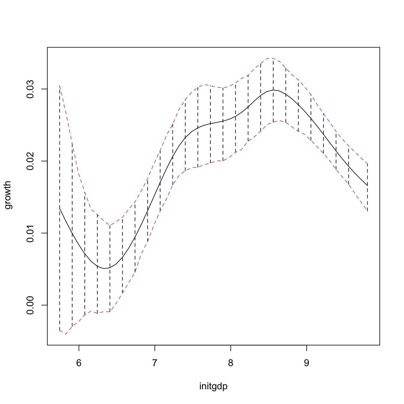

# These bootstrap standard errors are different from the asymptotic ones,
# and also from the previous bootstrap errors (different confidence
# interval method)
head(npplot_qua$r1$merr)
##              [,1]        [,2]
## [1,] -0.016923716 0.017015321
## [2,] -0.015649920 0.015060896
## [3,] -0.012913035 0.012441999
## [4,] -0.010752339 0.009864879
## [5,] -0.008496998 0.008547620
## [6,] -0.006912847 0.007220871

There is no predict() method featuring bootstrap confidence intervals, it has to be coded manually! This is the purpose of the next function, np_pred_CI(), which implements the naive bootstrap procedure described above to compute bootstrap confidence intervals for \(m(\mathbf{x}).\)

# Function to predict and compute bootstrap confidence intervals for m(x). Takes
# as main arguments a np::npreg object (npfit) and the values of the predictors
# where to carry out prediction (exdat). Requires that exdat is a data.frame of
# the same type than the one used for the predictors (e.g., there will be an
# error if one variable appears as a factor for computing npfit and then is
# passed as a numeric in exdat)
np_pred_CI <- function(npfit, exdat, B = 200, conf = 0.95,
                       type_CI = c("standard", "quantiles")[1]) {

  # Extract predictors
  xdat <- npfit$eval

  # Extract response, using a trick from np::npplot.rbandwidth
  tt <- terms(npfit$bws)
  tmf <- npfit$bws$call[c(1, match(c("formula", "data"),
                                   names(npfit$bws$call)))]
  tmf[[1]] <- as.name("model.frame")
  tmf[["formula"]] <- tt
  tmf <- eval(tmf, envir = environment(tt))
  ydat <- model.response(tmf)

  # Predictions
  m_hat <- np::npreg(txdat = xdat, tydat = ydat, exdat = exdat,
                     bws = npfit$bws)$mean

  # Function for performing Step 3
  boot_function <- function(data, indices) {

    np::npreg(txdat = xdat[indices,], tydat = ydat[indices],
              exdat = exdat, bws = npfit$bws)$mean

  }

  # Carry out Step 3
  m_hat_star <- boot::boot(data = data.frame(xdat), statistic = boot_function,
                           R = B)$t

  # Confidence intervals
  alpha <- 1 - conf
  if (type_CI == "standard") {

    z <- qnorm(p = 1 - alpha / 2)
    se <- apply(m_hat_star, 2, sd)
    lwr <- m_hat - z * se
    upr <- m_hat + z * se

  } else if (type_CI == "quantiles") {

    q <- apply(m_hat_star, 2, quantile, probs = c(alpha / 2, 1 - alpha / 2))
    lwr <- q[1, ]
    upr <- q[2, ]

  } else {

    stop("Incorrect type_CI")

  }

  # Return evaluation points, estimates, and confidence intervals
  return(data.frame("exdat" = exdat, "m_hat" = m_hat, "lwr" = lwr, "upr" = upr))

}

# Obtain predictions and confidence intervals along a fine grid, using the
# same seed employed by np::npplot for proper comparison
set.seed(42)
ci1 <- np_pred_CI(npfit = fit1, B = B, exdat = seq(5, 10, by = 0.01),
                  type_CI = "quantiles")

# Reconstruction of np::npplot's figure -- the curves coincide perfectly
plot(fit1, plot.errors.method = "bootstrap", plot.errors.type = "quantiles",
     plot.errors.boot.num = B, plot.errors.style = "bar", lwd = 3)
lines(npplot_qua$r1$eval[, 1], npplot_qua$r1$mean + npplot_qua$r1$merr[, 1],
      col = 2, lwd = 3)
lines(npplot_qua$r1$eval[, 1], npplot_qua$r1$mean + npplot_qua$r1$merr[, 2],
      col = 2, lwd = 3)
lines(ci1$exdat, ci1$m_hat, col = 3)
lines(ci1$exdat, ci1$lwr, col = 4)
lines(ci1$exdat, ci1$upr, col = 4)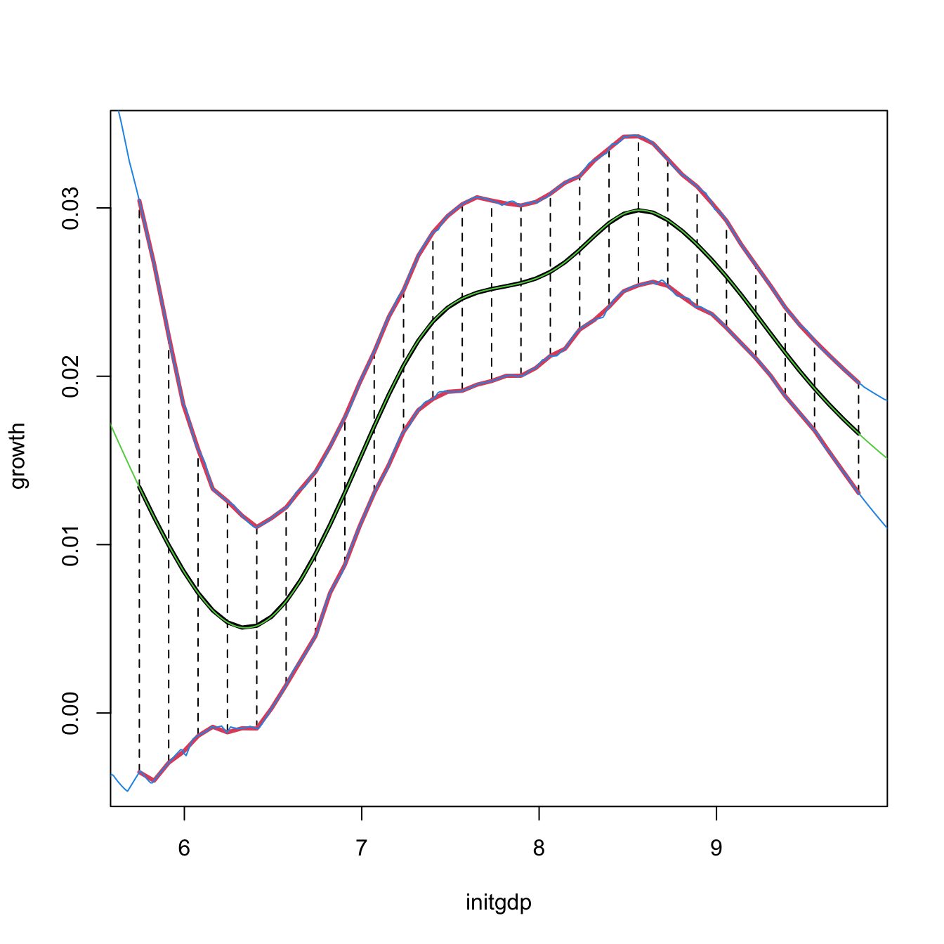

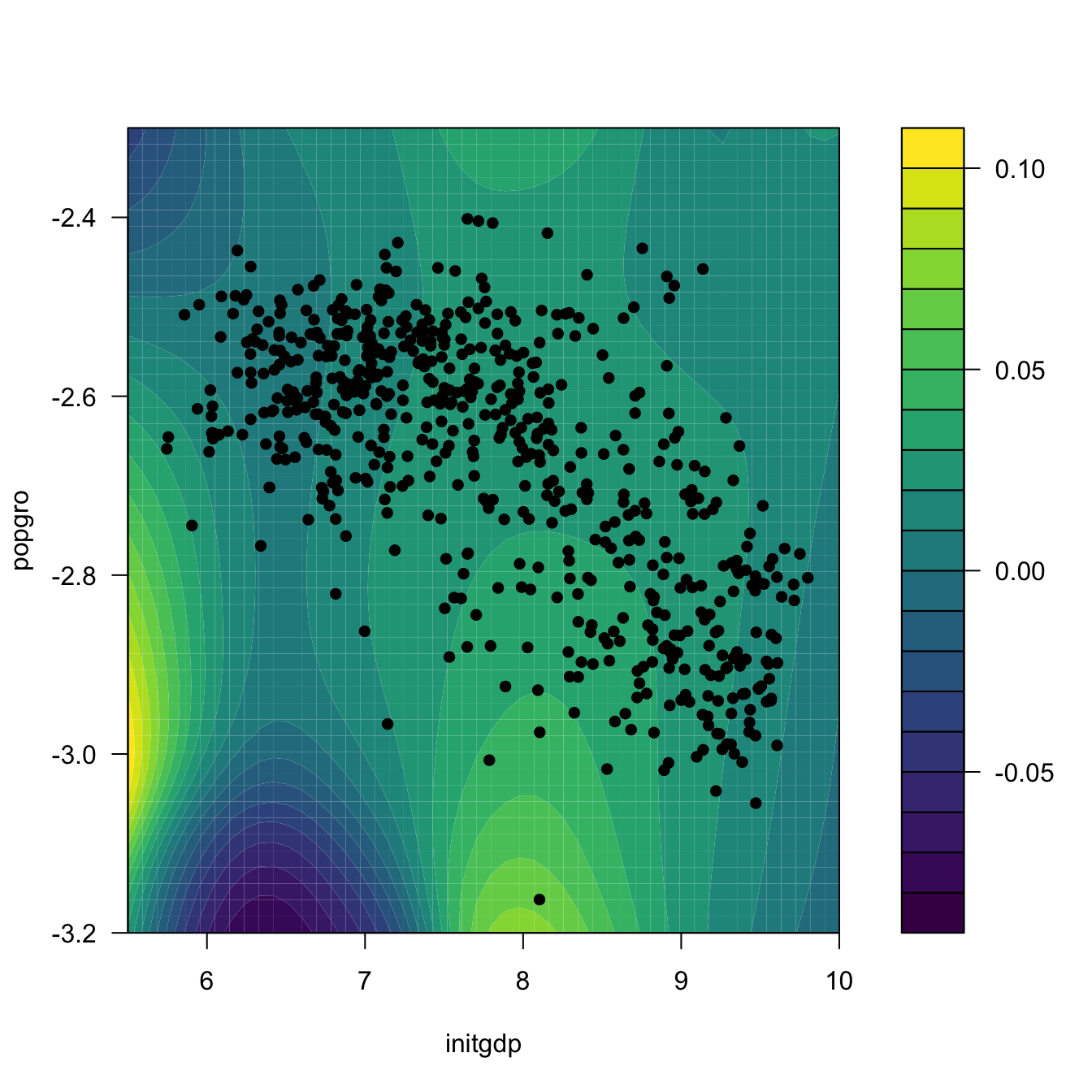
# But np_pred_CI is also valid for regression models with several predictors!
# An example with bivariate local linear regression with CV bandwidth
bw2 <- np::npregbw(formula = growth ~ initgdp + popgro, data = oecdpanel,
                   regtype = "ll")
fit2 <- np::npreg(bw2)

# Predictions and confidence intervals along a bivariate grid
L <- 50
x_initgdp <- seq(5.5, 10, l = L)
x_popgro <- seq(-3.2, -2.3, l = L)
exdat <- expand.grid(x_initgdp, x_popgro)
ci2 <- np_pred_CI(npfit = fit2, exdat = exdat)

# Regression surface. Observe the extrapolatory artifacts for
# low-density regions
m_hat <- matrix(ci2$m_hat, nrow = L, ncol = L)
filled.contour(x_initgdp, x_popgro, m_hat, nlevels = 20,
               color.palette = viridis::viridis,
               xlab = "initgdp", ylab = "popgro",
               plot.axes = {
                 axis(1); axis(2);
                 points(popgro ~ initgdp, data = oecdpanel, pch = 16)
                 })

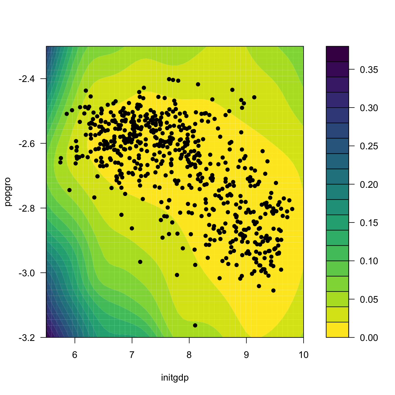
# Length of the 95%-confidence intervals for the regression. Observe how
# they grow for low-density regions
ci_dif <- matrix(ci2$upr - ci2$lwr, nrow = L, ncol = L)
filled.contour(x_initgdp, x_popgro, ci_dif, nlevels = 20,
               color.palette = function(n) viridis::viridis(n, direction = -1),
               xlab = "initgdp", ylab = "popgro",
               plot.axes = {
                 axis(1); axis(2);
                 points(popgro ~ initgdp, data = oecdpanel, pch = 16)
                 })

Exercise 5.8 Split the data(Auto, package = "ISLR") dataset by taking set.seed(12345); ind_train <- sample(nrow(Auto), size = nrow(Auto) - 12) as the index for the training dataset and use the remaining observations for the validation dataset. Then, for the regression problem described in Exercise 5.5:

1. Fit the local constant and linear estimators with CV bandwidths by taking the nature of the variables into account. Hint: remember using ordered and factor if necessary.
2. Interpret the nonparametric fits via marginal effects (for the quantile \(0.5\)) and bootstrap confidence intervals.
3. Obtain the mean squared prediction error on the validation dataset for the two fits. Which estimate gives the lowest error?
4. Compare the errors with the ones made by a linear estimation. Which approach gives lowest errors?

Exercise 5.9 The data(ChickWeight) dataset in R contains \(578\) observations of the weight, Time, and Diet of chicks. Consider the regression weight ~ Time + Diet.

1. Fit the local linear estimator with CV bandwidths by taking the nature of the variables into account.
2. Plot the marginal effects of Time for the four possible types of Diet. Overlay the four samples and use different colors. Explain your interpretations.
3. Obtain the bootstrap \(90\%\)-confidence intervals of the expected weight of a chick on the 20th day, for each of the four types of diets (take \(B=500\)). With a \(90\%\) confidence, state which diet dominates in terms of weight the other diets, and which are comparable.
4. Produce a plot that shows the extrapolation of the expected weight, for each of the four diets, from the 20th to the 30th day. Add bootstrap \(90\%\)-confidence bands. Explain your interpretations.

Exercise 5.10 Investigate the accuracy of the confidence intervals implemented in np::npplot for a fixed bandwidth \(h\). To do so:

1. Simulate \(M=500\) samples of size \(n=100\) from the regression model \(Y=m(X)+\varepsilon,\) where \(m(x) = 0.25x^2 - 0.75x + 3,\) \(X\sim\mathcal{N}(0,1.5^2),\) and \(\varepsilon\sim\mathcal{N}(0,0.75^2).\)
2. Compute the \(95\%\)-confidence intervals for \(m(x)\) along x <- seq(-5, 5, by = 0.1), for each of the \(M\) samples. Do it for the normal approximation and quantile-based confidence intervals.
3. Check if \(m(x)\) belongs to each of the confidence intervals, for each \(x.\)
4. Approximate the actual coverage of the confidence intervals, for each \(x.\)

Once you have a working solution, increase \(n\) to \(n=200,500,\) consider other regression models \(m,\) and summarize your conclusions. Explore the effect of different bandwidth values. Use \(B=500.\)

Naive bootstrap, although conceptually simple, does not capture the uncertainty of \(\hat{m}(\mathbf{x};q,\mathbf{h})\) in all situations, and may severely underestimate the variability of \(\hat{m}(\mathbf{x};q,\mathbf{h}).\) A more sophisticated bootstrap procedure is the so-called wild bootstrap (Wu 1986; Liu 1988; Hardle and Marron 1991), as it is a resampling strategy particularly well-suited for regression problems with heteroscedasticity. The wild bootstrap approach replaces Step 2 in the previous bootstrap resampling with:

1. Simulate \(V_1^{*b},\ldots,V_n^{*b}\) to be iid copies of \(V\) such that \(\mathbb{E}[V]=0\) and \(\mathbb{V}\mathrm{ar}[V]=1.\)¹⁸⁸
2. Compute the perturbed residuals \(\varepsilon_i^{*b}:=\hat\varepsilon_iV_i^{*b},\) where \(\hat\varepsilon_i:=Y_i-\hat{m}(\mathbf{X}_i;q,\mathbf{h}),\) \(i=1,\ldots,n.\)
3. Obtain the bootstrap sample \((\mathbf{X}_1,Y_1^{*b}),\ldots,(\mathbf{X}_n,Y_n^{*b}),\) where \(Y_i^{*b}:=\hat{m}(\mathbf{X}_i;q,\mathbf{h})+\varepsilon_i^{*b},\) \(i=1,\ldots,n.\)
4. Compute \(\hat{m}^{*b}(\mathbf{x};q,\mathbf{h})=\sum_{i=1}^n W_i^{q}(\mathbf{x})Y_i^{*b}\) from \((\mathbf{X}_1,Y_1^{*b}),\ldots,(\mathbf{X}_n,Y_n^{*b}).\)

Unfortunately, np does not seem to implement the wild bootstrap. The next exercise points to its implementation.

Exercise 5.11 Adapt the np_pred_CI function to include the argument type_boot, which can take either the value "naive" or "wild". If type_boot = "wild", then the function must compute wild bootstrap confidence intervals, implementing from scratch Steps i–iv of the wild bootstrap resampling. Validate the correct behavior of the wild bootstrap confidence intervals in the simulation study described in Exercise 5.10, but considering a single sample size \(n\) and regression model \(m.\)

5.4 Local likelihood

We next explore an extension of the local polynomial estimator that imitates the expansion that generalized linear models made of linear models, allowing the former to consider non-continuous responses. This extension is aimed to estimate the regression function by relying on the likelihood, rather than the least squares. The main idea behind local likelihood is, therefore, to locally fit parametric models by maximum likelihood.

We begin by seeing that local likelihood based on the linear model is equivalent to local polynomial modeling. Theorem B.1 shows that, under the assumptions given in Section B.1.2, the maximum likelihood estimate of \(\boldsymbol{\beta}\) in the linear model

\[\begin{align} Y \mid (X_1,\ldots,X_p)\sim\mathcal{N}(\beta_0+\beta_1X_1+\cdots+\beta_pX_p,\sigma^2)\tag{5.15} \end{align}\]

is equivalent to the least squares estimate, \(\hat{\boldsymbol{\beta}}=(\mathbf{X}^\top\mathbf{X})^{-1}\mathbf{X}^\top\mathbf{Y}.\) The reason for this is the form of the conditional (on \(X_1,\ldots,X_p\)) log-likelihood:

\[\begin{align*} \ell(\boldsymbol{\beta})=&-\frac{n}{2}\log(2\pi\sigma^2)\nonumber\\ &-\frac{1}{2\sigma^2}\sum_{i=1}^n(Y_i-\beta_0-\beta_1X_{i1}-\cdots-\beta_pX_{ip})^2. \end{align*}\]

If there is a single predictor \(X,\) the situation on which we focus on, a polynomial fitting of order \(p\) of the conditional mean can be achieved by the well-known trick of identifying the \(j\)-th predictor \(X_j\) in (5.15) by \(X^j.\)¹⁸⁹ This results in

\[\begin{align} Y \mid X\sim\mathcal{N}(\beta_0+\beta_1X+\cdots+\beta_pX^p,\sigma^2).\tag{5.16} \end{align}\]

Therefore, we can define the weighted log-likelihood of the linear model (5.16) about \(x\) as

\[\begin{align} \ell_{x,h}(\boldsymbol{\beta}):=& -\frac{n}{2}\log(2\pi\sigma^2)\tag{5.17}\\ &-\frac{1}{2\sigma^2}\sum_{i=1}^n(Y_i-\beta_0-\beta_1(X_i-x)-\cdots-\beta_p(X_i-x)^p)^2K_h(x-X_i).\nonumber \end{align}\]

Maximizing with respect to \(\boldsymbol{\beta}\) the local log-likelihood (5.17) provides \(\hat\beta_0=\hat{m}(x;p,h),\) which is precisely the local polynomial estimator, as it was obtained in (4.10), but now obtained from a likelihood-based perspective. The key point is to realize that the very same idea can be applied to the family of generalized linear models, for which linear regression (in this case manifested as a polynomial regression) is just a particular case.

Figure 5.1: Construction of the local likelihood estimator. The animation shows how local likelihood fits in a neighborhood of \(x\) are combined to provide an estimate of the regression function for binary response, which depends on the polynomial degree, bandwidth, and kernel (gray density at the bottom). The data points are shaded according to their weights for the local fit at \(x.\) Application available here.

We illustrate the local likelihood principle for the logistic regression (see Section B.2 for a quick review). In this case, the sample is \((X_1,Y_1),\ldots,(X_n,Y_n)\) with

\[\begin{align*} Y_i \mid X_i\sim \mathrm{Ber}(\mathrm{logistic}(\eta(X_i))),\quad i=1,\ldots,n, \end{align*}\]

with the polynomial term¹⁹⁰

\[\begin{align*} \eta(x):=\beta_0+\beta_1x+\cdots+\beta_px^p. \end{align*}\]

The log-likelihood of \(\boldsymbol{\beta}\) is

\[\begin{align*} \ell(\boldsymbol{\beta})=&\,\sum_{i=1}^n\left\{Y_i\log(\mathrm{logistic}(\eta(X_i)))+(1-Y_i)\log(1-\mathrm{logistic}(\eta(X_i)))\right\}\nonumber\\ =&\,\sum_{i=1}^n\ell(Y_i,\eta(X_i)), \end{align*}\]

where we consider the log-likelihood addend \(\ell(y,\eta):=y\eta-\log(1+e^\eta).\) For the sake of clarity in the next developments, we make explicit the dependence on \(\eta(x)\) of this addend; conversely, we make its dependence on \(\boldsymbol{\beta}\) implicit.

The local log-likelihood of \(\boldsymbol{\beta}\) about \(x\) is then defined as

\[\begin{align} \ell_{x,h}(\boldsymbol{\beta}):=\sum_{i=1}^n\ell(Y_i,\eta(X_i-x))K_h(x-X_i).\tag{5.18} \end{align}\]

Maximizing¹⁹¹ the local log-likelihood (5.18) with respect to \(\boldsymbol{\beta}\) provides

\[\begin{align*} \hat{\boldsymbol{\beta}}_{h}=\arg\max_{\boldsymbol{\beta}\in\mathbb{R}^{p+1}}\ell_{x,h}(\boldsymbol{\beta}). \end{align*}\]

The local likelihood estimate of \(\eta(x)\) is the intercept of this fit,

\[\begin{align*} \hat\eta(x):=\hat\beta_{h,0}. \end{align*}\]

Note that the dependence of \(\hat\beta_{h,0}\) on \(x\) is omitted. From \(\hat\eta(x),\) we can obtain the local logistic regression evaluated at \(x\) as¹⁹²

\[\begin{align} \hat{m}_{\ell}(x;p,h):=g^{-1}\left(\hat\eta(x)\right)=\mathrm{logistic}(\hat\beta_{h,0}).\tag{5.19} \end{align}\]

Each evaluation of \(\hat{m}_{\ell}(x;p,h)\) in a different \(x\) requires, thus, a weighted fit of the underlying local logistic model.

The code below shows three different ways of implementing in R the local logistic regression (with \(p=1\)).

# Simulate some data
n <- 200
logistic <- function(x) 1 / (1 + exp(-x))
p <- function(x) logistic(1 - 3 * sin(x))
set.seed(123456)
X <- sort(runif(n = n, -3, 3))
Y <- rbinom(n = n, size = 1, prob = p(X))

# Set bandwidth and evaluation grid
h <- 0.25
x <- seq(-3, 3, l = 501)

# Approach 1: optimize the weighted log-likelihood through the workhorse
# function underneath glm, glm.fit
suppressWarnings(
  fit_glm <- sapply(x, function(x) {
    K <- dnorm(x = x, mean = X, sd = h)
    glm.fit(x = cbind(1, X - x), y = Y, weights = K,
            family = binomial())$coefficients[1]
  })
)

# Approach 2: optimize directly the weighted log-likelihood
suppressWarnings(
  fit_nlm <- sapply(x, function(x) {
    K <- dnorm(x = x, mean = X, sd = h)
    nlm(f = function(beta) {
      -sum(K * (Y * (beta[1] + beta[2] * (X - x)) -
                  log(1 + exp(beta[1] + beta[2] * (X - x)))))
      }, p = c(0, 0))$estimate[1]
  })
)

# Approach 3: employ locfit::locfit
# CAREFUL: locfit::locfit uses a different internal parametrization for h!
# As it can be seen, the bandwidths in approaches 1-2 and approach 3 do NOT
# give the same results! With h = 0.75 in locfit::locfit the fit is close
# to the previous ones (done for h = 0.25), but not exactly the same...
fit_locfit <- locfit::locfit(Y ~ locfit::lp(X, deg = 1, h = 0.75),
                             family = "binomial", kern = "gauss")

# Compare fits
plot(x, p(x), ylim = c(0, 1.5), type = "l", lwd = 2)
lines(x, logistic(fit_glm), col = 2, lwd = 2)
lines(x, logistic(fit_nlm), col = 3, lty = 2)
lines(x, predict(fit_locfit, newdata = x), col = 4)
legend("topright", legend = c("p(x)", "glm", "nlm", "locfit"),
       lwd = 2, col = c(1, 2, 3, 4), lty = c(1, 1, 2, 1))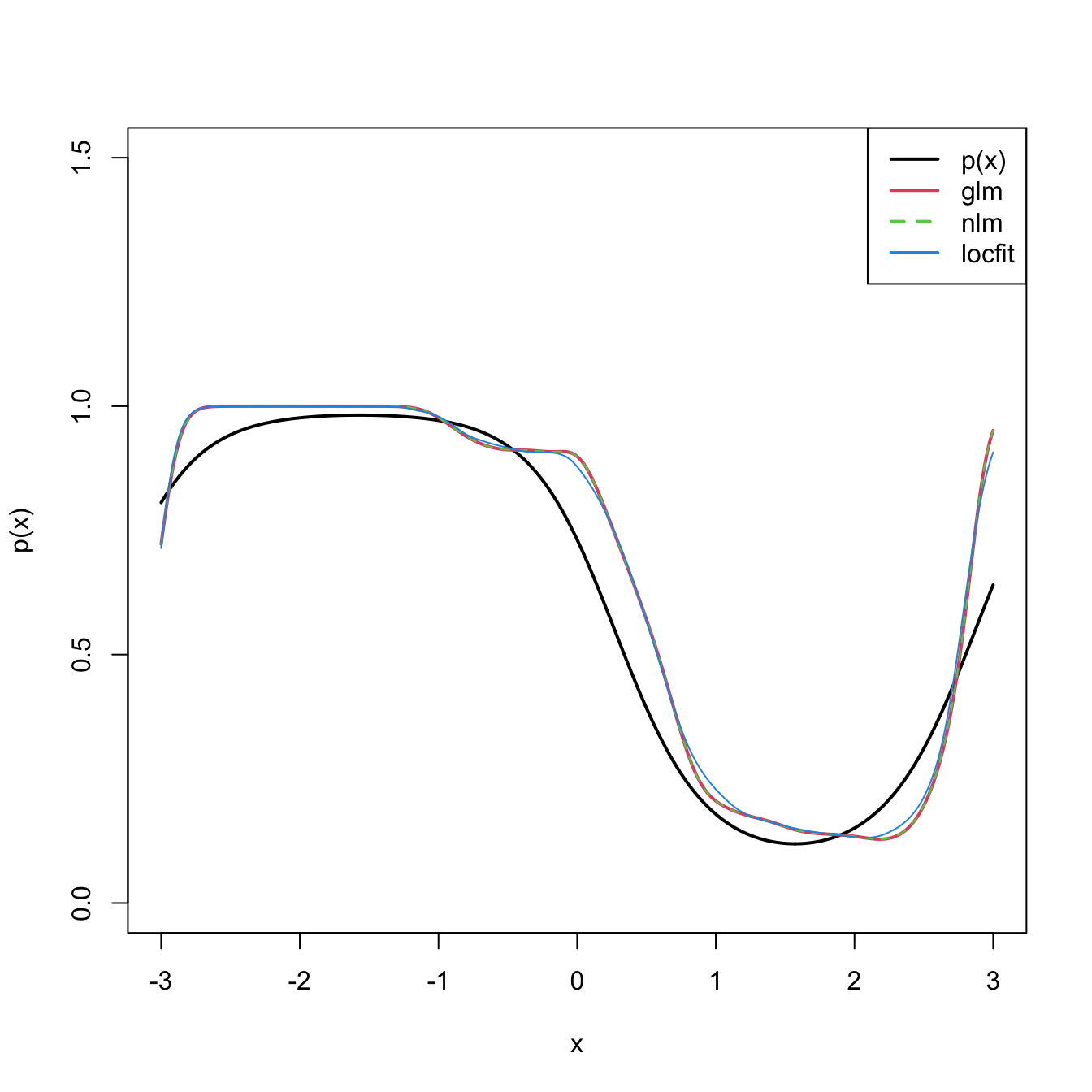

Bandwidth selection can be done by means of likelihood cross-validation. The objective is to maximize the local log-likelihood fit at \((X_i,Y_i)\) but removing the influence by the datum itself. That is,

\[\begin{align} \hat{h}_{\mathrm{LCV}}&=\arg\max_{h>0}\mathrm{LCV}(h),\nonumber\\ \mathrm{LCV}(h)&=\sum_{i=1}^n\ell(Y_i,\hat\eta_{-i}(X_i)),\tag{5.20} \end{align}\]

where \(\hat\eta_{-i}(X_i)\) represents the local fit at \(X_i\) without the \(i\)-th datum \((X_i,Y_i).\)¹⁹³ Unfortunately, the nonlinearity of (5.19) forbids a simplifying result as the one in Proposition 4.1. Thus, in principle, it is required to fit \(n\) local likelihoods for sample size \(n-1\) to obtain a single evaluation of (5.20).¹⁹⁴

We conclude by illustrating how to compute the LCV function and optimize it. Keep in mind that much more efficient implementations are possible!

# Exact LCV - recall that we *maximize* the LCV!
h <- seq(0.1, 2, by = 0.1)
suppressWarnings(
  LCV <- sapply(h, function(h) {
  sum(sapply(1:n, function(i) {
    K <- dnorm(x = X[i], mean = X[-i], sd = h)
    nlm(f = function(beta) {
      -sum(K * (Y[-i] * (beta[1] + beta[2] * (X[-i] - X[i])) -
                  log(1 + exp(beta[1] + beta[2] * (X[-i] - X[i])))))
      }, p = c(0, 0))$minimum
    }))
  })
)
plot(h, LCV, type = "o")
abline(v = h[which.max(LCV)], col = 2)

Exercise 5.12 (Adapted from Example 4.6 in Wasserman (2006)) The dataset at http://www.stat.cmu.edu/~larry/all-of-nonpar/=data/bpd.dat (alternative link) contains information about the presence of bronchopulmonary dysplasia (binary response) and the birth weight in grams (predictor) of \(223\) newborns.

1. Use the three approaches described above to compute the local logistic regression (first degree) and plot their outputs for a bandwidth that is somewhat adequate.
2. Using \(\hat{h}_{\mathrm{LCV}},\) explore and comment on the resulting estimates, providing insights into the data.
3. From the obtained fit, derive several simple medical diagnostic rules for the probability of the presence of bronchopulmonary dysplasia from the birth weight.

Exercise 5.13 The challenger.txt dataset contains information regarding the state of the solid rocket boosters after launch for \(23\) shuttle flights prior to the Challenger launch. Each row has, among others, the variables fail.field (indicator of whether there was an incident with the O-rings), nfail.field (number of incidents with the O-rings), and temp (temperature in the day of launch, measured in Celsius degrees). See Section 5.1 in García-Portugués (2025) for further context on the Challenger case study.

1. Fit a local logistic regression (first degree) for fails.field ~ temp, for three choices of bandwidths: one that oversmooths, another that is somewhat adequate, and another that undersmooths. Do the effects of temp on fails.field seem to be significant?
2. Obtain \(\hat{h}_{\mathrm{LCV}}\) and plot the LCV function with a reasonable accuracy.
3. Using \(\hat{h}_{\mathrm{LCV}},\) predict the probability of an incident at temperatures \(-0.6\) (launch temperature of the Challenger) and \(11.67\) (vice president of engineers’ recommended launch threshold).
4. What are the local odds at \(-0.6,\) \(11.67,\) and \(20\)? Show the local logistic models about these points, in spirit of Figure 5.1, and interpret the results.

Exercise 5.14 Implement your own version of the local likelihood estimator (first degree) for the Poisson regression model. To do so:

1. Derive the local log-likelihood about \(x\) for the Poisson regression (which is analogous to (5.18)). You can check Section 5.2.2 in García-Portugués (2025) for information on the Poisson regression.
2. Code from scratch an R function, loc_pois, that maximizes the previous local likelihood for a vector of evaluation points. loc_pois must take as input the samples X and Y, the vector of evaluation points x, the bandwidth h, and the kernel K.
3. Implement a cv_loc_pois function that obtains the likelihood cross-validated bandwidth for the local Poisson regression.
4. Validate the correct behavior of loc_pois and cv_loc_pois by sampling a sample of \(n=200\) from \(Y \mid X=x \sim \mathrm{Poisson}(\lambda(x)),\) where \(\lambda(x)=e^{\sin(x)}\) and \(X\) is distributed according to a nor1mix::MW.nm7.
5. Compare your results with the locfit::locfit function using family = "poisson" (you should not expect an exact fit due to the different parametrization of h used in the locfit::locfit function, as warned in the previous explanatory code chunk).

References

Aitchison, J., and C. G. G. Aitken. 1976. “Multivariate Binary Discrimination by the Kernel Method.” Biometrika 63 (3): 413–20. https://doi.org/10.1093/biomet/63.3.413.

García-Portugués, E. 2025. Notes for Predictive Modeling. https://egarpor.github.io/PM-UC3M/.

Hardle, W., and J. S. Marron. 1991. “Bootstrap Simultaneous Error Bars for Nonparametric Regression.” The Annals of Statistics 19 (2): 778–96. https://doi.org/10.1214/aos/1176348120.

Hayfield, T., and J. S. Racine. 2008. “Nonparametric Econometrics: The np Package.” Journal of Statistical Software 27 (5): 1–32. https://doi.org/10.18637/jss.v027.i05.

Li, Q., and J. S. Racine. 2007. Nonparametric Econometrics. Princeton: Princeton University Press. https://press.princeton.edu/books/hardcover/9780691121611/nonparametric-econometrics.

Liu, R. Y. 1988. “Bootstrap Procedures Under Some Non-i.i.d. Models.” The Annals of Statistics 16 (4): 1696–1708. https://doi.org/10.1214/aos/1176351062.

Loader, C. 1999. Local Regression and Likelihood. Statistics and Computing. New York: Springer. https://doi.org/10.2307/1270956.

Molnar, C. 2024. Interpretable Machine Learning. https://christophm.github.io/interpretable-ml-book/.

———. 2006. All of Nonparametric Statistics. Springer Texts in Statistics. New York: Springer. https://doi.org/10.1007/0-387-30623-4.

Wu, C. F. J. 1986. “Jackknife, Bootstrap and Other Resampling Methods in Regression Analysis.” The Annals of Statistics 14 (4): 1261–95. https://doi.org/10.1214/aos/1176350142.

---

166. Local polynomial estimators also “work” with discrete responses, with a varying degree of adequacy. For example, if \(Y\) is binary, then \(\hat m_h(x;0,h)\in[0,1],\) for any \(x\in\mathbb{R}\) and \(h>0,\) since \(\hat m_h(x;0,h)\) is an \(x\)-weighted mean (or a convex linear combination) of \(Y_1,\ldots,Y_n\in[0,1].\) Then, the regression function \(m:\mathbb{R}\longrightarrow[0,1]\) is always properly estimated. However, a local linear estimator may yield improper estimators of \(m,\) since \(\hat m_h(x;1,h)\) is an \(x\)-weighted linear combination of \(Y_1,\ldots,Y_n\in[0,1]\) and consequently \(\hat m_h(x;1,h)\) may “spike” outside \([0,1].\)↩︎

167. Here \(q\) denotes the order of the polynomial fit, since \(p\) stands for the number of predictors.↩︎

168. In particular, the consideration of Taylor expansions of \(m:\mathbb{R}^p\longrightarrow\mathbb{R}\) for more than two orders that involve the vector of partial derivatives \(\mathrm{D}^{\otimes s}m(\mathbf{x}),\) formed by \(\frac{\partial^s m(\mathbf{x})}{\partial x_1^{s_1}\cdots \partial x_p^{s_p}},\) where \(s=s_1+\cdots+s_p;\) see Section 3.1.↩︎

169. Observe that in the second equality we assume that \(Y \mid \mathbf{X}=\mathbf{x}\) is continuous.↩︎

170. Assuming that \((\mathbf{X},Y)\) is continuous to motivate the construction of the estimator.↩︎

171. The fact that the kde for \((\mathbf{X},Y)\) has a product kernel between the variables \(\mathbf{X}\) and \(Y\) is not fundamental for constructing the Nadaraya–Watson estimator, but it simplifies the computation of the integral of the denominator of (5.2). The fact that the bandwidth matrices for estimating the \(\mathbf{X}\)-part of \(f\) and the marginal \(f_\mathbf{X}\) are equal, is fundamental to ensure an estimator for \(m\) that is a weighted average (with weights adding one) of the responses \(Y_1,\ldots,Y_n.\)↩︎

172. Which increases at the order \(O(p^2).\)↩︎

173. Observe that \((X_i-x)^j\) are replaced with \((X_{ij}-x_j),\) since we only consider a linear fit and now the predictors have \(p\) components.↩︎

174. Observe that, in an abuse of notation, we denote both the random vector \((X_1,\ldots,X_p)\) and the design matrix by \(\mathbf{X}.\) However, the specific meaning of \(\mathbf{X}\) should be clear from the context.↩︎

175. Recall that now the entries of \(\hat{\boldsymbol{\beta}}_\mathbf{h}\) are estimating \(\boldsymbol{\beta}=\begin{pmatrix}m(\mathbf{x})\\\mathrm{D} m(\mathbf{x})\end{pmatrix}.\) So, \(\hat{\boldsymbol{\beta}}_\mathbf{h}\) gives also an estimate of the gradient \(\mathrm{D} m\) evaluated at \(\mathbf{x}.\)↩︎

176. See Section 9.1 of Molnar (2024) and references therein.↩︎

177. See Section 8.1 of Molnar (2024) and references therein.↩︎

178. \(\hat{Y}_i:=\hat{m}(\mathbf{X}_i;q,\mathbf{h}),\) \(i=1,\ldots,n;\) see Section 5.3.↩︎

179. Because it is not guaranteed that \(\bar{Y}=\bar{\hat{Y}},\) what it is required to turn \(R^2\) into that squared correlation coefficient.↩︎

180. Although in practice it is not required for the kernel to integrate to one for performing regression, as the constants of the kernels cancel out in the quotients in \(\hat{m}(\cdot;q,\mathbf{h}).\)↩︎

181. Recall \(K_h(x-X_i).\)↩︎

182. Notice that this kernel does not integrate to one! To normalize it we should take the specific support of \(X_d\) into account, which, e.g., could be \(\{0, 1, 2, 3\}\) or \(\mathbb{N}.\) This is slightly cumbersome, so we avoid it because there is no difference between normalized and unnormalized kernels for regression: the kernel normalizing constants cancel out in the computation of the weights (5.12).↩︎

183. Importantly, note that this kernel is assuming that the levels are equally-separated! Care is needed in applications when dealing with unequally-separated ordinal variables and using ordered with the default levels specification.↩︎

184. Precisely, the ones associated with the asymptotic normality of \(\hat{m}(\mathbf{x};q,\mathbf{h})\) and that are collected in Theorem 4.2 for the case of a single continuous predictor.↩︎

185. As usable asymptotic approximations are hampered by two factors: (i) the slow convergence speed towards the asymptotic distribution (recall the effective sample size in Theorem 4.2); and (ii) the need to estimate the unknown terms in the asymptotic bias and variance, which leads to an endless cycle (similar to that in Section 2.4.1).↩︎

186. This is the same as randomly accessing \(n\) times the rows of the matrix \(\begin{pmatrix} X_{11} & \ldots & X_{1p} & Y_1 \\ \vdots & \ddots & \vdots & \vdots \\ X_{n1} & \ldots & X_{np} & Y_n \end{pmatrix}_{n\times(p+1)}.\)↩︎

187. Although this might be confusing, since Hayfield and Racine (2008) states that “Specifying the type of bootstrapping as ‘inid’ admits general heteroscedasticity of unknown form via the wild bootstrap (Liu 1988), though it does not allow for dependence.” but, as of version 0.60-10, the naive bootstrap is run when plot.errors.boot.method = "inid" (see code).↩︎

188. For example, the golden section binary variable defined by \(\mathbb{P}[V=1-\phi]=p\) and \(\mathbb{P}[V=\phi]=1-p,\) with \(\phi=(1+\sqrt{5})/2\) and \(p=(\phi+2)/5.\)↩︎

189. Observe that, for the sake of easier presentation, we return to the notation and setting employed in Chapter 4, in which only one predictor \(X\) was available for explaining \(Y,\) and where \(p\) denoted the order of the polynomial fit employed.↩︎

190. If \(p=1,\) then we have the usual simple logistic model. Notice that we are just doing the “polynomial trick” done in linear regression, which consisted in expanding the number of predictors with the powers \(X^j,\) \(j=1,\ldots,p,\) of \(X\) to achieve more flexibility in the parametric fit.↩︎

191. There is no analytical solution for the optimization problem due to its nonlinearity, so a numerical approach is required.↩︎

192. An alternative and useful view is that, by maximizing (5.18), we are fitting the logistic model \(\hat{p}_x(t):=\mathrm{logistic}\big(\hat{\beta}_{h,0}+\hat{\beta}_{h,1}(t-x)+\cdots+\hat{\beta}_{h,p}(t-x)^p\big)\) that is centered about \(x.\) Then, we employ this model to predict \(Y\) for \(X=t=x,\) resulting \(\mathrm{logistic}\big(\hat{\beta}_{h,0}\big).\)↩︎

193. Observe that (5.20) is equivalent to (4.23) if the generalized linear model is a linear model.↩︎

194. The interested reader is referred to Sections 4.3.3 and 4.4.3 in Loader (1999) for an approximation of (5.20) that only requires a local likelihood fit for a single sample.↩︎