5 Generalized linear models
As we saw in Chapter 2, linear regression assumes that the response variable \(Y\) is such that
\[\begin{align*} Y \mid (X_1=x_1,\ldots,X_p=x_p)\sim \mathcal{N}(\beta_0+\beta_1x_1+\cdots+\beta_px_p,\sigma^2) \end{align*}\]
and hence
\[\begin{align*} \mathbb{E}[Y \mid X_1=x_1,\ldots,X_p=x_p]=\beta_0+\beta_1x_1+\cdots+\beta_px_p. \end{align*}\]
This, in particular, implies that \(Y\) is continuous. In this chapter we will see how generalized linear models can deal with other kinds of distributions for \(Y \mid (X_1=x_1,\ldots,X_p=x_p),\) particularly with discrete responses, by modeling the transformed conditional expectation. The simplest generalized linear model is logistic regression, which arises when \(Y\) is a binary response, that is, a variable encoding two categories with \(0\) and \(1.\) This model would be useful, for example, to predict \(Y\) given \(X\) from the sample \(\{(X_i,Y_i)\}_{i=1}^n\) in Figure 5.1.

Figure 5.1: Scatterplot of a sample \(\{(X_i,Y_i)\}_{i=1}^n\) sampled from a logistic regression.
5.1 Case study: The Challenger disaster
The Challenger disaster occurred on the 28th January of 1986, when the NASA Space Shuttle orbiter Challenger broke apart and disintegrated at 73 seconds into its flight, leading to the deaths of its seven crew members. The accident had serious consequences for NASA’s credibility and resulted in an interruption of 32 months in the shuttle program. The Presidential Rogers Commission (formed by astronaut Neil A. Armstrong and Nobel laureate Richard P. Feynman,147 among others) was created in order to investigate the causes of the disaster.
Figure 5.2: Challenger launch and subsequent explosion, as broadcast live by NBC in 28/01/1986. Video also available here.
The Rogers Commission elaborated a report (Presidential Commission on the Space Shuttle Challenger Accident 1986) with all the findings. The commission determined that the disintegration began with the failure of an O-ring seal in the solid rocket booster due to the unusually cold temperature (\(-0.6\) degrees Celsius; \(30.92\) degrees Fahrenheit) during the launch. This failure produced a breach of burning gas through the solid rocket booster that compromised the whole shuttle structure, resulting in its disintegration due to the extreme aerodynamic forces.
The problem with O-rings was something known. The night before the launch, there was a three-hour teleconference between rocket engineers at Thiokol, the manufacturer company of the solid rocket boosters, and NASA. In the teleconference, the effect on the O-rings performance of the low temperature forecasted for the launch was discussed, and eventually a launch decision was reached.148 Figure 5.3a influenced the data analysis conclusion that sustained the launch decision:
“Temperature data [is] not conclusive on predicting primary O-ring blowby.”
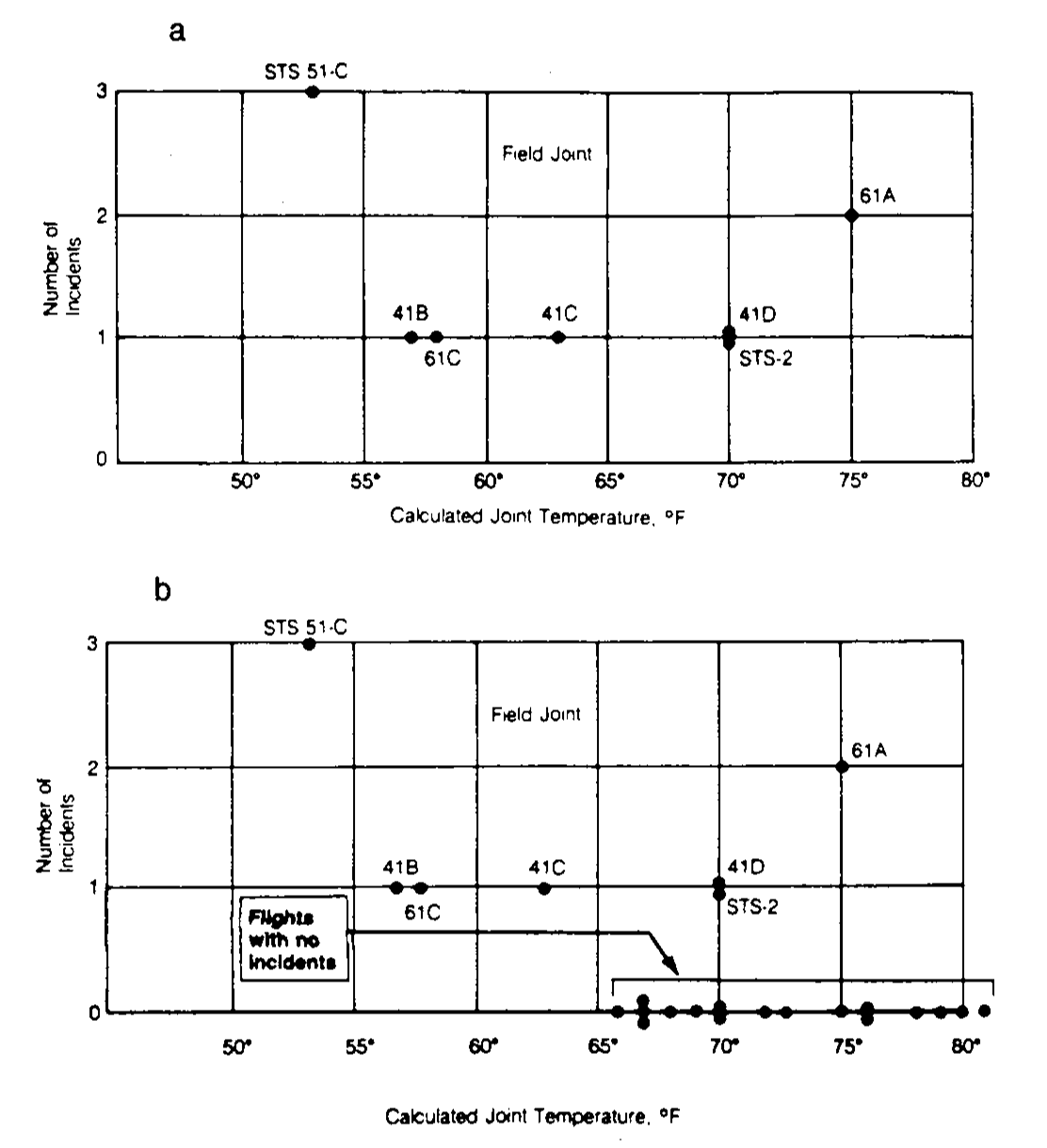
Figure 5.3: Number of incidents in the O-rings (filed joints) versus temperatures. Panel a includes only flights with incidents. Panel b contains all flights (with and without incidents).
The Rogers Commission noted a major flaw in Figure 5.3a, the one presented by the solid rocket booster engineers at the teleconference: the flights with zero incidents were excluded from the plot by the engineers because it was felt that these flights did not contribute any information about the temperature effect (Figure 5.3b). The Rogers Commission therefore concluded:
“A careful analysis of the flight history of O-ring performance would have revealed the correlation of O-ring damage in low temperature”.
The purpose of this case study, inspired by Siddhartha et al. (1989), is to quantify what was the influence of the temperature on the probability of having at least one incident related to the O-rings. Specifically, we want to address the following questions:
- Q1. Is the temperature associated with O-ring incidents?
- Q2. In which way was the temperature affecting the probability of O-ring incidents?
- Q3. What was the predicted probability of an incident in an O-ring for the temperature of the launch day?
- Q4. What was the predicted maximum probability of an incident in an O-ring if the launch were postponed until the temperature was above \(11.67\) degrees Celsius, as the vice president of engineers of Thiokol recommended?
To try to answer these questions, we analyze the challenger dataset (download), partially collected in Table 5.1. The dataset contains information regarding the state of the solid rocket boosters after launch149 for \(23\) flights prior to the Challenger launch. Each row has, among others, the following variables:
-
fail.field,fail.nozzle: binary variables indicating whether there was an incident with the O-rings in the field joints or in the nozzles of the solid rocket boosters.1codifies an incident and0its absence. For the analysis, we focus on the O-rings of the field joint as those were the most determinant for the accident. -
nfail.field,nfail.nozzle: number of incidents with the O-rings in the field joints and in the nozzles. -
temp: temperature in the day of launch, measured in degrees Celsius. -
pres.field,pres.nozzle: leak-check pressure tests of the O-rings. These tests assured that the rings would seal the joint.
| flight | date | nfails.field | nfails.nozzle | fail.field | fail.nozzle | temp |
|---|---|---|---|---|---|---|
| 1 | 12/04/81 | 0 | 0 | 0 | 0 | 18.9 |
| 2 | 12/11/81 | 1 | 0 | 1 | 0 | 21.1 |
| 3 | 22/03/82 | 0 | 0 | 0 | 0 | 20.6 |
| 5 | 11/11/82 | 0 | 0 | 0 | 0 | 20.0 |
| 6 | 04/04/83 | 0 | 2 | 0 | 1 | 19.4 |
| 7 | 18/06/83 | 0 | 0 | 0 | 0 | 22.2 |
| 8 | 30/08/83 | 0 | 0 | 0 | 0 | 22.8 |
| 9 | 28/11/83 | 0 | 0 | 0 | 0 | 21.1 |
| 41-B | 03/02/84 | 1 | 1 | 1 | 1 | 13.9 |
| 41-C | 06/04/84 | 1 | 1 | 1 | 1 | 17.2 |
| 41-D | 30/08/84 | 1 | 1 | 1 | 1 | 21.1 |
| 41-G | 05/10/84 | 0 | 0 | 0 | 0 | 25.6 |
| 51-A | 08/11/84 | 0 | 0 | 0 | 0 | 19.4 |
| 51-C | 24/01/85 | 2 | 2 | 1 | 1 | 11.7 |
| 51-D | 12/04/85 | 0 | 2 | 0 | 1 | 19.4 |
| 51-B | 29/04/85 | 0 | 2 | 0 | 1 | 23.9 |
| 51-G | 17/06/85 | 0 | 2 | 0 | 1 | 21.1 |
| 51-F | 29/07/85 | 0 | 0 | 0 | 0 | 27.2 |
| 51-I | 27/08/85 | 0 | 0 | 0 | 0 | 24.4 |
| 51-J | 03/10/85 | 0 | 0 | 0 | 0 | 26.1 |
| 61-A | 30/10/85 | 2 | 0 | 1 | 0 | 23.9 |
| 61-B | 26/11/85 | 0 | 2 | 0 | 1 | 24.4 |
| 61-C | 12/01/86 | 1 | 2 | 1 | 1 | 14.4 |
Let’s begin the analysis by replicating Figures 5.3a and 5.3b, and by checking that linear regression is not the right tool for addressing Q1–Q4.
# Read data
challenger <- read.table(file = "challenger.txt", header = TRUE, sep = "\t")
# Figures 5.3a and 5.3b
car::scatterplot(nfails.field ~ temp, smooth = FALSE, boxplots = FALSE,
                 data = challenger, subset = nfails.field > 0)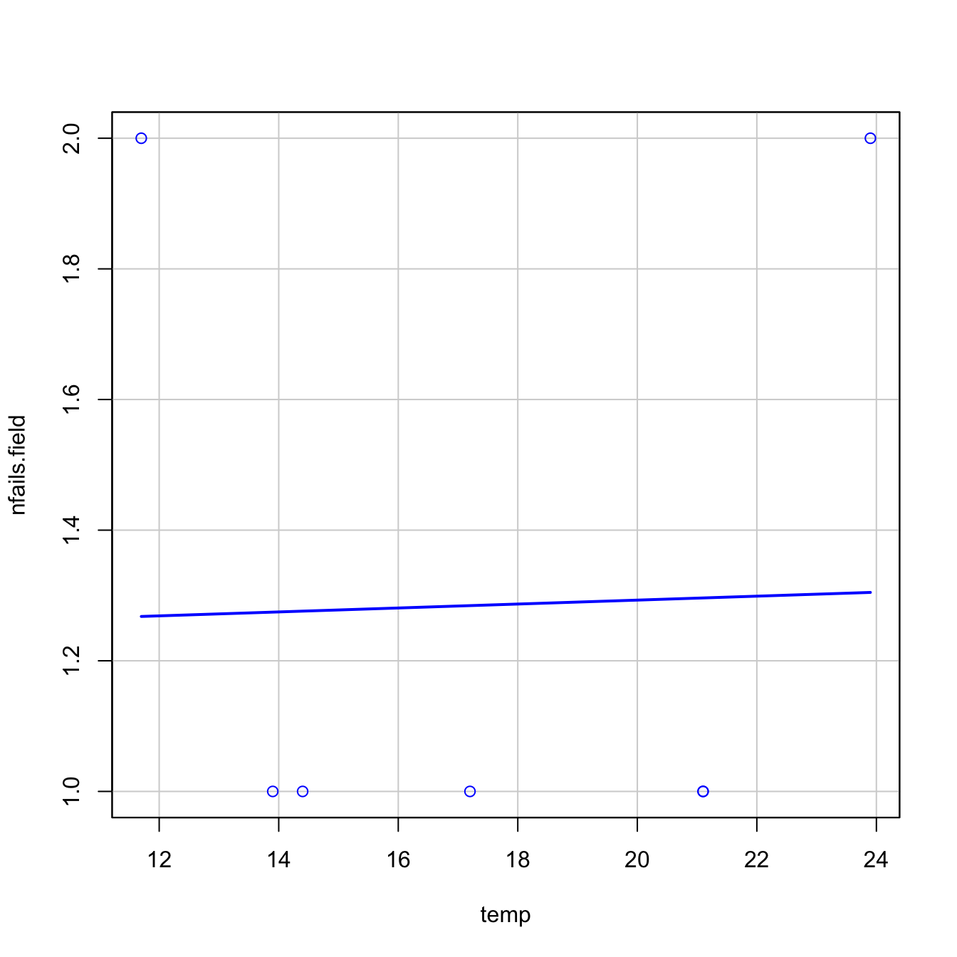
car::scatterplot(nfails.field ~ temp, smooth = FALSE, boxplots = FALSE,
                 data = challenger)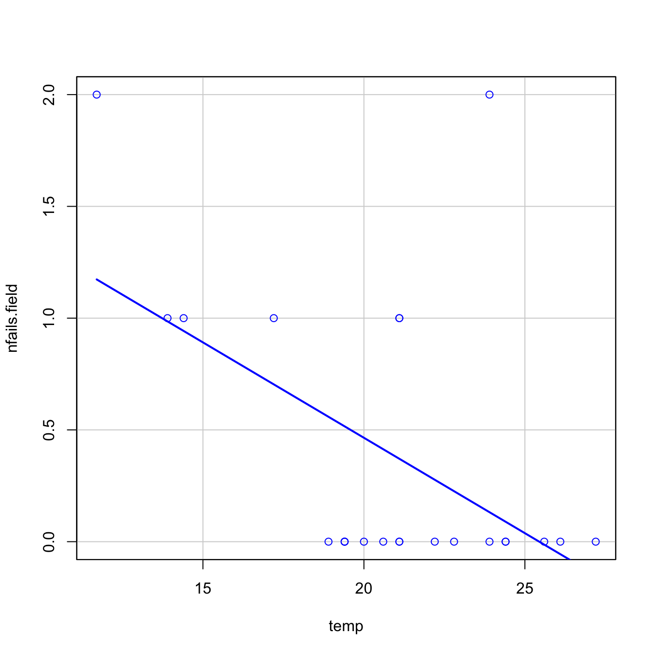
There is a fundamental problem in using linear regression for this data: the response is not continuous. As a consequence, there is no linearity and the errors around the mean are not normal (indeed, they are strongly non-normal). Let’s check this with the corresponding diagnostic plots:
# Fit linear model, and run linearity and normality diagnostics
mod <- lm(nfails.field ~ temp, data = challenger)
plot(mod, 1)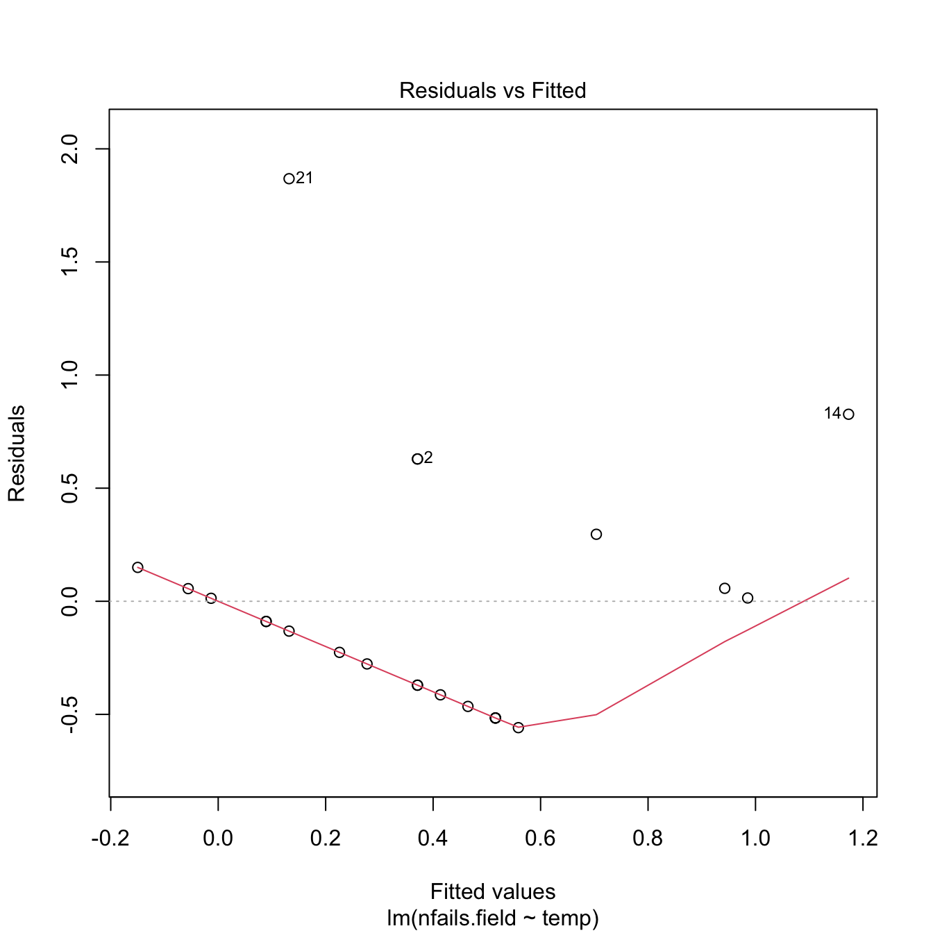
plot(mod, 2)
Although linear regression is not the appropriate tool for this data, it is able to detect the obvious difference between the two plots:
- The trend for launches with incidents is flat, hence suggesting there is no correlation on the temperature (Figure 5.3a). This was one of the arguments behind NASA’s decision to launch the rocket at a temperature of \(-0.6\) degrees Celsius.
- However, as Figure 5.3b reveals, the trend for all launches indicates a clear negative dependence between temperature and number of incidents! Think about it in this way: the minimum temperature for a launch without incidents ever recorded was above \(18\) degrees Celsius, and the Challenger was launched at \(-0.6\) without clearly knowing the effects of such low temperatures.
Along this chapter we will see the required tools for answering precisely Q1–Q4.
5.2 Model formulation and estimation
For simplicity, we first study the logistic regression and then study the general case of a generalized linear model.
5.2.1 Logistic regression
As we saw in Section 2.2, the multiple linear model described the relation between the random variables \(X_1,\ldots,X_p\) and \(Y\) by assuming a linear relation in the conditional expectation:
\[\begin{align} \mathbb{E}[Y \mid X_1=x_1,\ldots,X_p=x_p]=\beta_0+\beta_1x_1+\cdots+\beta_px_p.\tag{5.1} \end{align}\]
In addition, it made three more assumptions on the data (see Section 2.3), which resulted in the following one-line summary of the linear model:
\[\begin{align*} Y \mid (X_1=x_1,\ldots,X_p=x_p)\sim \mathcal{N}(\beta_0+\beta_1x_1+\cdots+\beta_px_p,\sigma^2). \end{align*}\]
Recall that a necessary condition for the linear model to hold is that \(Y\) is continuous, in order to satisfy the normality of the errors. Therefore, the linear model is designed for a continuous response.
The situation when \(Y\) is discrete (naturally ordered values) or categorical (non-ordered categories) requires a different treatment. The simplest situation is when \(Y\) is binary: it can only take two values, codified for convenience as \(1\) (success) and \(0\) (failure). For binary variables there is no fundamental distinction between the treatment of discrete and categorical variables. Formally, a binary variable is referred to as a Bernoulli variable:150 \(Y\sim\mathrm{Ber}(p),\) \(0\leq p\leq1\;\)151, if
\[\begin{align*} Y=\left\{\begin{array}{ll}1,&\text{with probability }p,\\0,&\text{with probability }1-p,\end{array}\right. \end{align*}\]
or, equivalently, if
\[\begin{align} \mathbb{P}[Y=y]=p^y(1-p)^{1-y},\quad y=0,1.\tag{5.2} \end{align}\]
Recall that a Bernoulli variable is completely determined by the probability \(p.\) Therefore, so are its mean and variance:
\[\begin{align*} \mathbb{E}[Y]=\mathbb{P}[Y=1]=p\quad\text{and}\quad\mathbb{V}\mathrm{ar}[Y]=p(1-p). \end{align*}\]
Assume then that \(Y\) is a Bernoulli variable and that \(X_1,\ldots,X_p\) are predictors associated with \(Y.\) The purpose in logistic regression is to model
\[\begin{align} \mathbb{E}[Y \mid X_1=x_1,\ldots,X_p=x_p]=\mathbb{P}[Y=1 \mid X_1=x_1,\ldots,X_p=x_p],\tag{5.3} \end{align}\]
that is, to model how the conditional expectation of \(Y\) or, equivalently, the conditional probability of \(Y=1,\) is changing according to particular values of the predictors. At sight of (5.1), a tempting possibility is to consider the model
\[\begin{align*} \mathbb{E}[Y \mid X_1=x_1,\ldots,X_p=x_p]=\beta_0+\beta_1x_1+\cdots+\beta_px_p=:\eta. \end{align*}\]
However, such a model will run into serious problems inevitably: negative probabilities and probabilities larger than one may happen.
A solution is to consider a link function \(g\) to encapsulate the value of \(\mathbb{E}[Y \mid X_1=x_1,\ldots,X_p=x_p]\) and map it back to \(\mathbb{R}.\) Or, alternatively, a function \(g^{-1}\) that takes \(\eta\in\mathbb{R}\) and maps it to \([0,1],\) the support of \(\mathbb{E}[Y \mid X_1=x_1,\ldots,X_p=x_p].\) There are several link functions \(g\) with associated \(g^{-1}.\) Each link generates a different model:
- Uniform link. Based on the truncation \(g^{-1}(\eta)=\eta\mathbb{1}_{\{0<\eta<1\}}+\mathbb{1}_{\{\eta\geq1\}}.\)
- Probit link. Based on the normal cdf, that is, \(g^{-1}(\eta)=\Phi(\eta).\)
- Logit link. Based on the logistic cdf:152
\[\begin{align*} g^{-1}(\eta)=\mathrm{logistic}(\eta):=\frac{e^\eta}{1+e^\eta}=\frac{1}{1+e^{-\eta}}. \end{align*}\]
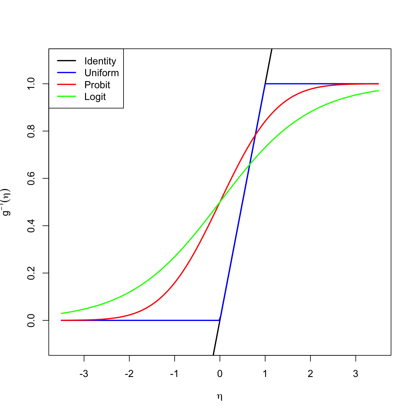
Figure 5.4: Transformations \(g^{-1}\) associated with different link functions. The transformations \(g^{-1}\) map the response of a linear regression \(\eta=\beta_0+\beta_1x_1+\cdots+\beta_px_p\) to \(\lbrack 0,1\rbrack.\)
The logistic transformation is the most employed due to its tractability, interpretability, and smoothness.153 Its inverse, \(g:[0,1]\longrightarrow\mathbb{R},\) is known as the logit function:
\[\begin{align*} \mathrm{logit}(p):=\mathrm{logistic}^{-1}(p)=\log\left(\frac{p}{1-p}\right). \end{align*}\]
In conclusion, with the logit link function we can map the domain of \(Y\) to \(\mathbb{R}\) in order to apply a linear model. The logistic model can be then equivalently stated as
\[\begin{align} \mathbb{P}[Y=1 \mid X_1=x_1,\ldots,X_p=x_p]&=\mathrm{logistic}(\eta)=\frac{1}{1+e^{-\eta}}\tag{5.4}, \end{align}\]
or as
\[\begin{align} \mathrm{logit}(\mathbb{P}[Y=1 \mid X_1=x_1,\ldots,X_p=x_p])=\eta \tag{5.5} \end{align}\]
where recall that
\[\begin{align*} \eta=\beta_0+\beta_1x_1+\cdots+\beta_px_p. \end{align*}\]
There is a clear interpretation of the role of the linear predictor \(\eta\) in (5.4) when we come back to (5.3):
- If \(\eta=0,\) then \(\mathbb{P}[Y=1 \mid X_1=x_1,\ldots,X_p=x_p]=\frac{1}{2}\) (\(Y=1\) and \(Y=0\) are equally likely).
- If \(\eta<0,\) then \(\mathbb{P}[Y=1 \mid X_1=x_1,\ldots,X_p=x_p]<\frac{1}{2}\) (\(Y=1\) is less likely).
- If \(\eta>0,\) then \(\mathbb{P}[Y=1 \mid X_1=x_1,\ldots,X_p=x_p]>\frac{1}{2}\) (\(Y=1\) is more likely).
To be more precise on the interpretation of the coefficients we need to introduce the odds. The odds is an equivalent way of expressing the distribution of probabilities in a binary variable \(Y.\) Instead of using \(p\) to characterize the distribution of \(Y,\) we can use
\[\begin{align} \mathrm{odds}(Y):=\frac{p}{1-p}=\frac{\mathbb{P}[Y=1]}{\mathbb{P}[Y=0]}.\tag{5.6} \end{align}\]
The odds is thus the ratio between the probability of success and the probability of failure.154 It is extensively used in betting.155 due to its better interpretability156 Conversely, if the odds of \(Y\) is given, we can easily know what is the probability of success \(p,\) using the inverse of (5.6):157
\[\begin{align*} p=\mathbb{P}[Y=1]=\frac{\text{odds}(Y)}{1+\text{odds}(Y)}. \end{align*}\]
Recall that the odds is a number in \([0,+\infty].\) The \(0\) and \(+\infty\) values are attained for \(p=0\) and \(p=1,\) respectively. The log-odds (or logit) is a number in \([-\infty,+\infty].\)
We can rewrite (5.4) in terms of the odds (5.6)158 so we get:
\[\begin{align} \mathrm{odds}(Y \mid X_1=x_1,\ldots,X_p=x_p)=e^{\eta}=e^{\beta_0}e^{\beta_1x_1}\cdots e^{\beta_px_p}.\tag{5.7} \end{align}\]
Alternatively, taking logarithms, we have the log-odds (or logit)
\[\begin{align} \log(\mathrm{odds}(Y \mid X_1=x_1,\ldots,X_p=x_p))=\beta_0+\beta_1x_1+\cdots+\beta_px_p.\tag{5.8} \end{align}\]
The conditional log-odds (5.8) plays the role of the conditional mean for multiple linear regression. Therefore, we have an analogous interpretation for the coefficients:
- \(\beta_0\): is the log-odds when \(X_1=\cdots=X_p=0.\)
- \(\beta_j,\) \(1\leq j\leq p\): is the additive increment of the log-odds for an increment of one unit in \(X_j=x_j,\) provided that the remaining variables \(X_1,\ldots,X_{j-1},X_{j+1},\ldots,X_p\) do not change.
The log-odds is not as easy to interpret as the odds. For that reason, an equivalent way of interpreting the coefficients, this time based on (5.7), is:
- \(e^{\beta_0}\): is the odds when \(X_1=\cdots=X_p=0.\)
- \(e^{\beta_j},\) \(1\leq j\leq p\): is the multiplicative increment of the odds for an increment of one unit in \(X_j=x_j,\) provided that the remaining variables \(X_1,\ldots,X_{j-1},X_{j+1},\ldots,X_p\) do not change. If the increment in \(X_j\) is of \(r\) units, then the multiplicative increment in the odds is \((e^{\beta_j})^r.\)
As a consequence of this last interpretation, we have:
5.2.1.1 Case study application
In the Challenger case study we used fail.field as an indicator of whether “there was at least an incident with the O-rings” (1 = yes, 0 = no). Let’s see if the temperature was associated with O-ring incidents (Q1). For that, we compute the logistic regression of fail.field on temp and we plot the fitted logistic curve.
# Logistic regression: computed with glm and family = "binomial"
nasa <- glm(fail.field ~ temp, family = "binomial", data = challenger)
nasa
##
## Call:  glm(formula = fail.field ~ temp, family = "binomial", data = challenger)
##
## Coefficients:
## (Intercept)         temp
##      7.5837      -0.4166
##
## Degrees of Freedom: 22 Total (i.e. Null);  21 Residual
## Null Deviance:       28.27
## Residual Deviance: 20.33     AIC: 24.33

# Plot data
plot(challenger$temp, challenger$fail.field, xlim = c(-1, 30),
     xlab = "Temperature", ylab = "Incident probability")

# Draw the fitted logistic curve
x <- seq(-1, 30, l = 200)
eta <- nasa$coefficients[1] + nasa$coefficients[2] * x
y <- 1 / (1 + exp(-eta))
lines(x, y, col = 2, lwd = 2)

# The Challenger
points(-0.6, 1, pch = 16)
text(-0.6, 1, labels = "Challenger", pos = 4)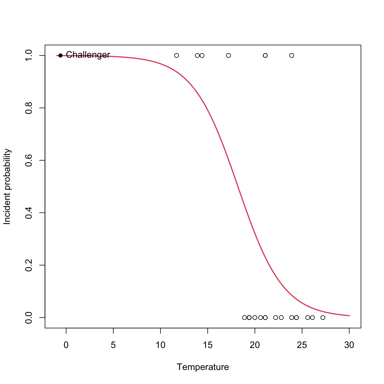
At the sight of this curve and the summary it seems that the temperature was affecting the probability of an O-ring incident (Q1). Let’s quantify this statement and answer Q2 by looking to the coefficients of the model:
# Exponentiated coefficients ("odds ratios")
exp(coef(nasa))
##  (Intercept)         temp
## 1965.9743592    0.6592539
The exponentials of the estimated coefficients are:
- \(e^{\hat\beta_0}=1965.974.\) This means that, when the temperature is zero, the fitted odds is \(1965.974,\) so the (estimated) probability of having an incident (\(Y=1\)) is \(1965.974\) times larger than the probability of not having an incident (\(Y=0\)). Or, in other words, the probability of having an incident at temperature zero is \(\frac{1965.974}{1965.974+1}=0.999.\)
- \(e^{\hat\beta_1}=0.659.\) This means that each Celsius degree increment on the temperature multiplies the fitted odds by a factor of \(0.659\approx\frac{2}{3},\) hence reducing it.
However, for the moment we cannot say whether these findings are significant or are just an artifact of the randomness of the data, since we do not have information on the variability of the estimates of \(\boldsymbol{\beta}.\) We will need inference for that.
5.2.1.2 Estimation by maximum likelihood
The estimation of \(\boldsymbol{\beta}\) from a sample \(\{(\mathbf{x}_i,Y_i)\}_{i=1}^n\;\)159 is done by Maximum Likelihood Estimation (MLE). As it can be seen in Appendix B, in the linear model, under the assumptions mentioned in Section 2.3, MLE is equivalent to least squares estimation. In the logistic model, we assume that160
\[\begin{align*} Y_i\mid (X_{1}=x_{i1},\ldots,X_{p}=x_{ip})\sim \mathrm{Ber}(\mathrm{logistic}(\eta_i)),\quad i=1,\ldots,n, \end{align*}\]
where \(\eta_i:=\beta_0+\beta_1x_{i1}+\cdots+\beta_px_{ip}.\) Denoting \(p_i(\boldsymbol{\beta}):=\mathrm{logistic}(\eta_i),\) the log-likelihood of \(\boldsymbol{\beta}\) is
\[\begin{align} \ell(\boldsymbol{\beta})&=\log\left(\prod_{i=1}^np_i(\boldsymbol{\beta})^{Y_i}(1-p_i(\boldsymbol{\beta}))^{1-Y_i}\right)\nonumber\\ &=\sum_{i=1}^n\left[Y_i\log(p_i(\boldsymbol{\beta}))+(1-Y_i)\log(1-p_i(\boldsymbol{\beta}))\right].\tag{5.9} \end{align}\]
The ML estimate of \(\boldsymbol{\beta}\) is
\[\begin{align*} \hat{\boldsymbol{\beta}}:=\arg\max_{\boldsymbol{\beta}\in\mathbb{R}^{p+1}}\ell(\boldsymbol{\beta}). \end{align*}\]
Unfortunately, due to the nonlinearity of (5.9), there is no explicit expression for \(\hat{\boldsymbol{\beta}}\) and it has to be obtained numerically by means of an iterative procedure. We will see that with more detail in the next section. Just be aware that this iterative procedure may fail to converge in low sample size situations with perfect classification, where the likelihood might be numerically unstable.
Figure 5.5: The logistic regression fit and its dependence on \(\beta_0\) (horizontal displacement) and \(\beta_1\) (steepness of the curve). Recall the effect of the sign of \(\beta_1\) in the curve: if positive, the logistic curve has an ‘s’ form; if negative, the form is a reflected ‘s’. Application available here.
Figure 5.5 shows how the log-likelihood changes with respect to the values for \((\beta_0,\beta_1)\) in three data patterns. The data of the illustration has been generated with the next chunk of code.
# Data
set.seed(987204452)
x <- rnorm(50, sd = 1.5)
y1 <- -0.5 + 3 * x
y2 <- 0.5 - 2 * x
y3 <- -2 + 5 * x
y1 <- rbinom(50, size = 1, prob = 1 / (1 + exp(-y1)))
y2 <- rbinom(50, size = 1, prob = 1 / (1 + exp(-y2)))
y3 <- rbinom(50, size = 1, prob = 1 / (1 + exp(-y3)))

# Data
data_mle <- data.frame(x = x, y1 = y1, y2 = y2, y3 = y3)
For fitting a logistic model we employ glm, which has the syntax glm(formula = response ~ predictor, family = "binomial", data = data), where response is a binary variable. Note that family = "binomial" is referring to the fact that the response is a binomial variable (since it is a Bernoulli). Let’s check that indeed the coefficients given by glm are the ones that maximize the likelihood given in the animation of Figure 5.5. We do so for y1 ~ x.
# Call glm
mod <- glm(y1 ~ x, family = "binomial", data = data_mle)
mod$coefficients
## (Intercept)           x
##  -0.9464403   2.8566464

# -loglik(beta)
minus_log_lik <- function(beta) {
  p <- 1 / (1 + exp(-(beta[1] + beta[2] * x)))
  -sum(y1 * log(p) + (1 - y1) * log(1 - p))
}

# Optimization using as starting values beta = c(0, 0)
opt <- optim(par = c(0, 0), fn = minus_log_lik)
opt
## $par
## [1] -0.9464609  2.8558362
##
## $value
## [1] 11.5585
##
## $counts
## function gradient
##       63       NA
##
## $convergence
## [1] 0
##
## $message
## NULL

# Visualization of the negative log-likelihood surface
beta0 <- seq(-4, 2, l = 200)
beta1 <- seq(0, 8, l = 200)
L <- matrix(nrow = length(beta0), ncol = length(beta1))
for (i in seq_along(beta0)) {
  for (j in seq_along(beta1)) {
    L[i, j] <- minus_log_lik(c(beta0[i], beta1[j]))
  }
}

# Log-spaced levels concentrate the contour density around the minimum of L
n_lev <- 30
lev_breaks <- 10^seq(log10(min(L)), log10(max(L)), length.out = n_lev + 1)
lev_lines <- lev_breaks[-c(1, length(lev_breaks))]

image(beta0, beta1, L, breaks = lev_breaks,
      col = viridis::viridis(n_lev, direction = -1),
      xlab = expression(beta[0]), ylab = expression(beta[1]), las = 1)
contour(beta0, beta1, L, levels = lev_lines, labels = round(lev_lines),
        add = TRUE, labcex = 0.5, lwd = 0.4)
points(mod$coefficients[1], mod$coefficients[2], col = 2, pch = 16)
points(opt$par[1], opt$par[2], col = 4)
Figure 5.6: Negative log-likelihood surface \(-\ell(\beta_0,\beta_1)\) and its global minimum \((\hat\beta_0,\hat\beta_1),\) which corresponds to the maximum likelihood estimator.
Exercise 5.1 For the regressions y2 ~ x and y3 ~ x, do the following:
5.2.2 General case
The same idea we used in logistic regression, namely transforming the conditional expectation of \(Y\) into something that can be modeled by a linear model (that is, a quantity that lives in \(\mathbb{R}\)), can be generalized. This raises the family of generalized linear models, which extends the linear model to different kinds of response variables and provides a convenient parametric framework.
The first ingredient is a link function \(g,\) that is monotonic and differentiable, which is going to produce a transformed expectation161 to be modeled by a linear combination of the predictors:
\[\begin{align*} g\left(\mathbb{E}[Y \mid X_1=x_1,\ldots,X_p=x_p]\right)=\eta \end{align*}\]
or, equivalently,
\[\begin{align*} \mathbb{E}[Y \mid X_1=x_1,\ldots,X_p=x_p]&=g^{-1}(\eta), \end{align*}\]
where
\[\begin{align*} \eta:=\beta_0+\beta_1x_1+\cdots+\beta_px_p \end{align*}\]
is the linear predictor.
The second ingredient of generalized linear models is a distribution for \(Y \mid (X_1,\ldots,X_p),\) just as the linear model assumes normality or the logistic model assumes a Bernoulli random variable. Thus, we have two linked generalizations with respect to the usual linear model:
- The conditional mean may be modeled by a transformation \(g^{-1}\) of the linear predictor \(\eta.\)
- The distribution of \(Y \mid (X_1,\ldots,X_p)\) may be different from the normal.
Generalized linear models are intimately related with the exponential family,162 163 which is the family of distributions with pdf expressible as
\[\begin{align} f(y;\theta,\phi)=\exp\left\{\frac{y\theta-b(\theta)}{a(\phi)}+c(y,\phi)\right\},\tag{5.10} \end{align}\]
where \(a(\cdot),\) \(b(\cdot),\) and \(c(\cdot,\cdot)\) are specific functions. If \(Y\) has the pdf (5.10), then we write \(Y\sim\mathrm{E}(\theta,\phi,a,b,c).\) If the scale parameter \(\phi\) is known, this is an exponential family with canonical parameter \(\theta\) (if \(\phi\) is unknown, then it may or may not be a two-parameter exponential family).
Distributions from the exponential family have some nice properties. Importantly, if \(Y\sim\mathrm{E}(\theta,\phi,a,b,c),\) then
\[\begin{align} \mu:=\mathbb{E}[Y]=b'(\theta),\quad \sigma^2:=\mathbb{V}\mathrm{ar}[Y]=b''(\theta)a(\phi).\tag{5.11} \end{align}\]
The canonical link function is the function \(g\) that transforms \(\mu=b'(\theta)\) into the canonical parameter \(\theta\). For \(\mathrm{E}(\theta,\phi,a,b,c),\) this happens if
\[\begin{align} \theta=g(\mu) \tag{5.12} \end{align}\]
or, more explicitly due to (5.11), if
\[\begin{align} g(\mu)=(b')^{-1}(\mu). \tag{5.13} \end{align}\]
In the case of canonical link function, the one-line summary of the generalized linear model is (independence is implicit)
\[\begin{align} Y \mid (X_1=x_1,\ldots,X_p=x_p)\sim\mathrm{E}(\eta,\phi,a,b,c).\tag{5.14} \end{align}\]
Expression (5.14) gives insight on what a generalized linear model does:
- Select a member of the exponential family in (5.10) for modeling \(Y.\)
- The canonical link function \(g\) is \(g(\mu)=(b')^{-1}(\mu).\) In this case, \(\theta=g(\mu).\)
- The generalized linear model associated with the member of the exponential family and \(g\) models the conditional \(\theta,\) given \(X_1,\ldots,X_n,\) by means of the linear predictor \(\eta.\) This is equivalent to modeling the conditional \(\mu\) by means of \(g^{-1}(\eta).\)
The linear model arises as a particular case of (5.14) with
\[\begin{align*} a(\phi)=\phi,\quad b(\theta)=\frac{\theta^2}{2},\quad c(y,\phi)=-\frac{1}{2}\left\{\frac{y^2}{\phi}+\log(2\pi\phi)\right\}, \end{align*}\]
and scale parameter \(\phi=\sigma^2.\) In this case, \(\mu=\theta\) and the canonical link function \(g\) is the identity.
Exercise 5.2 Show that the normal, Bernoulli, exponential, and Poisson distributions are members of the exponential family. For that, express their pdfs in terms of (5.10) and identify who is \(\theta\) and \(\phi.\)
Exercise 5.3 Show that the binomial and gamma (which includes exponential and chi-squared) distributions are members of the exponential family. For that, express their pdfs in terms of (5.10) and identify who is \(\theta\) and \(\phi.\)
The following table lists some useful generalized linear models. Recall that the linear and logistic models of Sections 2.2.3 and 5.2.1 are obtained from the first and second rows, respectively.
| Support of \(Y\) | Generating distribution | Link \(g(\mu)\) | Expectation \(g^{-1}(\eta)\) | Scale \(\phi\) | Distribution of \(Y \mid \mathbf{X}=\mathbf{x}\) |
|---|---|---|---|---|---|
| \(\mathbb{R}\) | \(\mathcal{N}(\mu,\sigma^2)\) | \(\mu\) | \(\eta\) | \(\sigma^2\) | \(\mathcal{N}(\eta,\sigma^2)\) |
| \(\{0,1\}\) | \(\mathrm{Ber}(p)\) | \(\mathrm{logit}(\mu)\) | \(\mathrm{logistic}(\eta)\) | \(1\) | \(\mathrm{Ber}\left(\mathrm{logistic}(\eta)\right)\) |
| \(\{0,\ldots,N\}\) | \(\mathrm{B}(N,p)\) | \(\log\left(\frac{\mu}{N-\mu}\right)\) | \(N\cdot\mathrm{logistic}(\eta)\) | \(1\) | \(\mathrm{B}(N,\mathrm{logistic}(\eta))\) |
| \(\{0,1,\ldots\}\) | \(\mathrm{Pois}(\lambda)\) | \(\log(\mu)\) | \(e^\eta\) | \(1\) | \(\mathrm{Pois}(e^{\eta})\) |
| \((0,\infty)\) | \(\Gamma(a,\nu)\;\)164 | \(-\frac{1}{\mu}\) | \(-\frac{1}{\eta}\) | \(\frac{1}{\nu}\) | \(\Gamma(-\eta \nu,\nu)\;\)165 |
Exercise 5.4 Obtain the canonical link function for the exponential distribution \(\mathrm{Exp}(\lambda).\) What is the scale parameter? What is the distribution of \(Y \mid (X_1=x_1,\ldots,X_p=x_p)\) in such model?
5.2.2.1 Poisson regression
Poisson regression is usually employed for modeling count data that arises from the recording of the frequencies of a certain phenomenon. It considers that
\[\begin{align*} Y \mid (X_1=x_1,\ldots,X_p=x_p)\sim\mathrm{Pois}(e^{\eta}), \end{align*}\]
that is,
\[\begin{align} \mathbb{E}[Y \mid X_1=x_1,\ldots,X_p=x_p]&=\lambda(Y \mid X_1=x_1,\ldots,X_p=x_p)\nonumber\\ &=e^{\beta_0+\beta_1x_1+\cdots+\beta_px_p}.\tag{5.15} \end{align}\]
Let’s see how to apply a Poisson regression. For that aim we consider the species (download) dataset. The goal is to analyze whether the Biomass and the pH (a factor) of the terrain are influential on the number of Species. Incidentally, it will serve to illustrate that the use of factors within glm is completely analogous to what we did with lm.
# Read data
species <- read.table("species.txt", header = TRUE)
species$pH <- as.factor(species$pH)
# Plot data
plot(Species ~ Biomass, data = species, col = as.numeric(pH))
legend("topright", legend = c("High pH", "Medium pH", "Low pH"),
       col = c(1, 3, 2), lwd = 2) # colors according to as.numeric(pH)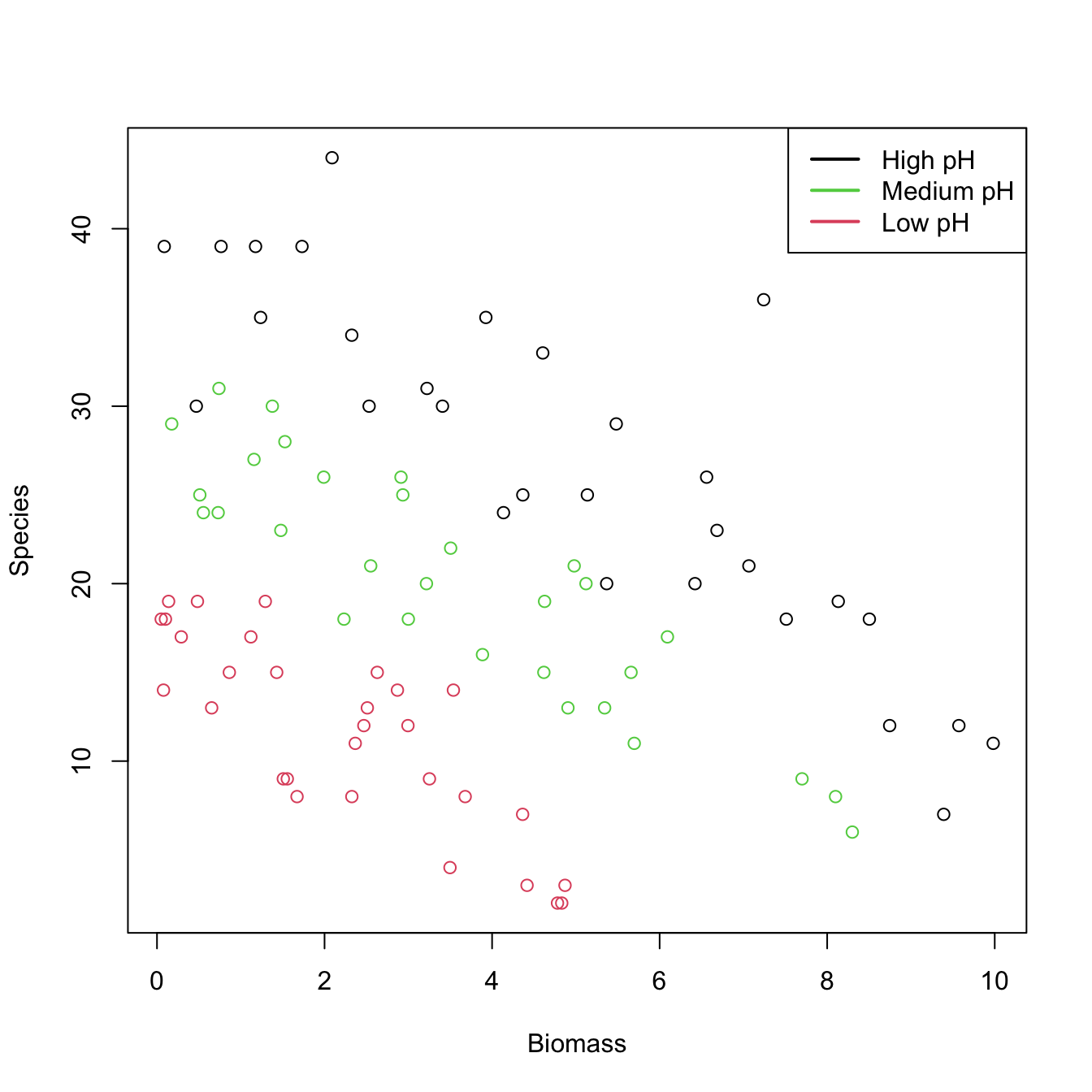
# Fit Poisson regression
species1 <- glm(Species ~ ., data = species, family = poisson)
summary(species1)
##
## Call:
## glm(formula = Species ~ ., family = poisson, data = species)
##
## Coefficients:
##             Estimate Std. Error z value Pr(>|z|)
## (Intercept)  3.84894    0.05281  72.885  < 2e-16 ***
## pHlow       -1.13639    0.06720 -16.910  < 2e-16 ***
## pHmed       -0.44516    0.05486  -8.114 4.88e-16 ***
## Biomass     -0.12756    0.01014 -12.579  < 2e-16 ***
## ---
## Signif. codes:  0 '***' 0.001 '**' 0.01 '*' 0.05 '.' 0.1 ' ' 1
##
## (Dispersion parameter for poisson family taken to be 1)
##
##     Null deviance: 452.346  on 89  degrees of freedom
## Residual deviance:  99.242  on 86  degrees of freedom
## AIC: 526.43
##
## Number of Fisher Scoring iterations: 4
# Took 4 iterations of the IRLS

# Interpretation of the coefficients:
exp(species1$coefficients)
## (Intercept)       pHlow       pHmed     Biomass
##  46.9433686   0.3209744   0.6407222   0.8802418
# - 46.9433 is the average number of species when Biomass = 0 and the pH is high
# - For each increment in one unit in Biomass, the number of species decreases
#   by a factor of 0.88 (12% reduction)
# - If pH decreases to med (low), then the number of species decreases by a factor
#   of 0.6407 (0.3209)

# With interactions
species2 <- glm(Species ~ Biomass * pH, data = species, family = poisson)
summary(species2)
##
## Call:
## glm(formula = Species ~ Biomass * pH, family = poisson, data = species)
##
## Coefficients:
##               Estimate Std. Error z value Pr(>|z|)
## (Intercept)    3.76812    0.06153  61.240  < 2e-16 ***
## Biomass       -0.10713    0.01249  -8.577  < 2e-16 ***
## pHlow         -0.81557    0.10284  -7.931 2.18e-15 ***
## pHmed         -0.33146    0.09217  -3.596 0.000323 ***
## Biomass:pHlow -0.15503    0.04003  -3.873 0.000108 ***
## Biomass:pHmed -0.03189    0.02308  -1.382 0.166954
## ---
## Signif. codes:  0 '***' 0.001 '**' 0.01 '*' 0.05 '.' 0.1 ' ' 1
##
## (Dispersion parameter for poisson family taken to be 1)
##
##     Null deviance: 452.346  on 89  degrees of freedom
## Residual deviance:  83.201  on 84  degrees of freedom
## AIC: 514.39
##
## Number of Fisher Scoring iterations: 4
exp(species2$coefficients)
##   (Intercept)       Biomass         pHlow         pHmed Biomass:pHlow Biomass:pHmed
##    43.2987424     0.8984091     0.4423865     0.7178730     0.8563910     0.9686112
# - If pH decreases to med (low), then the effect of the biomass in the number
#   of species decreases by a factor of 0.9686 (0.8564). The higher the pH, the
#   stronger the effect of the Biomass in Species

# Draw fits
plot(Species ~ Biomass, data = species, col = as.numeric(pH))
legend("topright", legend = c("High pH", "Medium pH", "Low pH"),
       col = c(1, 3, 2), lwd = 2) # colors according to as.numeric(pH)

# Without interactions
bio <- seq(0, 10, l = 100)
z <- species1$coefficients[1] + species1$coefficients[4] * bio
lines(bio, exp(z), col = 1)
lines(bio, exp(species1$coefficients[2] + z), col = 2)
lines(bio, exp(species1$coefficients[3] + z), col = 3)

# With interactions seems to provide a significant improvement
bio <- seq(0, 10, l = 100)
z <- species2$coefficients[1] + species2$coefficients[2] * bio
lines(bio, exp(z), col = 1, lty = 2)
lines(bio, exp(species2$coefficients[3] + species2$coefficients[5] * bio + z),
      col = 2, lty = 2)
lines(bio, exp(species2$coefficients[4] + species2$coefficients[6] * bio + z),
      col = 3, lty = 2)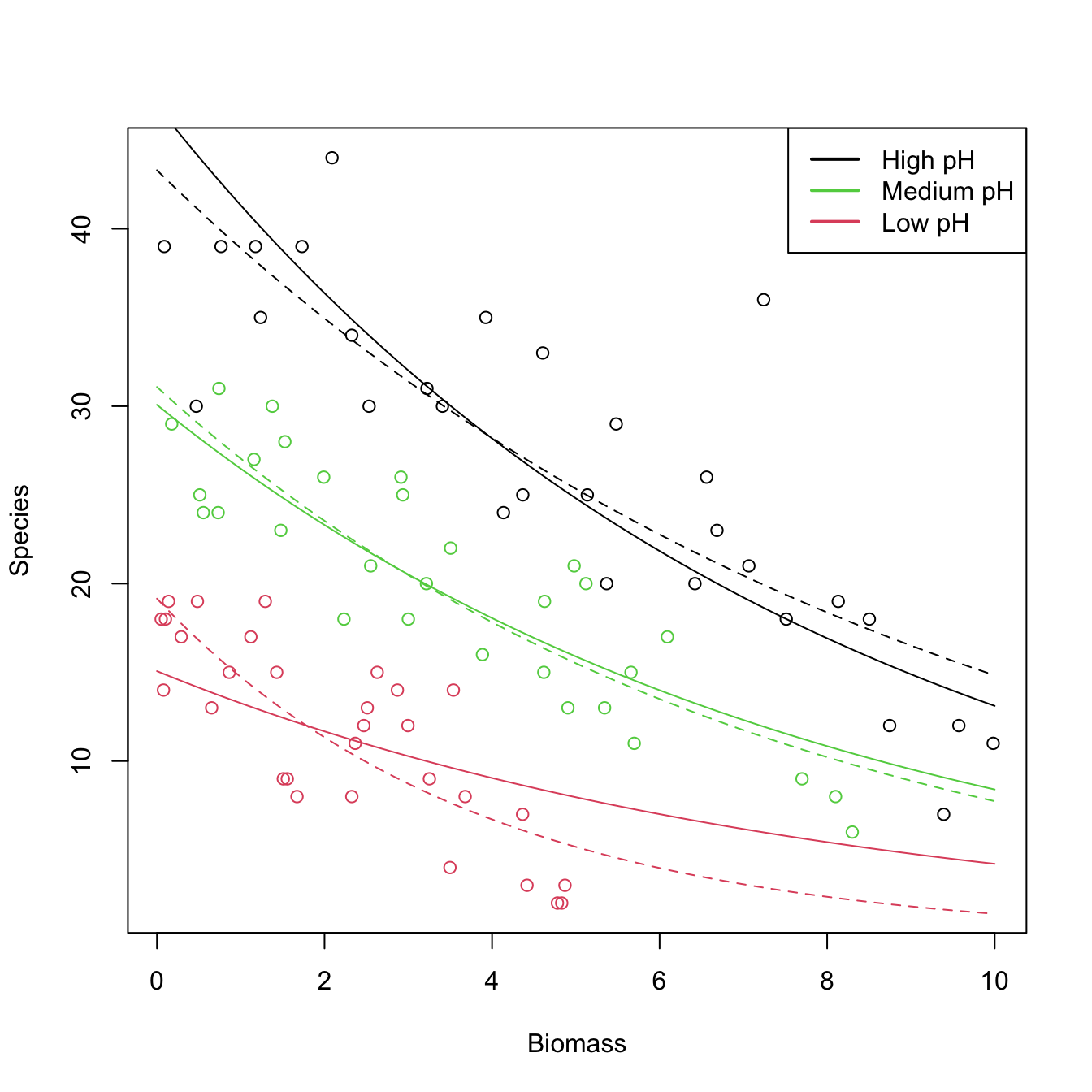
Exercise 5.5 For the challenger dataset, do the following:
- Do a Poisson regression of the total number of incidents,
nfails.field + nfails.nozzle, ontemp. - Plot the data and the fitted Poisson regression curve.
- Predict the expected number of incidents at temperatures \(-0.6\) and \(11.67.\)
5.2.2.2 Binomial regression
Binomial regression is an extension of logistic regression that allows us to model discrete responses \(Y\) in \(\{0,1,\ldots,N\},\) where \(N\) is fixed. In its most vanilla version, it considers the model
\[\begin{align} Y \mid (X_1=x_1,\ldots,X_p=x_p)\sim\mathrm{B}(N,\mathrm{logistic}(\eta)),\tag{5.16} \end{align}\]
that is,
\[\begin{align} \mathbb{E}[Y \mid X_1=x_1,\ldots,X_p=x_p]=N\cdot\mathrm{logistic}(\eta).\tag{5.17} \end{align}\]
Comparing (5.17) with (5.4), it is clear that the logistic regression is a particular case with \(N=1.\) The interpretation of the coefficients is therefore clear from the interpretation of (5.4), given that \(\mathrm{logistic}(\eta)\) models the probability of success of each of the \(N\) experiments of the binomial \(\mathrm{B}(N,\mathrm{logistic}(\eta)).\)
The extra flexibility that binomial regression has offers interesting applications. First, we can use (5.16) as an approach to model proportions166 \(Y/N\in[0,1].\) In this case, (5.17) becomes167
\[\begin{align*} \mathbb{E}[Y/N \mid X_1=x_1,\ldots,X_p=x_p]=\mathrm{logistic}(\eta). \end{align*}\]
Second, we can let \(N\) be dependent on the predictors to accommodate group structures, perhaps the most common usage of binomial regression:
\[\begin{align} Y \mid \mathbf{X}=\mathbf{x}\sim\mathrm{B}(N_\mathbf{x},\mathrm{logistic}(\eta)),\tag{5.18} \end{align}\]
where the size of the binomial distribution, \(N_\mathbf{x},\) depends on the values of the predictors. For example, imagine that the predictors are two quantitative variables and two dummy variables encoding three categories. Then \(\mathbf{X}=(X_1,X_2, D_1,D_2)^\top\) and \(\mathbf{x}=(x_1,x_2, d_1,d_2)^\top.\) In this case, \(N_\mathbf{x}\) could for example take the form
\[\begin{align*} N_\mathbf{x}=\begin{cases} 30,&d_1=0,d_2=0,\\ 25,&d_1=1,d_2=0,\\ 50,&d_1=0,d_2=1, \end{cases} \end{align*}\]
that is, we have a different number of experiments on each category, and we want to model the number (or, equivalently, the proportion) of successes for each one, also taking into account the effects of other qualitative variables. This is a very common situation in practice, when one encounters the sample version of (5.18):
\[\begin{align} Y_i\mid \mathbf{X}_i=\mathbf{x}_i\sim\mathrm{B}(N_i,\mathrm{logistic}(\eta_i)),\quad i=1,\ldots,n.\tag{5.19} \end{align}\]
Let’s see an example of binomial regression that illustrates the particular usage of glm() in this case. The example is a data application from Wood (2006) featuring different binomial sizes. It employs the heart (download) dataset. The goal is to investigate whether the level of creatinine kinase level present in the blood, ck, is a good diagnostic for determining if a patient is likely to have a future heart attack. The number of patients that did not have a heart attack (ok) and that had a heart attack (ha) was established after ck was measured. In total, there are \(226\) patients that have been aggregated into \(n=12\;\)168 categories of different sizes that have been created according to the average level of ck. Table 5.2 shows the data.
# Read data
heart <- read.table("heart.txt", header = TRUE)

# Sizes for each observation (Ni's)
heart$Ni <- heart$ok + heart$ha

# Proportions of patients with heart attacks
heart$prop <- heart$ha / (heart$ha + heart$ok)| ck | ha | ok | Ni | prop |
|---|---|---|---|---|
| 20 | 2 | 88 | 90 | 0.022 |
| 60 | 13 | 26 | 39 | 0.333 |
| 100 | 30 | 8 | 38 | 0.789 |
| 140 | 30 | 5 | 35 | 0.857 |
| 180 | 21 | 0 | 21 | 1.000 |
| 220 | 19 | 1 | 20 | 0.950 |
| 260 | 18 | 1 | 19 | 0.947 |
| 300 | 13 | 1 | 14 | 0.929 |
| 340 | 19 | 1 | 20 | 0.950 |
| 380 | 15 | 0 | 15 | 1.000 |
| 420 | 7 | 0 | 7 | 1.000 |
| 460 | 8 | 0 | 8 | 1.000 |
# Plot of proportions versus ck: twelve observations, each requiring
# Ni patients to determine the proportion
plot(heart$ck, heart$prop, xlab = "Creatinine kinase level",
     ylab = "Proportion of heart attacks")

# Fit binomial regression: recall the cbind() to pass the number of successes
# and failures
heart1 <- glm(cbind(ha, ok) ~ ck, family = binomial, data = heart)
summary(heart1)
##
## Call:
## glm(formula = cbind(ha, ok) ~ ck, family = binomial, data = heart)
##
## Coefficients:
##              Estimate Std. Error z value Pr(>|z|)
## (Intercept) -2.758358   0.336696  -8.192 2.56e-16 ***
## ck           0.031244   0.003619   8.633  < 2e-16 ***
## ---
## Signif. codes:  0 '***' 0.001 '**' 0.01 '*' 0.05 '.' 0.1 ' ' 1
##
## (Dispersion parameter for binomial family taken to be 1)
##
##     Null deviance: 271.712  on 11  degrees of freedom
## Residual deviance:  36.929  on 10  degrees of freedom
## AIC: 62.334
##
## Number of Fisher Scoring iterations: 6

# Alternatively: put proportions as responses, but then it is required to
# inform about the binomial size of each observation
heart1 <- glm(prop ~ ck, family = binomial, data = heart, weights = Ni)
summary(heart1)
##
## Call:
## glm(formula = prop ~ ck, family = binomial, data = heart, weights = Ni)
##
## Coefficients:
##              Estimate Std. Error z value Pr(>|z|)
## (Intercept) -2.758358   0.336696  -8.192 2.56e-16 ***
## ck           0.031244   0.003619   8.633  < 2e-16 ***
## ---
## Signif. codes:  0 '***' 0.001 '**' 0.01 '*' 0.05 '.' 0.1 ' ' 1
##
## (Dispersion parameter for binomial family taken to be 1)
##
##     Null deviance: 271.712  on 11  degrees of freedom
## Residual deviance:  36.929  on 10  degrees of freedom
## AIC: 62.334
##
## Number of Fisher Scoring iterations: 6

# Add fitted line
ck <- 0:500
newdata <- data.frame(ck = ck)
logistic <- function(eta) 1 / (1 + exp(-eta))
lines(ck, logistic(cbind(1, ck) %*% heart1$coefficients))

# It seems that a polynomial fit could better capture the "wiggly" pattern
# of the data
heart2 <- glm(prop ~ poly(ck, 2, raw = TRUE), family = binomial, data = heart,
              weights = Ni)
heart3 <- glm(prop ~ poly(ck, 3, raw = TRUE), family = binomial, data = heart,
              weights = Ni)
heart4 <- glm(prop ~ poly(ck, 4, raw = TRUE), family = binomial, data = heart,
              weights = Ni)

# Best fit given by heart3
BIC(heart1, heart2, heart3, heart4)
##        df      BIC
## heart1  2 63.30371
## heart2  3 44.27018
## heart3  4 35.59736
## heart4  5 37.96360
summary(heart3)
##
## Call:
## glm(formula = prop ~ poly(ck, 3, raw = TRUE), family = binomial,
##     data = heart, weights = Ni)
##
## Coefficients:
##                            Estimate Std. Error z value Pr(>|z|)
## (Intercept)              -5.786e+00  9.268e-01  -6.243 4.30e-10 ***
## poly(ck, 3, raw = TRUE)1  1.102e-01  2.139e-02   5.153 2.57e-07 ***
## poly(ck, 3, raw = TRUE)2 -4.649e-04  1.381e-04  -3.367  0.00076 ***
## poly(ck, 3, raw = TRUE)3  6.448e-07  2.544e-07   2.535  0.01125 *
## ---
## Signif. codes:  0 '***' 0.001 '**' 0.01 '*' 0.05 '.' 0.1 ' ' 1
##
## (Dispersion parameter for binomial family taken to be 1)
##
##     Null deviance: 271.7124  on 11  degrees of freedom
## Residual deviance:   4.2525  on  8  degrees of freedom
## AIC: 33.658
##
## Number of Fisher Scoring iterations: 6

# All fits together
lines(ck, logistic(cbind(1, poly(ck, 2, raw = TRUE)) %*% heart2$coefficients),
      col = 2)
lines(ck, logistic(cbind(1, poly(ck, 3, raw = TRUE)) %*% heart3$coefficients),
      col = 3)
lines(ck, logistic(cbind(1, poly(ck, 4, raw = TRUE)) %*% heart4$coefficients),
      col = 4)
legend("bottomright", legend = c("Linear", "Quadratic", "Cubic", "Quartic"),
       col = 1:4, lwd = 2)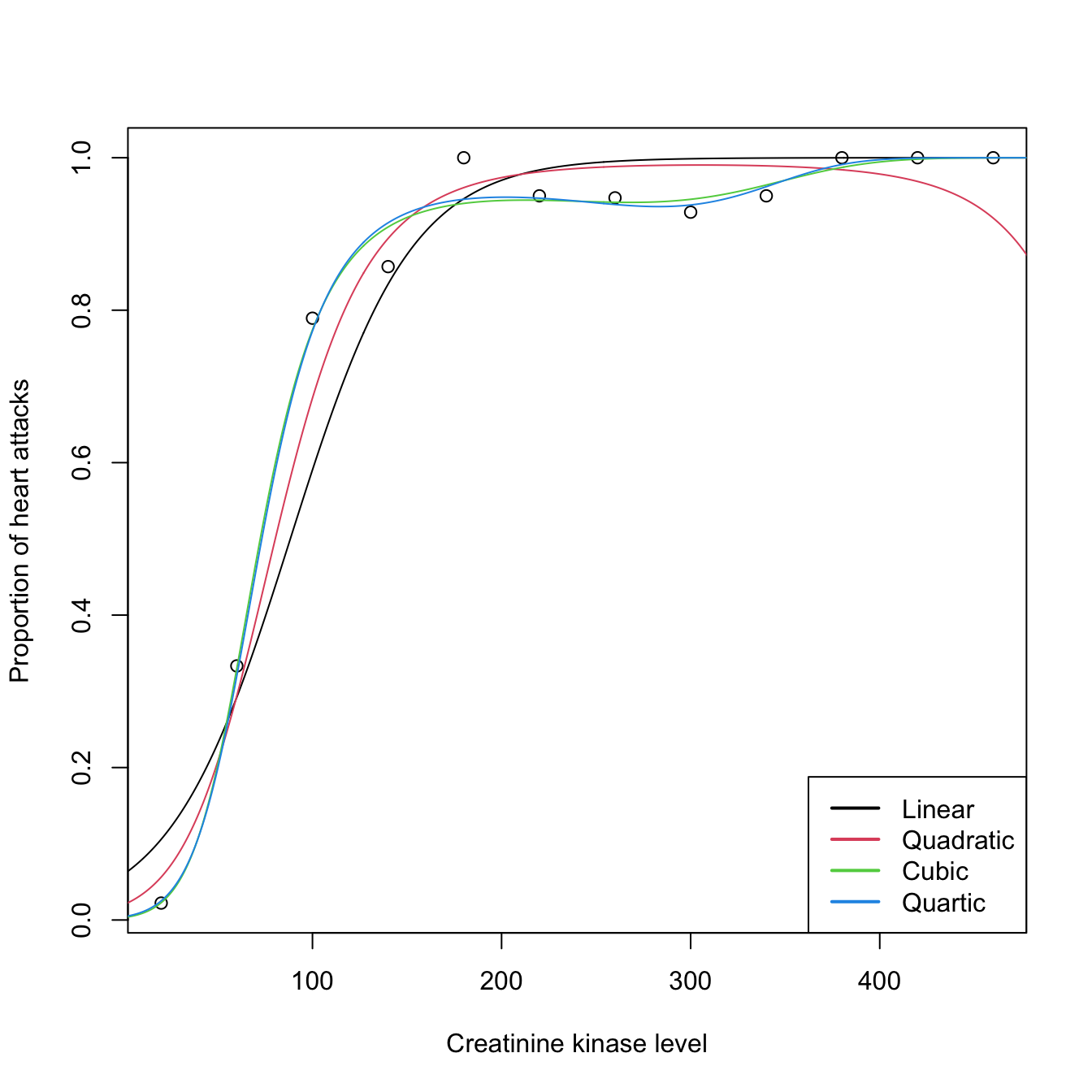
5.2.2.3 Estimation by maximum likelihood
The estimation of \(\boldsymbol{\beta}\) by MLE can be done in a unified framework, for all generalized linear models, thanks to the exponential family (5.10). Given \(\{(\mathbf{x}_i,Y_i)\}_{i=1}^n,\)169 and employing a canonical link function (5.13), we have that
\[\begin{align*} Y_i\mid (X_1=x_{i1},\ldots,X_p=x_{ip})\sim\mathrm{E}(\theta_i,\phi,a,b,c),\quad i=1,\ldots,n, \end{align*}\]
where
\[\begin{align*} \theta_i&:=\eta_i:=\beta_0+\beta_1x_{i1}+\cdots+\beta_px_{ip},\\ \mu_i&:=\mathbb{E}[Y_i \mid X_1=x_{i1},\ldots,X_p=x_{ip}]=g^{-1}(\eta_i). \end{align*}\]
Then, the log-likelihood is
\[\begin{align} \ell(\boldsymbol{\beta})=\sum_{i=1}^n\left(\frac{Y_i\theta_i-b(\theta_i)}{a(\phi)}+c(Y_i,\phi)\right).\tag{5.20} \end{align}\]
Differentiating with respect to \(\boldsymbol{\beta}\) gives
\[\begin{align*} \frac{\partial \ell(\boldsymbol{\beta})}{\partial \boldsymbol{\beta}}=\sum_{i=1}^{n}\frac{\left(Y_i-b'(\theta_i)\right)}{a(\phi)}\frac{\partial \theta_i}{\partial \boldsymbol{\beta}} \end{align*}\]
which, exploiting the properties of the exponential family, can be reduced to
\[\begin{align} \frac{\partial \ell(\boldsymbol{\beta})}{\partial\boldsymbol{\beta}}=\sum_{i=1}^{n}\frac{(Y_i-\mu_i)}{g'(\mu_i)V_i}\mathbf{x}_i,\tag{5.21} \end{align}\]
where \(\mathbf{x}_i\) now represents the \(i\)-th row of the design matrix \(\mathbb{X}\) and \(V_i:=\mathbb{V}\mathrm{ar}[Y_i]=a(\phi)b''(\theta_i).\) Solving explicitly the system of equations \(\frac{\partial \ell(\boldsymbol{\beta})}{\partial\boldsymbol{\beta}}=\mathbf{0}\) is not possible in general and a numerical procedure is required. Newton–Raphson is usually employed, which is based in obtaining \(\boldsymbol{\beta}_\mathrm{new}\) from the linear system170
\[\begin{align} \left.\frac{\partial^2 \ell(\boldsymbol{\beta})}{\partial \boldsymbol{\beta} \partial\boldsymbol{\beta}^\top}\right |_{\boldsymbol{\beta}=\boldsymbol{\beta}_\mathrm{old}}(\boldsymbol{\beta}_\mathrm{new} -\boldsymbol{\beta}_\mathrm{old})=-\left.\frac{\partial \ell(\boldsymbol{\beta})}{\partial \boldsymbol{\beta}} \right |_{\boldsymbol{\beta}=\boldsymbol{\beta}_\mathrm{old}}.\tag{5.22} \end{align}\]
A simplifying trick is to consider the expectation of \(\left.\frac{\partial^2 \ell(\boldsymbol{\beta})}{\partial \boldsymbol{\beta}\partial\boldsymbol{\beta}^\top}\right|_{\boldsymbol{\beta}=\boldsymbol{\beta}_\mathrm{old}}\) in (5.22), rather than its actual value. By doing so, we can arrive to a neat iterative algorithm called Iterative Reweighted Least Squares (IRLS). We use the following well-known property of the Fisher information matrix of the MLE theory:
\[\begin{align*} \mathbb{E}\left[\frac{\partial^2 \ell(\boldsymbol{\beta})}{\partial\boldsymbol{\beta} \partial\boldsymbol{\beta}^\top}\right]=-\mathbb{E}\left[\frac{\partial \ell(\boldsymbol{\beta})}{\partial \boldsymbol{\beta}}\left(\frac{\partial \ell(\boldsymbol{\beta})}{\partial \boldsymbol{\beta}}\right)^\top\right]. \end{align*}\]
Then, it can be seen that171
\[\begin{align} \mathbb{E}\left[\left.\frac{\partial^2 \ell(\boldsymbol{\beta})}{\partial\boldsymbol{\beta}\partial\boldsymbol{\beta}^\top}\right|_{\boldsymbol{\beta}=\boldsymbol{\beta}_\mathrm{old}} \right]= -\sum_{i=1}^{n} w_i \mathbf{x}_i \mathbf{x}_i^\top=-\mathbb{X}^\top \mathbf{W} \mathbb{X},\tag{5.23} \end{align}\]
where \(w_i:=\frac{1}{V_i(g'(\mu_i))^2}\) and \(\mathbf{W}:=\mathrm{diag}(w_1,\ldots,w_n).\) Using this notation and from (5.21),
\[\begin{align} \left. \frac{\partial \ell(\boldsymbol{\beta})}{\partial \boldsymbol{\beta}} \right|_{\boldsymbol{\beta}=\boldsymbol{\beta}_\mathrm{old}}= \mathbb{X}^\top\mathbf{W}(\mathbf{Y}-\boldsymbol{\mu}_\mathrm{old})\mathbf{g}^\top(\boldsymbol{\mu}_\mathrm{old}),\tag{5.24} \end{align}\]
Substituting (5.23) and (5.24) in (5.22), we have:
\[\begin{align} \boldsymbol{\beta}_\mathrm{new}&=\boldsymbol{\beta}_\mathrm{old}-\mathbb{E}\left [\left.\frac{\partial^2 \ell(\boldsymbol{\beta})}{\partial\boldsymbol{\beta} \boldsymbol{\beta}^\top}\right|_{\boldsymbol{\beta}=\boldsymbol{\beta}_\mathrm{old}} \right]^{-1}\left. \frac{\partial \ell(\boldsymbol{\beta})}{\partial \boldsymbol{\beta}} \right|_{\boldsymbol{\beta}=\boldsymbol{\beta}_\mathrm{old}}\nonumber\\ &=\boldsymbol{\beta}_\mathrm{old}+(\mathbb{X}^\top \mathbf{W} \mathbb{X})^{-1}\mathbb{X}^\top\mathbf{W}(\mathbf{Y}-\boldsymbol{\mu}_\mathrm{old})\mathbf{g}^\top(\boldsymbol{\mu}_\mathrm{old})\nonumber\\ &=(\mathbb{X}^\top \mathbf{W} \mathbb{X})^{-1}\mathbb{X}^\top\mathbf{W} \mathbf{z},\tag{5.25} \end{align}\]
where \(\mathbf{z}:=\mathbb{X}\boldsymbol{\beta}_\mathrm{old}+(\mathbf{Y}-\boldsymbol{\mu}_\mathrm{old})\mathbf{g}^\top(\boldsymbol{\mu}_\mathrm{old})\) is the working vector.
As a consequence, fitting a generalized linear model by IRLS amounts to performing a series of weighted linear models with changing weights and responses given by the working vector. IRLS can be summarized as:
- Set \(\boldsymbol{\beta}_\mathrm{old}\) with some initial estimation.
- Compute \(\boldsymbol{\mu}_\mathrm{old},\) \(\mathbf{W},\) and \(\mathbf{z}.\)
- Compute \(\boldsymbol{\beta}_\mathrm{new}\) using (5.25).
- Set \(\boldsymbol{\beta}_\mathrm{old}\) as \(\boldsymbol{\beta}_\mathrm{new}.\)
- Iterate Steps 2–4 until convergence, then set \(\hat{\boldsymbol{\beta}}=\boldsymbol{\beta}_\mathrm{new}.\)
5.3 Inference for model parameters
The assumptions on which a generalized linear model is constructed allow us to specify what is the asymptotic distribution of the random vector \(\hat{\boldsymbol{\beta}}\) through the theory of MLE. Again, the distribution is derived conditionally on the predictors’ sample \(\mathbf{X}_1,\ldots,\mathbf{X}_n.\) In other words, we assume that the randomness of \(Y\) comes only from \(Y \mid (X_1=x_1,\ldots,X_p=x_p)\) and not from the predictors.
For the ease of exposition, we will focus only on the logistic model rather than in the general case. The conceptual differences are not so big, but the simplification in terms of notation and the benefits on the intuition side are important.
There is an important difference between the inference results for the linear model and for logistic regression:
- In linear regression the inference is exact. This is due to the nice properties of the normal, least squares estimation, and linearity. As a consequence, the distributions of the coefficients are perfectly known assuming that the assumptions hold.
- In generalized linear models the inference is asymptotic. This means that the distributions of the coefficients are unknown except for large sample sizes \(n,\) for which we have approximations.172 The reason is the higher complexity of the model in terms of nonlinearity. This is the usual situation for the majority of regression models.173
5.3.1 Distributions of the fitted coefficients
The distribution of \(\hat{\boldsymbol{\beta}}\) is given by the asymptotic theory of MLE:
\[\begin{align} \hat{\boldsymbol{\beta}}\stackrel{a}{\sim}\mathcal{N}_{p+1}\left(\boldsymbol{\beta},\mathcal{I}(\boldsymbol{\beta})^{-1}\right) \tag{5.26} \end{align}\]
where \(\stackrel{a}{\sim} [\ldots]\) means “asymptotically distributed as \([\ldots]\) when \(n\to\infty\)” and
\[\begin{align*} \mathcal{I}(\boldsymbol{\beta}):=-\mathbb{E}\left[\frac{\partial^2 \ell(\boldsymbol{\beta})}{\partial \boldsymbol{\beta}\partial \boldsymbol{\beta}^\top}\right] \end{align*}\]
is the Fisher information matrix. The name comes from the fact that it measures the information available in the sample for estimating \(\boldsymbol{\beta}\). The “larger” the matrix (larger eigenvalues) is, the more precise the estimation of \(\boldsymbol{\beta}\) is, because that results in smaller variances in (5.26).
In the logistic model, the inverse of the Fisher information matrix is174
\[\begin{align} \mathcal{I}(\boldsymbol{\beta})^{-1}=(\mathbb{X}^\top\mathbf{V}\mathbb{X})^{-1}, \tag{5.27} \end{align}\]
where \(\mathbf{V}=\mathrm{diag}(V_1,\ldots,V_n)\) and \(V_i=\mathrm{logistic}(\eta_i)(1-\mathrm{logistic}(\eta_i)),\) with \(\eta_i=\beta_0+\beta_1x_{i1}+\cdots+\beta_px_{ip}.\) In the case of the multiple linear regression, \(\mathcal{I}(\boldsymbol{\beta})^{-1}=\sigma^2(\mathbb{X}^\top\mathbb{X})^{-1}\) (see (2.11)), so the presence of \(\mathbf{V}\) here is a consequence of the heteroscedasticity of the logistic model.
The interpretation of (5.26) and (5.27) gives some useful insights on what concepts affect the quality of the estimation:
Bias. The estimates are asymptotically unbiased.
-
Variance. It depends on:
- Sample size \(n\). Hidden inside \(\mathbb{X}^\top\mathbf{V}\mathbb{X}.\) As \(n\) grows, the precision of the estimators increases.
- Weighted predictor sparsity \((\mathbb{X}^\top\mathbf{V}\mathbb{X})^{-1}\). The more “disperse”175 the predictors are, the more precise \(\hat{\boldsymbol{\beta}}\) is. When \(p=1,\) \(\mathbb{X}^\top\mathbf{V}\mathbb{X}\) is a weighted version of \(s_x^2.\)
Figure 5.7 aids visualizing these insights.
Similar to linear regression, the problem with (5.26) and (5.27) is that \(\mathbf{V}\) is unknown in practice because it depends on \(\boldsymbol{\beta}.\) Plugging-in the estimate \(\hat{\boldsymbol{\beta}}\) into \(\boldsymbol{\beta}\) in \(\mathbf{V}\) gives the estimator \(\hat{\mathbf{V}}.\) Now we can use \(\hat{\mathbf{V}}\) to get
\[\begin{align} \frac{\hat\beta_j-\beta_j}{\hat{\mathrm{SE}}(\hat\beta_j)}\stackrel{a}{\sim} \mathcal{N}(0,1),\quad\hat{\mathrm{SE}}(\hat\beta_j)^2:=v_j\tag{5.28} \end{align}\]
where
\[\begin{align*} v_j\text{ is the }j\text{-th element of the diagonal of }(\mathbb{X}^\top\hat{\mathbf{V}}\mathbb{X})^{-1}. \end{align*}\]
The LHS of (5.28) is the Wald statistic for \(\beta_j,\) \(j=0,\ldots,p.\) They are employed for building marginal confidence intervals and hypothesis tests, in a completely analogous way to how the \(t\)-statistics in linear regression operate.
Figure 5.7: Illustration of the randomness of the fitted coefficients \((\hat\beta_0,\hat\beta_1)\) and the influence of \(n,\) \((\beta_0,\beta_1)\) and \(s_x^2.\) The predictors’ sample \(x_1,\ldots,x_n\) are fixed and new responses \(Y_1,\ldots,Y_n\) are generated each time from a simple logistic model \(Y \mid X=x\sim\mathrm{Ber}(\mathrm{logistic}(\beta_0+\beta_1x)).\) Application available here.
5.3.2 Confidence intervals for the coefficients
Thanks to (5.28), we can have the \(100(1-\alpha)\%\) CI for the coefficient \(\beta_j,\) \(j=0,\ldots,p\):
\[\begin{align} \left(\hat\beta_j\pm\hat{\mathrm{SE}}(\hat\beta_j)z_{\alpha/2}\right)\tag{5.29} \end{align}\]
where \(z_{\alpha/2}\) is the \(\alpha/2\)-upper quantile of the \(\mathcal{N}(0,1)\). In case we are interested in the CI for \(e^{\beta_j},\) we can just simply take the exponential on the above CI.176 So the \(100(1-\alpha)\%\) CI for \(e^{\beta_j},\) \(j=0,\ldots,p,\) is
\[\begin{align*} e^{\left(\hat\beta_j\pm\hat{\mathrm{SE}}(\hat\beta_j)z_{\alpha/2}\right)}. \end{align*}\]
Of course, this CI is not the same as \(\left(e^{\hat\beta_j}\pm e^{\hat{\mathrm{SE}}(\hat\beta_j)z_{\alpha/2}}\right),\) which is not a valid CI for \(e^{\beta_j}\)!
5.3.3 Testing on the coefficients
The distributions in (5.28) also allow us to conduct a formal hypothesis test on the coefficients \(\beta_j,\) \(j=0,\ldots,p.\) For example, the test for significance:
\[\begin{align*} H_0:\beta_j=0 \end{align*}\]
for \(j=0,\ldots,p.\) The test of \(H_0:\beta_j=0\) with \(1\leq j\leq p\) is especially interesting, since it allows us to answer whether the variable \(X_j\) has a significant effect on \(Y\). The statistic used for testing for significance is the Wald statistic
\[\begin{align*} \frac{\hat\beta_j-0}{\hat{\mathrm{SE}}(\hat\beta_j)}, \end{align*}\]
which is asymptotically distributed as a \(\mathcal{N}(0,1)\) under the (veracity of) the null hypothesis. \(H_0\) is tested against the two-sided alternative hypothesis \(H_1:\beta_j\neq 0.\)
Is the CI for \(\beta_j\) below (above) \(0\) at level \(\alpha\)?
- Yes \(\rightarrow\) reject \(H_0\) at level \(\alpha.\) Conclude \(X_j\) has a significant negative (positive) effect on \(Y\) at level \(\alpha.\)
- No \(\rightarrow\) the criterion is not conclusive.
The tests for significance are built-in in the summary function. However, due to discrepancies between summary and confint, a note of caution is required when applying the previous rule of thumb for rejecting \(H_0\) in terms of the CI.
The significances given in summary and the output of
MASS::confint are slightly incoherent and the
previous rule of thumb does not apply. The reason is
because MASS::confint is using a more sophisticated method
(profile likelihood) to estimate the standard error of \(\hat\beta_j,\) \(\hat{\mathrm{SE}}(\hat\beta_j),\) and not
the asymptotic distribution behind the Wald statistic.
By changing confint to R’s default
confint.default, the results of the latter will be
completely equivalent to the significances in summary, and
the rule of thumb will still be completely valid. For the contents of
this course we prefer confint.default due to its better
interpretability. This point is exemplified in the next section.
5.3.4 Case study application
Let’s compute the summary of the nasa model in order to address the significance of the coefficients.
At the sight of this curve and the summary of the model we can conclude that the temperature was increasing the probability of an O-ring incident (Q2). Indeed, the confidence intervals for the coefficients show a significant negative correlation at level \(\alpha=0.05\):
# Summary of the model
summary(nasa)
##
## Call:
## glm(formula = fail.field ~ temp, family = "binomial", data = challenger)
##
## Coefficients:
##             Estimate Std. Error z value Pr(>|z|)
## (Intercept)   7.5837     3.9146   1.937   0.0527 .
## temp         -0.4166     0.1940  -2.147   0.0318 *
## ---
## Signif. codes:  0 '***' 0.001 '**' 0.01 '*' 0.05 '.' 0.1 ' ' 1
##
## (Dispersion parameter for binomial family taken to be 1)
##
##     Null deviance: 28.267  on 22  degrees of freedom
## Residual deviance: 20.335  on 21  degrees of freedom
## AIC: 24.335
##
## Number of Fisher Scoring iterations: 5

# Confidence intervals at 95%
confint.default(nasa)
##                   2.5 %      97.5 %
## (Intercept) -0.08865488 15.25614140
## temp        -0.79694430 -0.03634877

# Confidence intervals at other levels
confint.default(nasa, level = 0.90)
##                    5 %        95 %
## (Intercept)  1.1448638 14.02262275
## temp        -0.7358025 -0.09749059

# Confidence intervals for the factors affecting the odds
exp(confint.default(nasa))
##                 2.5 %       97.5 %
## (Intercept) 0.9151614 4.223359e+06
## temp        0.4507041 9.643039e-01
The coefficient for temp is significant at \(\alpha=0.05\) and the intercept is not (it is for \(\alpha=0.10\)). The \(95\%\) confidence interval for \(\beta_0\) is \((-0.0887, 15.2561)\) and for \(\beta_1\) is \((-0.7969, -0.0363).\) For \(e^{\beta_0}\) and \(e^{\beta_1},\) the CIs are \((0.9151, 4.2233\times10^6)\) and \((0.4507, 0.9643),\) respectively. Therefore, we can say with a \(95\%\) confidence that:
- When
temp=0, the probability offail.field=1 is not significantly larger than the probability offail.field=0 (using the CI for \(\beta_0\)).fail.field=1 is between \(0.9151\) and \(4.2233\times10^6\) more likely thanfail.field=0 (using the CI for \(e^{\beta_0}\)). -
temphas a significantly negative effect on the probability offail.field=1 (using the CI for \(\beta_1\)). Indeed, each unit increase intempproduces a reduction of the odds offail.fieldby a factor between \(0.4507\) and \(0.9643\) (using the CI for \(e^{\beta_1}\)).
This completes the answers to Q1 and Q2.
We conclude by illustrating the incoherence of summary and confint.
# Significances with asymptotic approximation for the standard errors
summary(nasa)
##
## Call:
## glm(formula = fail.field ~ temp, family = "binomial", data = challenger)
##
## Coefficients:
##             Estimate Std. Error z value Pr(>|z|)
## (Intercept)   7.5837     3.9146   1.937   0.0527 .
## temp         -0.4166     0.1940  -2.147   0.0318 *
## ---
## Signif. codes:  0 '***' 0.001 '**' 0.01 '*' 0.05 '.' 0.1 ' ' 1
##
## (Dispersion parameter for binomial family taken to be 1)
##
##     Null deviance: 28.267  on 22  degrees of freedom
## Residual deviance: 20.335  on 21  degrees of freedom
## AIC: 24.335
##
## Number of Fisher Scoring iterations: 5

# CIs with asymptotic approximation -- coherent with summary
confint.default(nasa, level = 0.95)
##                   2.5 %      97.5 %
## (Intercept) -0.08865488 15.25614140
## temp        -0.79694430 -0.03634877
confint.default(nasa, level = 0.99)
##                  0.5 %      99.5 %
## (Intercept) -2.4994971 17.66698362
## temp        -0.9164425  0.08314945

# CIs with profile likelihood -- incoherent with summary
confint(nasa, level = 0.95) # intercept still significant
##                  2.5 %     97.5 %
## (Intercept)  1.3364047 17.7834329
## temp        -0.9237721 -0.1089953
confint(nasa, level = 0.99) # temp still significant
##                  0.5 %      99.5 %
## (Intercept) -0.3095128 22.26687651
## temp        -1.1479817 -0.02994011
5.4 Prediction
Prediction in generalized linear models focuses mainly on predicting the values of the conditional mean
\[\begin{align*} \mathbb{E}[Y \mid X_1=x_1,\ldots,X_p=x_p]=g^{-1}(\eta)=g^{-1}(\beta_0+\beta_1x_1+\cdots+\beta_px_p) \end{align*}\]
by means of \(\hat{\eta}:=\hat\beta_0+\hat\beta_1x_1+\cdots+\hat\beta_px_p\) and not on predicting the conditional response. The reason is that confidence intervals, the main difference between both kinds of prediction, depend heavily on the family we are considering for the response.177
For the logistic model, the prediction of the conditional response follows immediately from \(\mathrm{logistic}(\hat{\eta})\):
\[\begin{align*} \hat{Y}\mid (X_1=x_1,\ldots,X_p=x_p)=\left\{ \begin{array}{ll} 1,&\text{with probability }\mathrm{logistic}(\hat{\eta}),\\ 0,&\text{with probability }1-\mathrm{logistic}(\hat{\eta}).\end{array}\right. \end{align*}\]
As a consequence, we can predict \(Y\) as \(1\) if \(\mathrm{logistic}(\hat{\eta})>\frac{1}{2}\) and as \(0\) otherwise.
To make predictions and compute CIs in practice we use predict. There are two differences with respect to its use for lm:
- The argument
type.type = "link"returns \(\hat{\eta}\) (the log-odds in the logistic model),type = "response"returns \(g^{-1}(\hat{\eta})\) (the probabilities in the logistic model). Observe thattype = "response"has a different behavior thanpredictforlm, where it returned the predictions for the conditional response. - There is no
intervalargument for usingpredictwithglm. That means that the computation of CIs for prediction is not implemented and has to be done manually from the standard errors returned whense.fit = TRUE(see Section 5.4.1).
Figure 5.8 gives an interactive visualization of the CIs for the conditional probability in simple logistic regression. Their interpretation is very similar to the CIs for the conditional mean in the simple linear model, see Section 2.5 and Figure 2.15.
Figure 5.8: Illustration of the CIs for the conditional probability in the simple logistic regression. Application available here.
5.4.1 Case study application
Let’s compute what was the probability of having at least one incident with the O-rings in the launch day (answers Q3):
predict(nasa, newdata = data.frame(temp = -0.6), type = "response")
##        1
## 0.999604
Recall that there is a serious problem of extrapolation in the prediction, which makes it less precise (or more variable). But this extrapolation, together with the evidence raised by the simple analysis we did, should have been strong arguments for postponing the launch.
Since it is a bit cumbersome to compute the CIs for the conditional response, we can code the function predict_cis_logistic to do it automatically.
# Function for computing the predictions and CIs for the conditional probability
predict_cis_logistic <- function(object, newdata, level = 0.95) {

  # Compute predictions in the log-odds
  pred <- predict(object = object, newdata = newdata, se.fit = TRUE)

  # CI in the log-odds
  za <- qnorm(p = (1 - level) / 2)
  lwr <- pred$fit + za * pred$se.fit
  upr <- pred$fit - za * pred$se.fit

  # Transform to probabilities
  fit <- 1 / (1 + exp(-pred$fit))
  lwr <- 1 / (1 + exp(-lwr))
  upr <- 1 / (1 + exp(-upr))

  # Return a matrix with column names "fit", "lwr" and "upr"
  result <- cbind(fit, lwr, upr)
  colnames(result) <- c("fit", "lwr", "upr")
  return(result)

}
Let’s apply the function to our model:
# Data for which we want a prediction
newdata <- data.frame(temp = -0.6)

# Prediction of the conditional log-odds, the default
predict(nasa, newdata = newdata, type = "link")
##        1
## 7.833731

# Prediction of the conditional probability
predict(nasa, newdata = newdata, type = "response")
##        1
## 0.999604

# Simple call
predict_cis_logistic(nasa, newdata = newdata)
##        fit       lwr       upr
## 1 0.999604 0.4838505 0.9999999
# The CI is large because there is no data around temp = -0.6 and
# that makes the prediction more variable (and also because we only
# have 23 observations)
Finally, let’s answer Q4 and see what was the probability of having at least one incident with the O-rings if the launch was postponed until the temperature was above \(11.67\) degrees Celsius.
# Estimated probability for launching at 53 degrees Fahrenheit
predict_cis_logistic(nasa, newdata = data.frame(temp = 11.67))
##         fit       lwr       upr
## 1 0.9382822 0.3504908 0.9976707
The maximum predicted probability is \(0.94.\) Notice that this is the maximum in accordance to the suggestion of launching above \(11.67\) degrees Celsius. The probability of having at least one incident178 with the O-rings is still very high.
Exercise 5.6 For the challenger dataset, do the following:
- Regress
fail.nozzleontempandpres.nozzle. - Compute the predicted probability of
fail.nozzle=1fortemp\(=15\) andpres.nozzle\(=200.\) What is the predicted probability forfail.nozzle=0? - Compute the confidence interval for the two predicted probabilities at level \(95\%.\)
5.5 Deviance
The deviance is a key concept in generalized linear models. Intuitively, it measures the deviance of the fitted generalized linear model with respect to a perfect model for the sample \(\{(\mathbf{x}_i,Y_i)\}_{i=1}^n.\) This perfect model, known as the saturated model, is the model that perfectly fits the data at hand, in the sense that the fitted responses (\(\hat Y_i\)) equal the observed responses (\(Y_i\)).179 For example, in logistic regression this would be the model such that
\[\begin{align*} \hat{\mathbb{P}}[Y=1 \mid X_1=X_{i1},\ldots,X_p=X_{ip}]=Y_i,\quad i=1,\ldots,n. \end{align*}\]
Figure 5.9 shows a180 saturated model and a fitted logistic model.
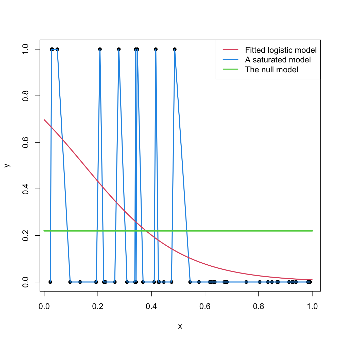
Figure 5.9: Fitted logistic regression versus a saturated model and the null model.
Formally, the deviance is defined through the difference of the log-likelihoods between the fitted model, \(\ell(\hat{\boldsymbol{\beta}}),\) and the saturated model, \(\ell_s.\) Computing \(\ell_s\) amounts to substitute \(\mu_i\) by \(Y_i\) in (5.20). If the canonical link function is used, this corresponds to setting \(\theta_i=g(Y_i)\) (recall (5.12)). The deviance is then defined as:
\[\begin{align*} D:=-2\left[\ell(\hat{\boldsymbol{\beta}})-\ell_s\right]\phi. \end{align*}\]
The log-likelihood \(\ell(\hat{\boldsymbol{\beta}})\) is always smaller than \(\ell_s\) (the saturated model is more likely given the sample, since it is the sample itself). As a consequence, the deviance is always greater than or equal to zero, being zero only if the fit of the model is perfect. It thus can be regarded as a distance between the fitted model and the saturated model.
If the canonical link function is employed, the deviance can be expressed as
\[\begin{align} D&=-\frac{2}{a(\phi)}\sum_{i=1}^n\left(Y_i\hat\theta_i-b(\hat\theta_i)-Y_ig(Y_i)+b(g(Y_i))\right)\phi\nonumber\\ &=\frac{2\phi}{a(\phi)}\sum_{i=1}^n\left(Y_i(g(Y_i)-\hat\theta_i)-b(g(Y_i))+b(\hat\theta_i)\right).\tag{5.30} \end{align}\]
In most of the cases, \(a(\phi)\propto\phi,\) so the deviance does not depend on \(\phi\). Expression (5.30) is interesting, since it delivers the following key insight:
The deviance generalizes the Residual Sum of Squares (RSS) of the linear model. The generalization is driven by the likelihood and its equivalence with the RSS in the linear model.
To see this insight, let’s consider the linear model in (5.30) by setting \(\phi=\sigma^2,\) \(a(\phi)=\phi,\) \(b(\theta)=\frac{\theta^2}{2},\) \(c(y,\phi)=-\frac{1}{2}\{\frac{y^2}{\phi}+\log(2\pi\phi)\},\) and \(\theta=\mu=\eta.\)181 Then:
\[\begin{align} D&=\frac{2\sigma^2}{\sigma^2}\sum_{i=1}^n\left(Y_i(Y_i-\hat{\eta}_i)-\frac{Y_i^2}{2}+\frac{\hat{\eta}_i^2}{2}\right)\nonumber\\ &=\sum_{i=1}^n\left(2Y_i^2-2Y_i\hat{\eta}_i-Y_i^2+\hat{\eta}_i^2\right)\nonumber\\ &=\sum_{i=1}^n\left(Y_i-\hat{\eta}_i\right)^2\nonumber\\ &=\mathrm{RSS}(\hat{\boldsymbol{\beta}}),\tag{5.31} \end{align}\]
since \(\hat{\eta}_i=\hat\beta_0+\hat\beta_1x_{i1}+\cdots+\hat\beta_px_{ip}.\) Remember that \(\mathrm{RSS}(\hat{\boldsymbol{\beta}})\) is just another name for the SSE.
A benchmark for evaluating the scale of the deviance is the null deviance,
\[\begin{align*} D_0:=-2\left[\ell(\hat{\beta}_0)-\ell_s\right]\phi, \end{align*}\]
which is the deviance of the model without predictors, the one featuring only an intercept, to the perfect model. In logistic regression, this model is
\[\begin{align*} Y \mid (X_1=x_1,\ldots,X_p=x_p)\sim \mathrm{Ber}(\mathrm{logistic}(\beta_0)) \end{align*}\]
and, in this case, \(\hat\beta_0=\mathrm{logit}(\frac{m}{n})=\log\left(\frac{\frac{m}{n}}{1-\frac{m}{n}}\right)\) where \(m\) is the number of \(1\)’s in \(Y_1,\ldots,Y_n\) (see Figure 5.9).
Using again (5.30), we can see that the null deviance is a generalization of the total sum of squares of the linear model (see Section 2.6):
\[\begin{align*} D_0=\sum_{i=1}^n\left(Y_i-\hat{\eta}_i\right)^2=\sum_{i=1}^n\left(Y_i-\hat\beta_0\right)^2=\mathrm{SST}, \end{align*}\]
since \(\hat\beta_0=\bar Y\) because there are no predictors.
The deviance and the null deviance offer a likelihood-based generalization of the ANOVA decomposition of SST into the RSS and the regression sum of squares. The difference between the null deviance and the deviance can be regarded as a generalization of the regression sum of squares. Figure 5.10 illustrates this deviance decomposition.

Figure 5.10: Pictorial representation of the model space indexed by the likelihood. The “size” of this space is given by the null deviance (\(D_0\)), while the deviance (\(D\)) measures the distance of the fitted model from the perfect model. This deviance decomposition is a likelihood-based generalization of the ANOVA decomposition.
Using the deviance and the null deviance, we can compare how much the model has improved by adding the predictors \(X_1,\ldots,X_p\) and quantify the percentage of deviance explained. This can be done by means of the \(R^2\) statistic, which is a generalization of the determination coefficient for linear regression:
\[\begin{align*} R^2:=1-\frac{D}{D_0}\stackrel{\substack{\mathrm{linear}\\ \mathrm{model}\\{}}}{=}1-\frac{\mathrm{SSE}}{\mathrm{SST}}. \end{align*}\]
The \(R^2\) for generalized linear models is a measure that shares the same philosophy with the determination coefficient in linear regression: it is a proportion of how good the model fit is. If perfect, \(D=0\) and \(R^2=1.\) If the predictors are not model-related with \(Y,\) then \(D=D_0\) and \(R^2=0.\)
However, this \(R^2\) has a different interpretation than in linear regression. In particular:
- Is not the percentage of variance explained by the model, but rather a ratio indicating how close is the fit to being perfect or the worst.
- It is not related to any correlation coefficient.
The deviance is returned by summary. It is important to recall that R refers to the deviance as the 'Residual deviance' and the null deviance is referred to as 'Null deviance'.
# Summary of model
nasa <- glm(fail.field ~ temp, family = "binomial", data = challenger)
summary_log <- summary(nasa)
summary_log
##
## Call:
## glm(formula = fail.field ~ temp, family = "binomial", data = challenger)
##
## Coefficients:
##             Estimate Std. Error z value Pr(>|z|)
## (Intercept)   7.5837     3.9146   1.937   0.0527 .
## temp         -0.4166     0.1940  -2.147   0.0318 *
## ---
## Signif. codes:  0 '***' 0.001 '**' 0.01 '*' 0.05 '.' 0.1 ' ' 1
##
## (Dispersion parameter for binomial family taken to be 1)
##
##     Null deviance: 28.267  on 22  degrees of freedom
## Residual deviance: 20.335  on 21  degrees of freedom
## AIC: 24.335
##
## Number of Fisher Scoring iterations: 5
# 'Residual deviance' is the deviance; 'Null deviance' is the null deviance

# Null model (only intercept)
null <- glm(fail.field ~ 1, family = "binomial", data = challenger)
summary_null <- summary(null)
summary_null
##
## Call:
## glm(formula = fail.field ~ 1, family = "binomial", data = challenger)
##
## Coefficients:
##             Estimate Std. Error z value Pr(>|z|)
## (Intercept)  -0.8267     0.4532  -1.824   0.0681 .
## ---
## Signif. codes:  0 '***' 0.001 '**' 0.01 '*' 0.05 '.' 0.1 ' ' 1
##
## (Dispersion parameter for binomial family taken to be 1)
##
##     Null deviance: 28.267  on 22  degrees of freedom
## Residual deviance: 28.267  on 22  degrees of freedom
## AIC: 30.267
##
## Number of Fisher Scoring iterations: 4

# Compute the R^2 with a function -- useful for repetitive computations
r2glm <- function(model) {

  summary_log <- summary(model)
  1 - summary_log$deviance / summary_log$null.deviance

}

# R^2
r2glm(nasa)
## [1] 0.280619
r2glm(null)
## [1] -6.661338e-16
A quantity related with the deviance is the scaled deviance:
\[\begin{align*} D^*:=\frac{D}{\phi}=-2\left[\ell(\hat{\boldsymbol{\beta}})-\ell_s\right]. \end{align*}\]
If \(\phi=1,\) such as in the binomial or Poisson regression models, then both the deviance and the scaled deviance agree. The scaled deviance has asymptotic distribution
\[\begin{align} D^*\stackrel{a}{\sim}\chi^2_{n-p-1},\tag{5.32} \end{align}\]
where \(\chi^2_{k}\) is the Chi-squared distribution with \(k\) degrees of freedom. In the case of the linear model, \(D^*=\frac{1}{\sigma^2}\mathrm{RSS}\) is exactly distributed as a \(\chi^2_{n-p-1}.\)
The result (5.32) provides a way of estimating \(\phi\) when it is unknown: match \(D^*\) with the expectation \(\mathbb{E}\left[\chi^2_{n-p-1}\right]=n-p-1.\) This provides
\[\begin{align*} \hat\phi_D:=\frac{-2(\ell(\hat{\boldsymbol{\beta}})-\ell_s)}{n-p-1}, \end{align*}\]
which, as expected, in the case of the linear model is equivalent to \(\hat\sigma^2\) as given in (2.15). More importantly, the scaled deviance can be used for performing hypotheses tests on sets of coefficients of a generalized linear model.
Assume we have one model, say \(M_2,\) with \(p_2\) predictors and another model, say \(M_1\), with \(p_1<p_2\) predictors that are contained in the set of predictors of the M2. In other words, assume \(M_1\) is nested within \(M_2.\) Then we can test the null hypothesis that the extra coefficients of \(M_2\) are simultaneously zero. For example, if \(M_1\) has the coefficients \(\{\beta_0,\beta_1,\ldots,\beta_{p_1}\}\) and M2 has coefficients \(\{\beta_0,\beta_1,\ldots,\beta_{p_1},\beta_{p_1+1},\ldots,\beta_{p_2}\},\) we can test
\[\begin{align*} H_0:\beta_{p_1+1}=\cdots=\beta_{p_2}=0\quad\text{vs.}\quad H_1:\beta_j\neq 0\text{ for any }p_1<j\leq p_2. \end{align*}\]
This can be done by means of the statistic182
\[\begin{align} D^*_{p_1}-D^*_{p_2}\stackrel{a,\,H_0}{\sim}\chi^2_{p_2-p_1}.\tag{5.33} \end{align}\]
If \(H_0\) is true,183 then \(D_{p_1}^*-D^*_{p_2}\) is expected to be small, thus we will reject \(H_0\) if the value of the statistic is above the \(\alpha\)-upper quantile of the \(\chi^2_{p_2-p_1}\), denoted as \(\chi^2_{\alpha;p_2-p_1}.\)
\(D^*\) apparently removes the effects of \(\phi,\) but it is still dependent on \(\phi,\) since this is hidden in the likelihood (see (5.30)). Therefore, \(D^*\) cannot be computed unless \(\phi\) is known, which forbids using (5.33). Hopefully, this dependence is removed by employing (5.32) and (5.33) and assuming that they are asymptotically independent. This gives the \(F\)-test for \(H_0\):
\[\begin{align*} F=\frac{(D^*_{p_1}-D^*_{p_2})/(p_2-p_1)}{D^*_{p_2}/(n-p_2-1)}=\frac{(D_{p_1}-D_{p_2})/(p_2-p_1)}{D_{p_2}/(n-p_2-1)}\stackrel{a,\,H_0}{\sim} F_{p_2-p_1,n-p_2-1}. \end{align*}\]
Note that \(F\) is perfectly computable, since \(\phi\) cancels due to the quotient (and because we assume that \(a(\phi)\propto\phi\)).
Note also that this is an extension of the \(F\)-test seen in Section 2.6: take \(p_1=0\) and \(p_2=p\) and then one tests the significance of all the predictors included in the model (both models contain intercept).
The computation of deviances and associated tests is done through anova, which implements the Analysis of Deviance. This is illustrated in the following code, which coincidentally also illustrates the inclusion of nonlinear transformations on the predictors.
# Polynomial predictors
nasa0 <- glm(fail.field ~ 1, family = "binomial", data = challenger)
nasa1 <- glm(fail.field ~ temp, family = "binomial", data = challenger)
nasa2 <- glm(fail.field ~ poly(temp, degree = 2), family = "binomial",
             data = challenger)
nasa3 <- glm(fail.field ~ poly(temp, degree = 3), family = "binomial",
             data = challenger)

# Plot fits
temp <- seq(-1, 35, l = 200)
tt <- data.frame(temp = temp)
plot(fail.field ~ temp, data = challenger, pch = 16, xlim = c(-1, 30),
     xlab = "Temperature", ylab = "Incident probability")
lines(temp, predict(nasa0, newdata = tt, type = "response"), col = 1)
lines(temp, predict(nasa1, newdata = tt, type = "response"), col = 2)
lines(temp, predict(nasa2, newdata = tt, type = "response"), col = 3)
lines(temp, predict(nasa3, newdata = tt, type = "response"), col = 4)
legend("bottomleft", legend = c("Null model", "Linear", "Quadratic", "Cubic"),
       lwd = 2, col = 1:4)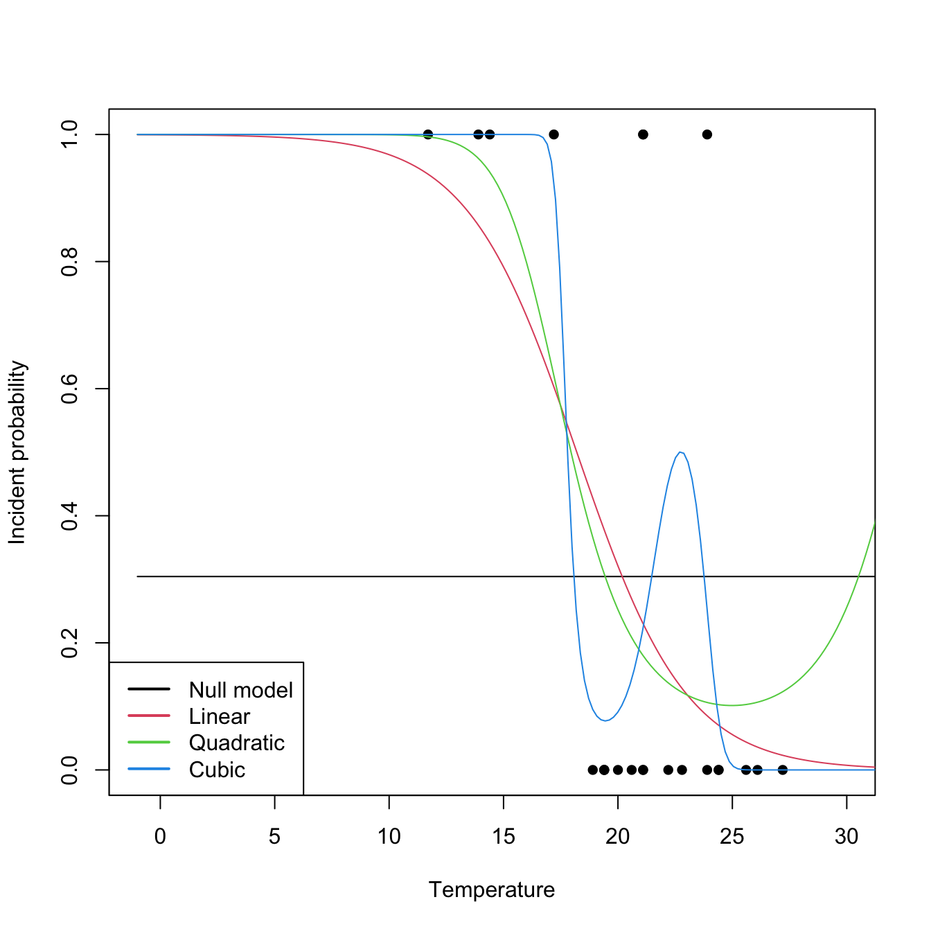
# R^2's
r2glm(nasa0)
## [1] -6.661338e-16
r2glm(nasa1)
## [1] 0.280619
r2glm(nasa2)
## [1] 0.3138925
r2glm(nasa3)
## [1] 0.4831863

# Chisq and F tests -- same results since phi is known
anova(nasa1, test = "Chisq")
## Analysis of Deviance Table
##
## Model: binomial, link: logit
##
## Response: fail.field
##
## Terms added sequentially (first to last)
##
##
##      Df Deviance Resid. Df Resid. Dev Pr(>Chi)
## NULL                    22     28.267
## temp  1   7.9323        21     20.335 0.004856 **
## ---
## Signif. codes:  0 '***' 0.001 '**' 0.01 '*' 0.05 '.' 0.1 ' ' 1
anova(nasa1, test = "F")
## Analysis of Deviance Table
##
## Model: binomial, link: logit
##
## Response: fail.field
##
## Terms added sequentially (first to last)
##
##
##      Df Deviance Resid. Df Resid. Dev      F   Pr(>F)
## NULL                    22     28.267
## temp  1   7.9323        21     20.335 7.9323 0.004856 **
## ---
## Signif. codes:  0 '***' 0.001 '**' 0.01 '*' 0.05 '.' 0.1 ' ' 1

# Incremental comparisons of nested models
anova(nasa1, nasa2, nasa3, test = "Chisq")
## Analysis of Deviance Table
##
## Model 1: fail.field ~ temp
## Model 2: fail.field ~ poly(temp, degree = 2)
## Model 3: fail.field ~ poly(temp, degree = 3)
##   Resid. Df Resid. Dev Df Deviance Pr(>Chi)
## 1        21     20.335
## 2        20     19.394  1   0.9405   0.3321
## 3        19     14.609  1   4.7855   0.0287 *
## ---
## Signif. codes:  0 '***' 0.001 '**' 0.01 '*' 0.05 '.' 0.1 ' ' 1
# Quadratic effects are not significant

# Cubic vs. linear
anova(nasa1, nasa3, test = "Chisq")
## Analysis of Deviance Table
##
## Model 1: fail.field ~ temp
## Model 2: fail.field ~ poly(temp, degree = 3)
##   Resid. Df Resid. Dev Df Deviance Pr(>Chi)
## 1        21     20.335
## 2        19     14.609  2    5.726   0.0571 .
## ---
## Signif. codes:  0 '***' 0.001 '**' 0.01 '*' 0.05 '.' 0.1 ' ' 1

# Example in Poisson regression
species1 <- glm(Species ~ ., data = species, family = poisson)
species2 <- glm(Species ~ Biomass * pH, data = species, family = poisson)

# Comparison
anova(species1, species2, test = "Chisq")
## Analysis of Deviance Table
##
## Model 1: Species ~ pH + Biomass
## Model 2: Species ~ Biomass * pH
##   Resid. Df Resid. Dev Df Deviance  Pr(>Chi)
## 1        86     99.242
## 2        84     83.201  2    16.04 0.0003288 ***
## ---
## Signif. codes:  0 '***' 0.001 '**' 0.01 '*' 0.05 '.' 0.1 ' ' 1
r2glm(species1)
## [1] 0.7806071
r2glm(species2)
## [1] 0.8160674
5.6 Model selection
The same discussion we did in Section 3.2 is applicable to generalized linear models with small changes:
- The deviance of the model (reciprocally the likelihood and the \(R^2\)) always decreases (increases) with the inclusion of more predictors – no matter whether they are significant or not.
- The excess of predictors in the model is paid by a larger variability in the estimation of the model which results in less precise prediction.
- Multicollinearity may hide significant variables, change the sign of them, and result in an increase of the variability of the estimation.
- Roughly speaking, the BIC is consistent in performing model-selection, and penalizes more the complex models when compared to AIC and LOOCV.
In addition, variable selection can also be done with the lasso for generalized linear models, as seen in Section 5.8.
Stepwise selection can be done through step as in linear models.184 Conveniently, summary also reports the AIC:
# Models
nasa1 <- glm(fail.field ~ temp, family = "binomial", data = challenger)
nasa2 <- glm(fail.field ~ temp + pres.field, family = "binomial",
             data = challenger)

# Summaries
summary(nasa1)
##
## Call:
## glm(formula = fail.field ~ temp, family = "binomial", data = challenger)
##
## Coefficients:
##             Estimate Std. Error z value Pr(>|z|)
## (Intercept)   7.5837     3.9146   1.937   0.0527 .
## temp         -0.4166     0.1940  -2.147   0.0318 *
## ---
## Signif. codes:  0 '***' 0.001 '**' 0.01 '*' 0.05 '.' 0.1 ' ' 1
##
## (Dispersion parameter for binomial family taken to be 1)
##
##     Null deviance: 28.267  on 22  degrees of freedom
## Residual deviance: 20.335  on 21  degrees of freedom
## AIC: 24.335
##
## Number of Fisher Scoring iterations: 5
summary(nasa2)
##
## Call:
## glm(formula = fail.field ~ temp + pres.field, family = "binomial",
##     data = challenger)
##
## Coefficients:
##              Estimate Std. Error z value Pr(>|z|)
## (Intercept)  6.642709   4.038547   1.645   0.1000
## temp        -0.435032   0.197008  -2.208   0.0272 *
## pres.field   0.009376   0.008821   1.063   0.2878
## ---
## Signif. codes:  0 '***' 0.001 '**' 0.01 '*' 0.05 '.' 0.1 ' ' 1
##
## (Dispersion parameter for binomial family taken to be 1)
##
##     Null deviance: 28.267  on 22  degrees of freedom
## Residual deviance: 19.078  on 20  degrees of freedom
## AIC: 25.078
##
## Number of Fisher Scoring iterations: 5

# AICs
AIC(nasa1) # Better
## [1] 24.33485
AIC(nasa2)
## [1] 25.07821
step works analogously as in linear regression. An illustration is given next for a predicting binary variable that measures whether a Boston suburb (Boston dataset from Section 3.1) is wealthy or not. The binary variable is medv > 25: it is TRUE (1) for suburbs with median house value larger than 25000$ and FALSE (0) otherwise.185 The cutoff 25000$ corresponds to the 25% richest suburbs.
# Boston dataset
data(Boston, package = "MASS")

# Model whether a suburb has a median house value larger than $25000
mod <- glm(I(medv > 25) ~ ., data = Boston, family = "binomial")
summary(mod)
##
## Call:
## glm(formula = I(medv > 25) ~ ., family = "binomial", data = Boston)
##
## Coefficients:
##              Estimate Std. Error z value Pr(>|z|)
## (Intercept)  5.312511   4.876070   1.090 0.275930
## crim        -0.011101   0.045322  -0.245 0.806503
## zn           0.010917   0.010834   1.008 0.313626
## indus       -0.110452   0.058740  -1.880 0.060060 .
## chas         0.966337   0.808960   1.195 0.232266
## nox         -6.844521   4.483514  -1.527 0.126861
## rm           1.886872   0.452692   4.168 3.07e-05 ***
## age          0.003491   0.011133   0.314 0.753853
## dis         -0.589016   0.164013  -3.591 0.000329 ***
## rad          0.318042   0.082623   3.849 0.000118 ***
## tax         -0.010826   0.004036  -2.682 0.007314 **
## ptratio     -0.353017   0.122259  -2.887 0.003884 **
## black       -0.002264   0.003826  -0.592 0.554105
## lstat       -0.367355   0.073020  -5.031 4.88e-07 ***
## ---
## Signif. codes:  0 '***' 0.001 '**' 0.01 '*' 0.05 '.' 0.1 ' ' 1
##
## (Dispersion parameter for binomial family taken to be 1)
##
##     Null deviance: 563.52  on 505  degrees of freedom
## Residual deviance: 209.11  on 492  degrees of freedom
## AIC: 237.11
##
## Number of Fisher Scoring iterations: 7
r2glm(mod)
## [1] 0.628923

# With BIC -- ends up with only the significant variables and a similar R^2
mod_bic <- step(mod, trace = 0, k = log(nrow(Boston)))
summary(mod_bic)
##
## Call:
## glm(formula = I(medv > 25) ~ indus + rm + dis + rad + tax + ptratio +
##     lstat, family = "binomial", data = Boston)
##
## Coefficients:
##              Estimate Std. Error z value Pr(>|z|)
## (Intercept)  1.556433   3.948818   0.394 0.693469
## indus       -0.143236   0.054771  -2.615 0.008918 **
## rm           1.950496   0.441794   4.415 1.01e-05 ***
## dis         -0.426830   0.111572  -3.826 0.000130 ***
## rad          0.301060   0.076542   3.933 8.38e-05 ***
## tax         -0.010240   0.003631  -2.820 0.004800 **
## ptratio     -0.404964   0.112086  -3.613 0.000303 ***
## lstat       -0.384823   0.069121  -5.567 2.59e-08 ***
## ---
## Signif. codes:  0 '***' 0.001 '**' 0.01 '*' 0.05 '.' 0.1 ' ' 1
##
## (Dispersion parameter for binomial family taken to be 1)
##
##     Null deviance: 563.52  on 505  degrees of freedom
## Residual deviance: 215.03  on 498  degrees of freedom
## AIC: 231.03
##
## Number of Fisher Scoring iterations: 7
r2glm(mod_bic)
## [1] 0.6184273
The logistic model is at the intersection between regression models and classification methods. Therefore, the search for adequate predictors to be included in the model can also be done in terms of the classification performance. Although we do not explore in detail this direction, we simply mention how the overall predictive accuracy can be summarized with the confusion matrix (also called hit matrix):
| Reality vs. classified | \(\hat Y=0\) | \(\hat Y=1\) |
|---|---|---|
| \(Y=0\) | True Negative (TN) | False Positive (FP) |
| \(Y=1\) | False Negative (FN) | True Positive (TP) |
The accuracy, \(\frac{\text{TN}+\text{TP}}{n},\) is the percentage of correct classifications. Beyond accuracy, the confusion matrix entries give rise to other performance metrics: sensitivity (or recall), \(\frac{\text{TP}}{\text{TP}+\text{FN}}\); specificity, \(\frac{\text{TN}}{\text{TN}+\text{FP}}\); and precision, \(\frac{\text{TP}}{\text{TP}+\text{FP}}\). These are particularly informative when classes are imbalanced, since accuracy can be misleadingly high by simply predicting the majority class. The F1 score, \(\frac{2\cdot\text{precision}\cdot\text{recall}}{\text{precision}+\text{recall}}=\frac{2\,\text{TP}}{2\,\text{TP}+\text{FP}+\text{FN}}\), is the harmonic mean of precision and recall and provides a single balanced measure when both false positives and false negatives matter.
The confusion matrix is easily computed with the table function which, whenever called with two vectors, computes the cross-table between those two vectors.
# Fitted probabilities for Y = 1
nasa$fitted.values
##          1          2          3          4          5          6          7          8          9         10
## 0.42778935 0.23014393 0.26910358 0.32099837 0.37772880 0.15898364 0.12833090 0.23014393 0.85721594 0.60286639
##         11         12         13         14         15         16         17         18         19         20
## 0.23014393 0.04383877 0.37772880 0.93755439 0.37772880 0.08516844 0.23014393 0.02299887 0.07027765 0.03589053
##         21         22         23
## 0.08516844 0.07027765 0.82977495

# Classified Y's
y_hat <- nasa$fitted.values > 0.5

# Confusion matrix:
# - 16 correctly classified as 0
# - 4 correctly classified as 1
# - 3 incorrectly classified as 0
tab <- table(challenger$fail.field, y_hat)
tab
##    y_hat
##     FALSE TRUE
##   0    16    0
##   1     3    4

# Accuracy (ratio of correct classifications)
sum(diag(tab)) / sum(tab)
## [1] 0.8695652
Note that the classification rule \(\hat{Y}=1_{\{\mathrm{logistic}(\hat{\eta}(\mathbf{x}))>0.5\}}\) uses \(0.5\) as the default threshold, but this choice is arbitrary. Different thresholds yield different confusion matrices, trading off sensitivity against specificity. The full tradeoff as the threshold varies is captured by the ROC curve (Receiver Operating Characteristic), but we do not pursue that here.
It is important to recall that the confusion matrix will be always biased towards unrealistically good classification rates if it is computed in the same sample used for fitting the logistic model. An approach based on data-splitting/cross-validation is therefore needed to estimate unbiasedly the confusion matrix.
Exercise 5.7 For the Boston dataset, do the following:
- Compute the confusion matrix and accuracy for the regression
I(medv > 25) ~ .. - Fit
I(medv > 25) ~ .but now using only the first 300 observations ofBoston, the training dataset. - For the previous model, predict the probability of the responses and classify them into
0or1in the last \(206\) observations, the testing dataset. - Compute the confusion matrix and accuracy for the new predictions. Check that the accuracy is smaller than the one in the first point.
5.7 Model diagnostics
As it was implicit in Section 5.2, generalized linear models are built on some probabilistic assumptions that are required for performing inference on the model parameters \(\boldsymbol{\beta}\) and \(\phi.\)
In general, if we employ the canonical link function, we assume that the data has been generated from (independence is implicit)
\[\begin{align} Y&\mid (X_1=x_{1},\ldots,X_p=x_{p})\sim\mathrm{E}(\eta(x_1,\ldots,x_p),\phi,a,b,c),\tag{5.34} \end{align}\]
in such a way that
\[\begin{align*} \mu=\mathbb{E}[Y \mid X_1=x_{1},\ldots,X_p=x_{p}]=g^{-1}(\eta), \end{align*}\]
and \(\eta(x_1,\ldots,x_p)=\beta_0+\beta_1x_{1}+\cdots+\beta_px_{p}.\)
In the case of the logistic and Poisson regressions, both with canonical link functions, the general model takes the form (independence is implicit)
\[\begin{align} Y \mid (X_1=x_1,\ldots,X_p=x_p)&\sim\mathrm{Ber}\left(\mathrm{logistic}(\eta)\right), \tag{5.35}\\ Y \mid (X_1=x_1,\ldots,X_p=x_p)&\sim\mathrm{Pois}\left(e^{\eta}\right). \tag{5.36} \end{align}\]
The assumptions behind (5.34), (5.35), and (5.36) are:
- Linearity in the transformed expectation: \(\mathbb{E}[Y \mid X_1=x_1,\ldots,X_p=x_p]=g^{-1}\left(\beta_0+\beta_1x_1+\cdots+\beta_px_p\right).\)
- Response distribution: \(Y \mid \mathbf{X}=\mathbf{x}\sim\mathrm{E}(\eta(\mathbf{x}),\phi,a,b,c)\) (the scale \(\phi\) and the functions \(a,b,c\) are constant for \(\mathbf{x}\)).
- Independence: \(Y_1,\ldots,Y_n\) are independent, conditionally on \(\mathbf{X}_1,\ldots,\mathbf{X}_n.\)
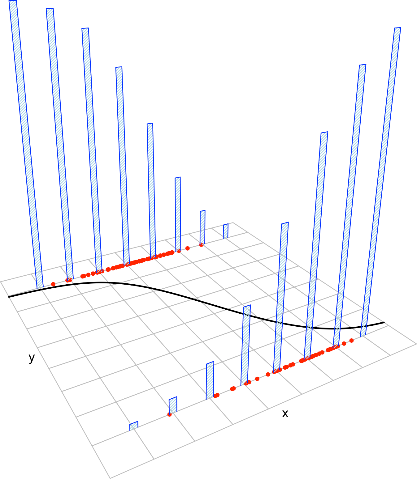
Figure 5.11: The key concepts of the logistic model. The red points represent a sample with population logistic curve \(y=\mathrm{logistic}(\beta_0+\beta_1x),\) shown in black. The blue bars represent the conditional probability mass functions of \(Y\) given \(X=x,\) whose means lie in the logistic curve.
There are two important points of the linear model assumptions “missing” here:
- Where is homoscedasticity? Homoscedasticity is specific to certain exponential family distributions in which \(\theta\) does not affect the variance. This is not the case for binomial or Poisson distributions variables, which result in heteroscedastic models. Also, homoscedasticity is the consequence of assumption ii in the case of the normal distribution.
- Where are the errors? The errors are not fundamental for building the linear model, but just a helpful concept related to least squares. The linear model can be constructed “without errors” directly using (2.8).
Recall that:
- Nothing is said about the distribution of \(X_1,\ldots,X_p.\) They could be deterministic or random. They could be discrete or continuous.
- \(X_1,\ldots,X_p\) are not required to be independent between them.
Checking the assumptions of a generalized linear model is more complicated than what we did in Section 3.5. The reason is the heterogeneity and heteroscedasticity of the responses, which makes the inspection of the residuals \(Y_i-\hat Y_i\) complicated.186 The first step is to construct some residuals \(\hat\varepsilon_i\) that are simpler to analyze.
The deviance residuals are the generalization of the residuals \(\hat\varepsilon_i=Y_i-\hat Y_i\) from the linear model. They are constructed using the analogy between the deviance and the RSS seen in (5.31). The deviance can be expressed into a sum of terms associated with each datum (recall, e.g., (5.30)):
\[\begin{align*} D=\sum_{i=1}^n d_i. \end{align*}\]
For the linear model, \(d_i=\hat\varepsilon_i^2,\) since \(D=\mathrm{RSS}(\hat{\boldsymbol{\beta}}).\) Based on this, we can define the deviance residuals as
\[\begin{align*} \hat\varepsilon_i^D:=\mathrm{sign}(Y_i-\hat \mu_i)\sqrt{d_i},\quad i=1,\ldots,n \end{align*}\]
and have a generalization of \(\hat\varepsilon_i\) for generalized linear models. This definition has interesting distributional consequences. From (5.32), we know that \(D^*\stackrel{a}{\sim}\chi_{n-p-1}^2.\) This suggests187 that
\[\begin{align} \hat\varepsilon_i^D\text{ are approximately normal if the model holds}.\tag{5.37} \end{align}\]
The previous statement is of variable accuracy, depending on the model, sample size, and distribution of the predictors.188 In the linear model, it is exact and \((\hat\varepsilon_1^D,\ldots,\hat\varepsilon_n^D)\) are distributed exactly as a \(\mathcal{N}_n(\mathbf{0},\sigma^2(\mathbf{I}-\mathbf{H})),\) where \(\mathbf{H}=\mathbb{X}(\mathbb{X}^\top\mathbb{X})^{-1}\mathbb{X}^\top.\)
The deviance residuals are key for the diagnostics of generalized linear models. Whenever we refer to “residuals”, we understand that we refer to the deviance residuals (since several definitions of residuals are possible). They are also the residuals returned in R, either by glm$residuals or by residuals(glm).
The definition of the deviance residuals has interesting connections:
- If the canonical function is employed, then \(\sum_{i=1}^n \hat\varepsilon_i^D=0,\) as in the linear model.
- The estimate of the scale parameter can be seen as \(\hat\phi_D=\frac{\sum_{i=1}^n(\hat\varepsilon_i^D)^2}{n-p-1},\) which is perfectly coherent with \(\hat\sigma^2\) in the linear model.
- Therefore, \(\hat\phi_D\) is the sample variance of \(\hat\varepsilon_1^D,\ldots,\hat\varepsilon_n^D,\) which suggests that \(\phi\) is the asymptotic variance of the population deviance residuals, in other words, \(\mathbb{V}\mathrm{ar}[\varepsilon^D]\approx \phi.\)
- The deviance residuals equal the standard residuals in the linear model.
The script used for generating the following (perhaps surprising) Figures 5.12–5.23 is available here.
5.7.1 Linearity
Linearity between the transformed expectation of \(Y\) and the predictors \(X_1,\ldots,X_p\) is the building block of generalized linear models. If this assumption fails, then all the conclusions we might extract from the analysis are suspected to be flawed. Therefore it is a key assumption.
5.7.1.1 How to check it
We use the residuals vs. fitted values plot, which for generalized linear models is the scatterplot of \(\{(\hat{\eta}_i, \hat{\varepsilon}_i^D)\}_{i=1}^n.\) Recall that it is not the scatterplot of \(\{(\hat{Y}_i, \hat{\varepsilon}_i)\}_{i=1}^n.\) Under linearity, we expect that there is no trend in the residuals \(\hat\varepsilon_i^D\) with respect to \(\hat \eta_i,\) in addition to the patterns inherent to the nature of the response. If nonlinearities are observed, it is worth plotting the regression terms of the model via termplot.
5.7.1.2 What to do it fails
Using an adequate nonlinear transformation for the problematic predictors or adding interaction terms might be helpful. Alternatively, considering a nonlinear transformation \(f\) for the response \(Y\) might also be helpful, at expenses of the same comments given in Section 3.5.1.
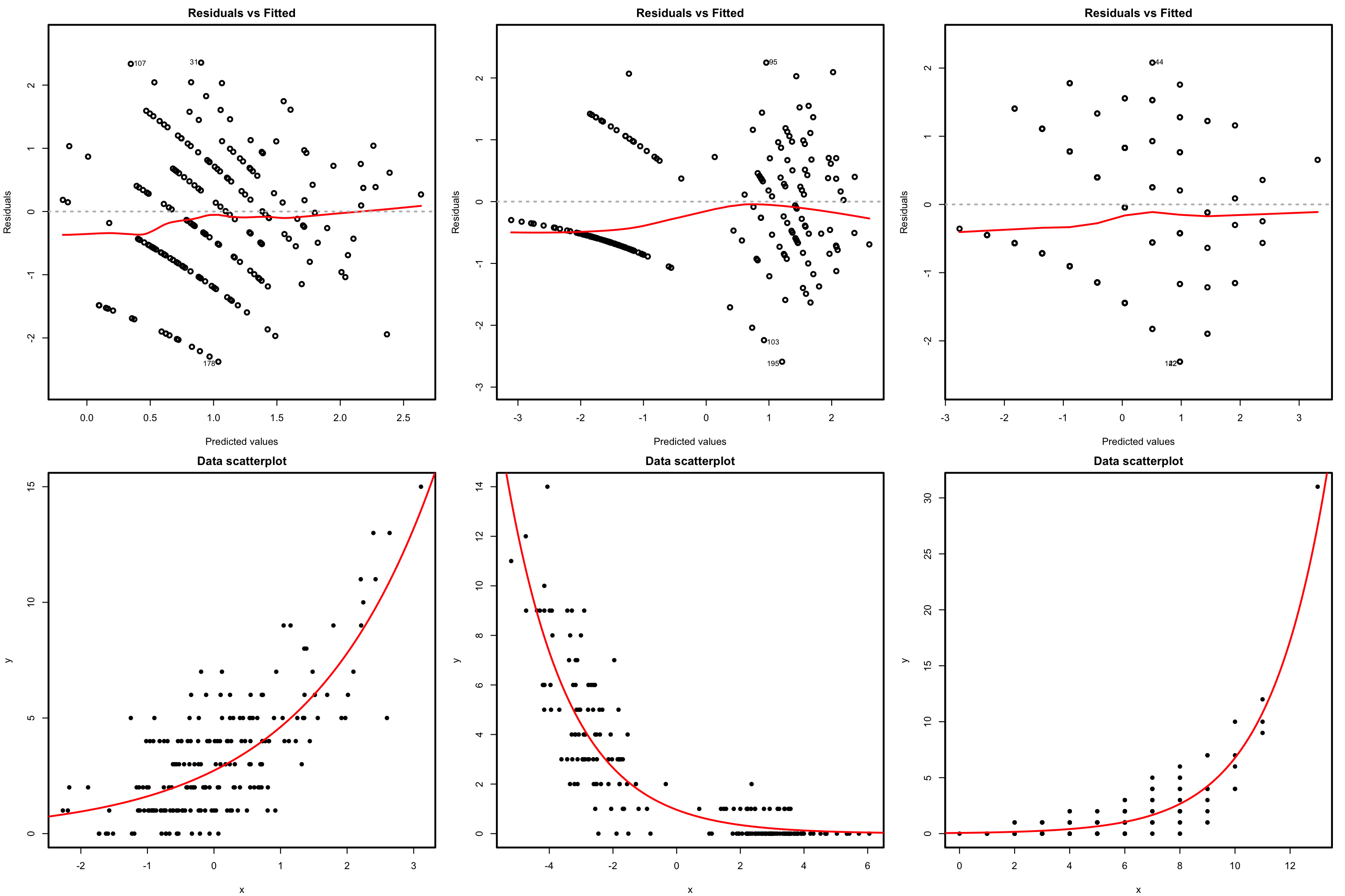
Figure 5.12: Residuals vs. fitted values plots (first row) for datasets (second row) respecting the linearity assumption in Poisson regression.
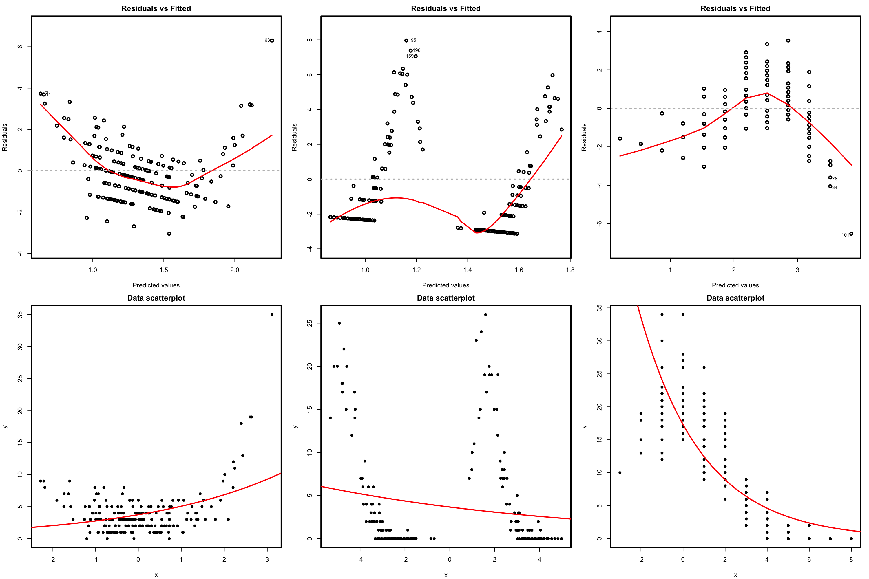
Figure 5.13: Residuals vs. fitted values plots (first row) for datasets (second row) violating the linearity assumption in Poisson regression.
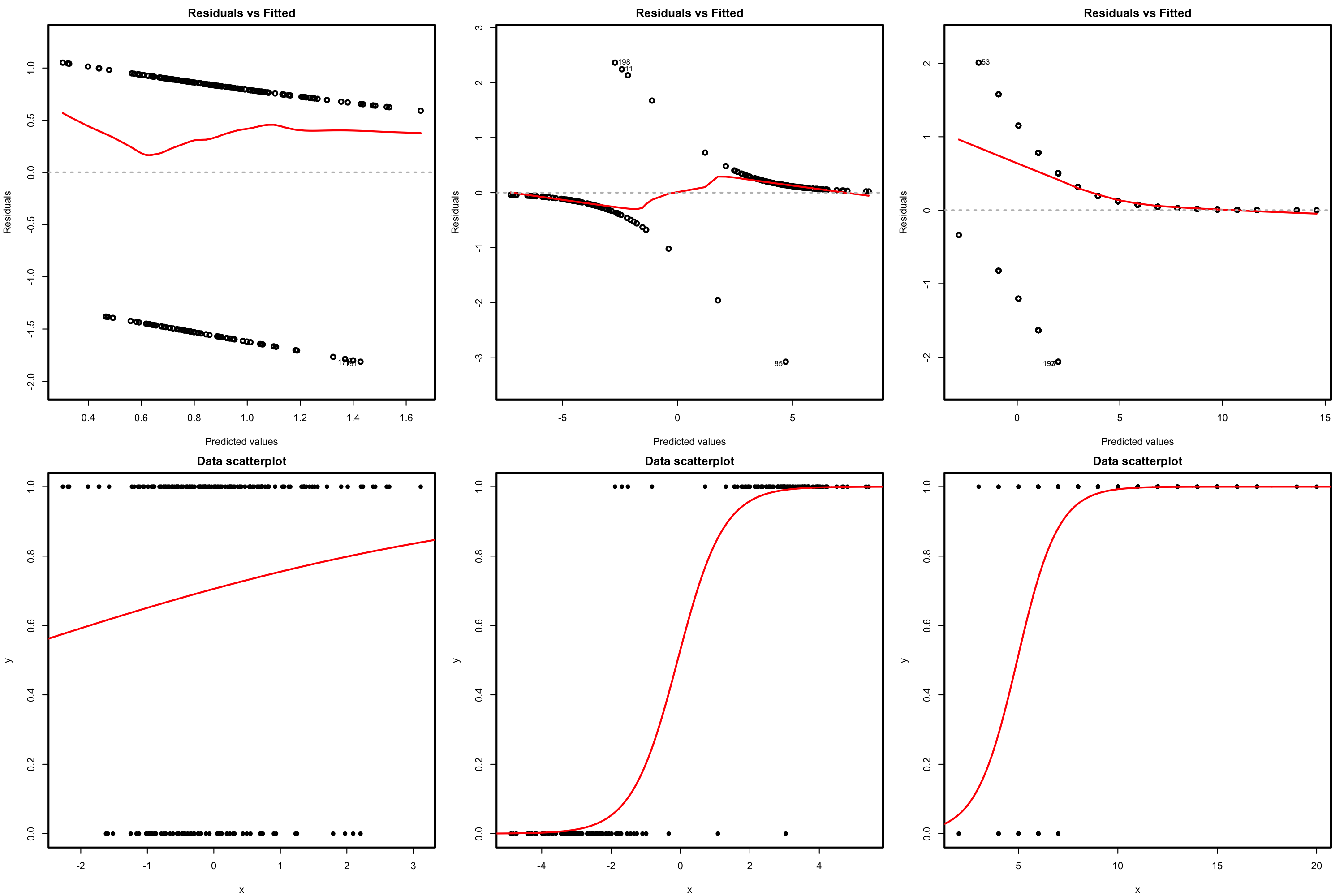
Figure 5.14: Residuals vs. fitted values plots (first row) for datasets (second row) respecting the linearity assumption in logistic regression.
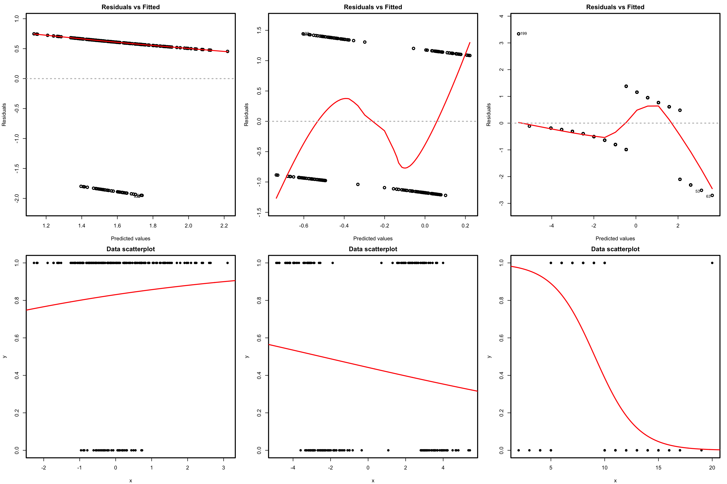
Figure 5.15: Residuals vs. fitted values plots (first row) for datasets (second row) violating the linearity assumption in logistic regression.
5.7.2 Response distribution
The approximate normality in the deviance residuals allows us to evaluate how well satisfied the assumption of the response distribution is. The good news is that we can do so without relying on ad-hoc tools for each distribution.189 The bad news is that we have to pay an important price in terms of inexactness, since we employ an asymptotic distribution. The speed of this asymptotic convergence and the effective validity of (5.37) largely depends on several aspects: distribution of the response, sample size, and distribution of the predictors.
5.7.2.1 How to check it
The QQ-plot allows us to check if the standardized residuals follow a \(\mathcal{N}(0,1).\) Under the correct distribution of the response, we expect the points to align with the diagonal line. It is usual to have departures from the diagonal in the extremes other than in the center, even under normality, although these departures are more evident if the data is non-normal. Unfortunately, it is also possible to have severe departures from normality even if the model is perfectly correct, see below. The reason is simply that the deviance residuals are significantly non-normal, which happens often in logistic regression.
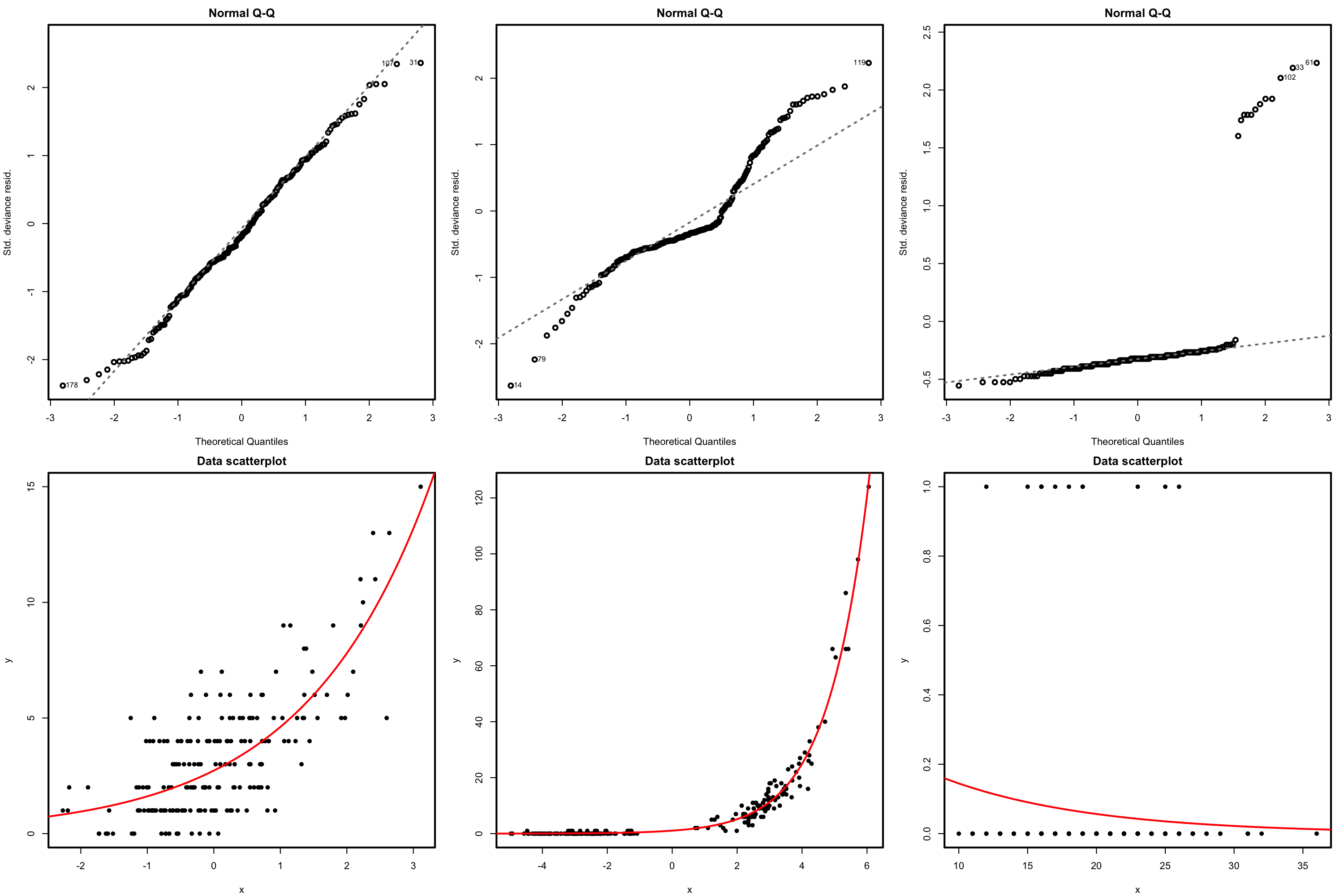
Figure 5.16: QQ-plots for the deviance residuals (first row) for datasets (second row) respecting the response distribution assumption for Poisson regression.
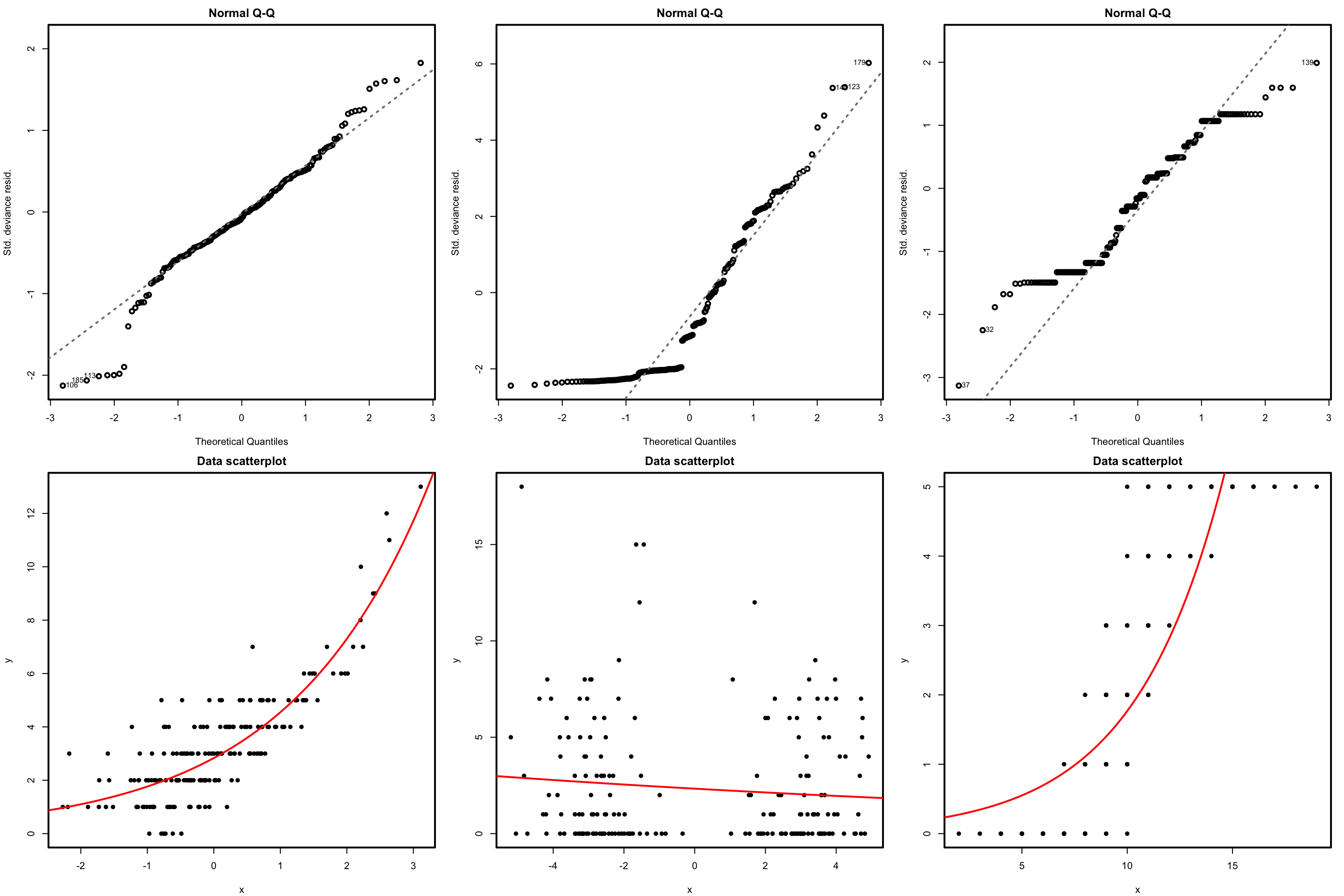
Figure 5.17: QQ-plots for the deviance residuals (first row) for datasets (second row) violating the response distribution assumption for Poisson regression.
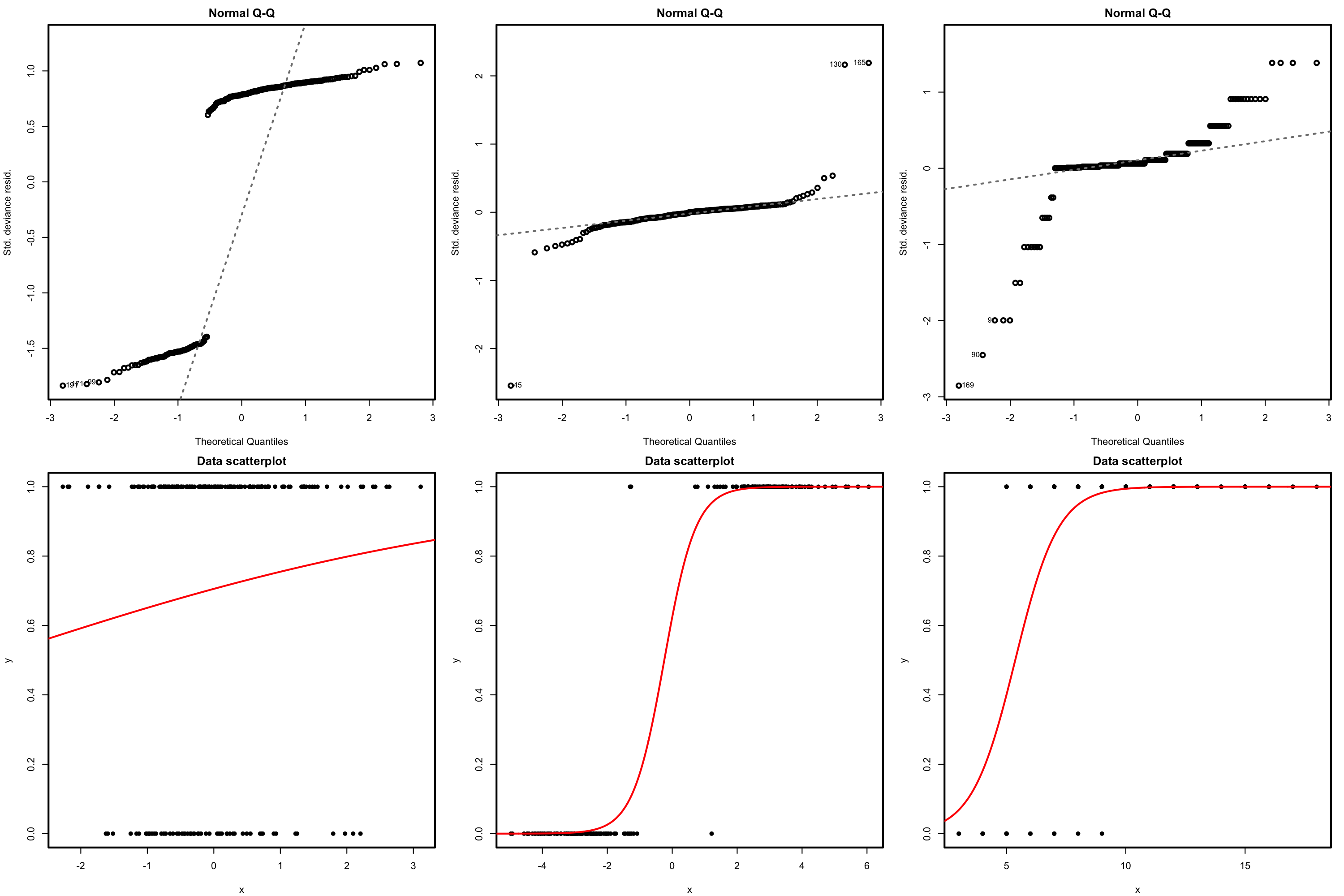
Figure 5.18: QQ-plots for the deviance residuals (first row) for datasets (second row) respecting the response distribution assumption for logistic regression.
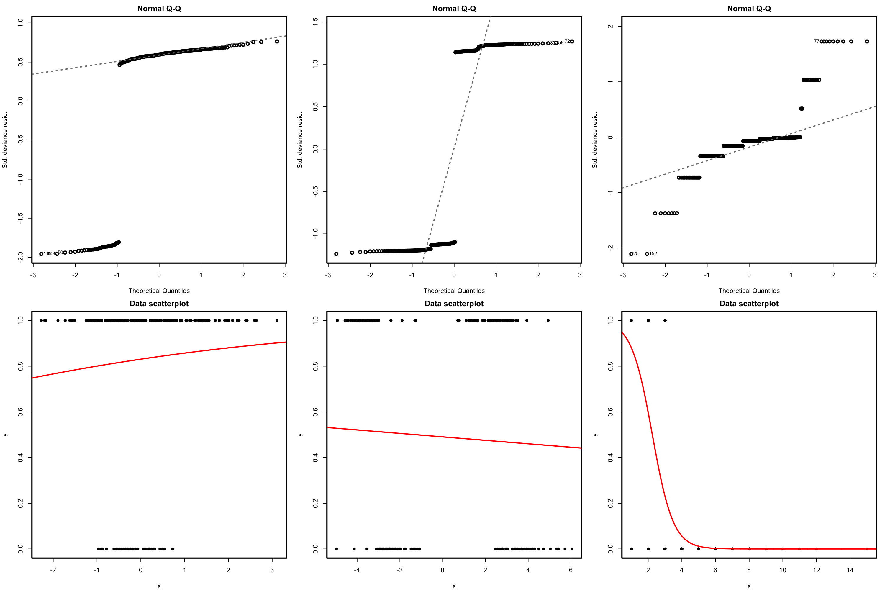
Figure 5.19: QQ-plots for the deviance residuals (first row) for datasets (second row) violating the response distribution assumption for logistic regression.
5.7.2.2 What to do if it fails
Patching the distribution assumption is not easy and requires the consideration of more flexible models. One possibility is to transform \(Y\) by means of one of the transformations discussed in Section 3.5.2, of course at the price of modeling the transformed response rather than \(Y.\)
5.7.3 Independence
Independence is also a key assumption: it guarantees that the amount of information that we have on the relationship between \(Y\) and \(X_1,\ldots,X_p\) with \(n\) observations is maximal.
5.7.3.1 How to check it
The presence of autocorrelation in the residuals can be examined by means of a serial plot of the residuals. Under uncorrelation, we expect the series to show no tracking of the residuals, which is a sign of positive serial correlation. Negative serial correlation can be identified in the form of a small-large or positive-negative systematic alternation of the residuals. This can be explored better with lag.plot, as seen in Section 3.5.4.
5.7.3.2 What to do if it fails
As in the linear model, little can be done if there is dependence in the data, once this has been collected. If serial dependence is present, a differentiation of the response may lead to independent observations.
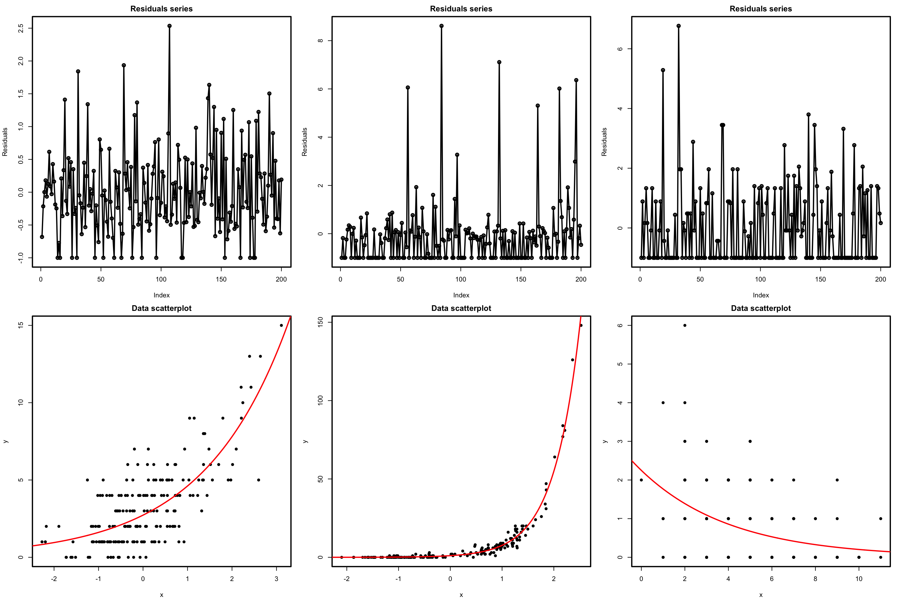
Figure 5.20: Serial plots of the residuals (first row) for datasets (second row) respecting the independence assumption for Poisson regression.
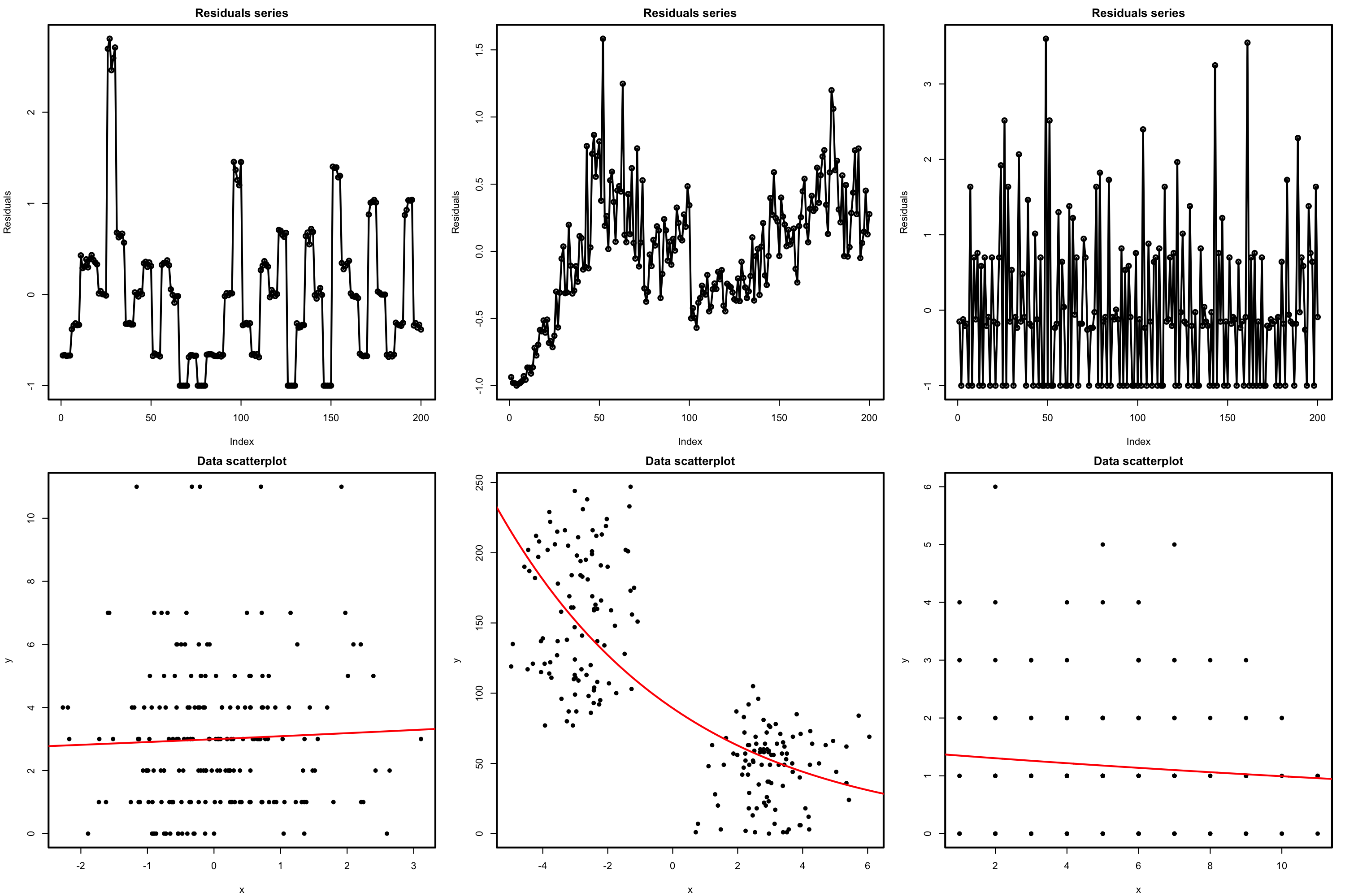
Figure 5.21: Serial plots of the residuals (first row) for datasets (second row) violating the independence assumption for Poisson regression.
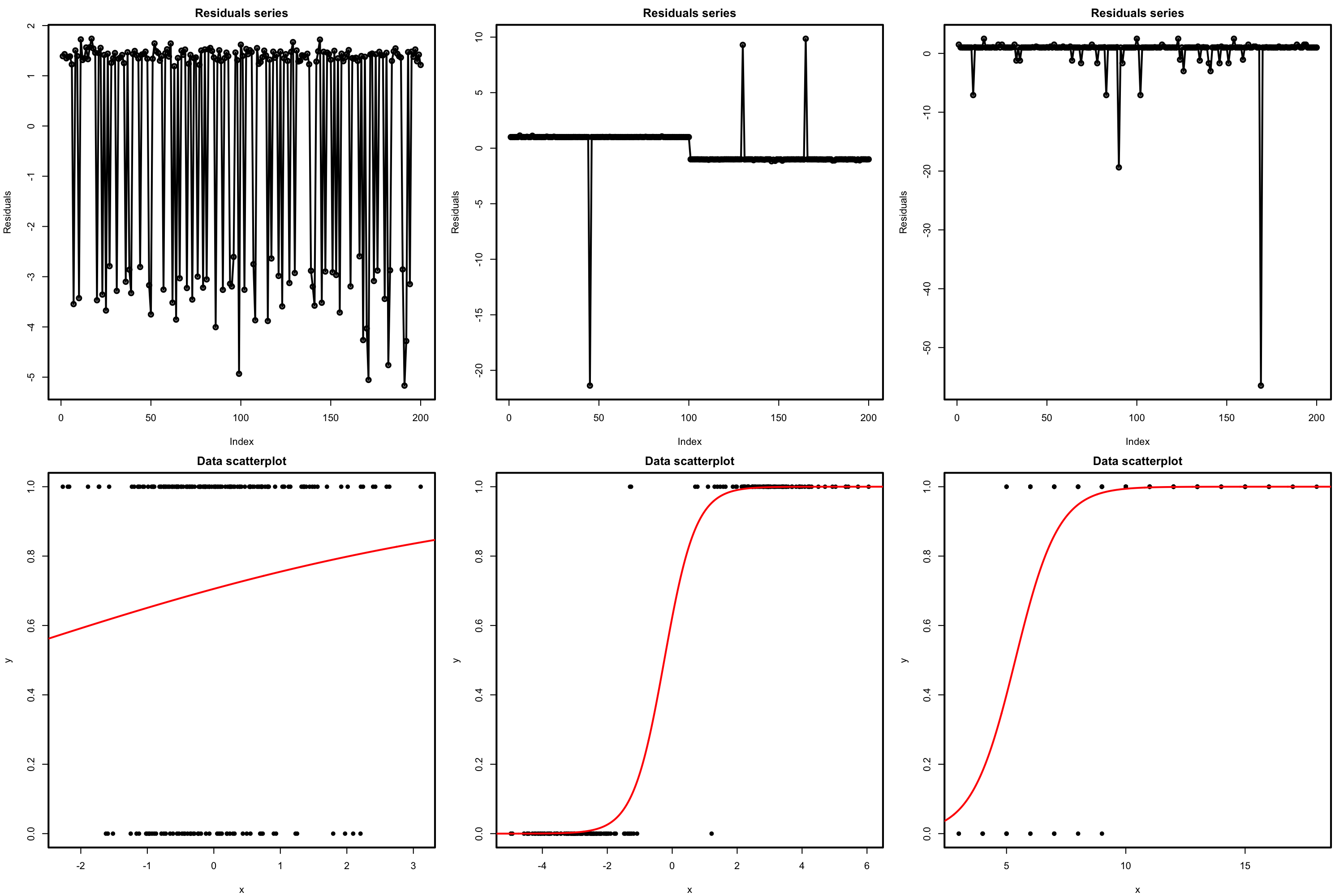
Figure 5.22: Serial plots of the residuals (first row) for datasets (second row) respecting the independence assumption for logistic regression.
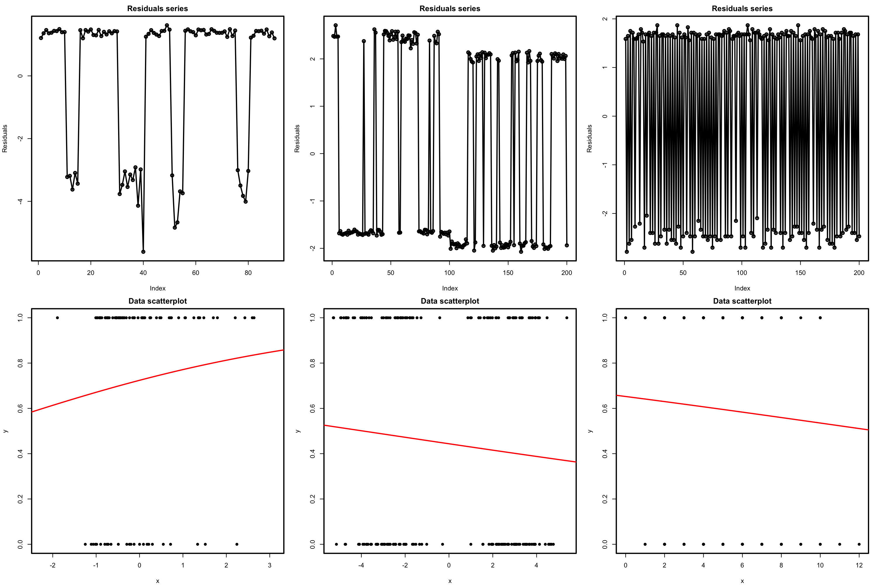
Figure 5.23: Serial plots of the residuals (first row) for datasets (second row) violating the independence assumption for logistic regression.
5.7.4 Multicollinearity
Multicollinearity can also be present in generalized linear models. Despite the nonlinear effect of the predictors on the response, the predictors are combined linearly in (5.4). Due to this, if two or more predictors are highly correlated between them, the fit of the model will be compromised since the individual linear effect of each predictor will be hard to separate from the rest of correlated predictors.
Then, a useful way of detecting multicollinearity is to inspect the VIF of each coefficient. The situation is exactly the same as in linear regression, since VIF looks only into the linear relations of the predictors. Therefore, the rule of thumb is the same as in Section 3.5.5:
- VIF close to 1: absence of multicollinearity.
- VIF larger than 5 or 10: problematic amount of multicollinearity. Advised to remove the predictor with largest VIF.
# Create predictors with multicollinearity: x4 depends on the rest
set.seed(45678)
x1 <- rnorm(100)
x2 <- 0.5 * x1 + rnorm(100)
x3 <- 0.5 * x2 + rnorm(100)
x4 <- -x1 + x2 + rnorm(100, sd = 0.25)

# Response
z <- 1 + 0.5 * x1 + 2 * x2 - 3 * x3 - x4
y <- rbinom(n = 100, size = 1, prob = 1/(1 + exp(-z)))
data <- data.frame(x1 = x1, x2 = x2, x3 = x3, x4 = x4, y = y)

# Correlations -- none seems suspicious
cor(data)
##            x1         x2         x3         x4           y
## x1  1.0000000 0.38254782  0.2142011 -0.5261464  0.20198825
## x2  0.3825478 1.00000000  0.5167341  0.5673174  0.07456324
## x3  0.2142011 0.51673408  1.0000000  0.2500123 -0.49853746
## x4 -0.5261464 0.56731738  0.2500123  1.0000000 -0.11188657
## y   0.2019882 0.07456324 -0.4985375 -0.1118866  1.00000000

# Abnormal generalized variance inflation factors: largest for x4, we remove it
mod_multico <- glm(y ~ x1 + x2 + x3 + x4, family = "binomial")
car::vif(mod_multico)
##       x1       x2       x3       x4
## 27.84756 36.66514  4.94499 36.78817

# Without x4
mod_clean <- glm(y ~ x1 + x2 + x3, family = "binomial")

# Generalized variance inflation factors normal
car::vif(mod_clean)
##       x1       x2       x3
## 1.674300 2.724351 3.743940

# Comparison
summary(mod_multico)
##
## Call:
## glm(formula = y ~ x1 + x2 + x3 + x4, family = "binomial")
##
## Coefficients:
##             Estimate Std. Error z value Pr(>|z|)
## (Intercept)   1.2527     0.4008   3.125  0.00178 **
## x1           -3.4269     1.8225  -1.880  0.06007 .
## x2            6.9627     2.1937   3.174  0.00150 **
## x3           -4.3688     0.9312  -4.691 2.71e-06 ***
## x4           -5.0047     1.9440  -2.574  0.01004 *
## ---
## Signif. codes:  0 '***' 0.001 '**' 0.01 '*' 0.05 '.' 0.1 ' ' 1
##
## (Dispersion parameter for binomial family taken to be 1)
##
##     Null deviance: 132.81  on 99  degrees of freedom
## Residual deviance:  59.76  on 95  degrees of freedom
## AIC: 69.76
##
## Number of Fisher Scoring iterations: 7
summary(mod_clean)
##
## Call:
## glm(formula = y ~ x1 + x2 + x3, family = "binomial")
##
## Coefficients:
##             Estimate Std. Error z value Pr(>|z|)
## (Intercept)   0.9237     0.3221   2.868 0.004133 **
## x1            1.2803     0.4235   3.023 0.002502 **
## x2            1.7946     0.5290   3.392 0.000693 ***
## x3           -3.4838     0.7491  -4.651 3.31e-06 ***
## ---
## Signif. codes:  0 '***' 0.001 '**' 0.01 '*' 0.05 '.' 0.1 ' ' 1
##
## (Dispersion parameter for binomial family taken to be 1)
##
##     Null deviance: 132.813  on 99  degrees of freedom
## Residual deviance:  68.028  on 96  degrees of freedom
## AIC: 76.028
##
## Number of Fisher Scoring iterations: 65.8 Shrinkage
Enforcing sparsity in generalized linear models can be done as how it was done in linear models. Ridge regression and lasso can be generalized with glmnet with little differences in practice.
What we want is to bias the estimates of \(\boldsymbol{\beta}\) towards being non-null only in the most important relations between the response and predictors. To achieve that, we add a penalization term to the maximum likelihood estimation of \(\boldsymbol{\beta}\):190
\[\begin{align} -\ell(\boldsymbol{\beta})+\lambda\sum_{j=1}^p (\alpha|\beta_j|+(1-\alpha)|\beta_j|^2).\tag{5.38} \end{align}\]
As in Section 4.1, ridge regression corresponds to \(\alpha=0\) (quadratic penalty) and lasso to \(\alpha=1\) (absolute value penalty). Obviously, if \(\lambda=0,\) we are back to the generalized linear models theory. The optimization of (5.38) gives
\[\begin{align} \hat{\boldsymbol{\beta}}_{\lambda,\alpha}:=\arg\min_{\boldsymbol{\beta}\in\mathbb{R}^{p+1}}\left\{ -\ell(\boldsymbol{\beta})+\lambda\sum_{j=1}^p (\alpha|\beta_j|+(1-\alpha)|\beta_j|^2)\right\}.\tag{5.39} \end{align}\]
Note that the sparsity is enforced in the slopes, not in the intercept, and that the link function \(g\) is not affecting the penalization term. As in linear models, the predictors need to be standardized if they have a different nature.
We illustrate the shrinkage in generalized linear models with the ISLR::Hitters dataset, where now the objective will be to predict NewLeague, a factor with levels A (standing for American League) and N (standing for National League). The variable indicates the player’s league at the end of 1986. The predictors employed are his statistics during 1986, and the objective is to see whether there is some distinctive pattern between the players in both leagues.
# Load data
data(Hitters, package = "ISLR")

# Include only predictors related with 1986 season and discard NA's
Hitters <- subset(Hitters, select = c(League, AtBat, Hits, HmRun, Runs, RBI,
                                      Walks, Division, PutOuts, Assists,
                                      Errors))
Hitters <- na.omit(Hitters)

# Response and predictors
y <- Hitters$League
x <- model.matrix(League ~ ., data = Hitters)[, -1]
After preparing the data, we perform the regressions.
# Ridge and lasso regressions
library(glmnet)
ridge_mod <- glmnet(x = x, y = y, alpha = 0, family = "binomial")
lasso_mod <- glmnet(x = x, y = y, alpha = 1, family = "binomial")

# Solution paths versus lambda
plot(ridge_mod, label = TRUE, xvar = "lambda")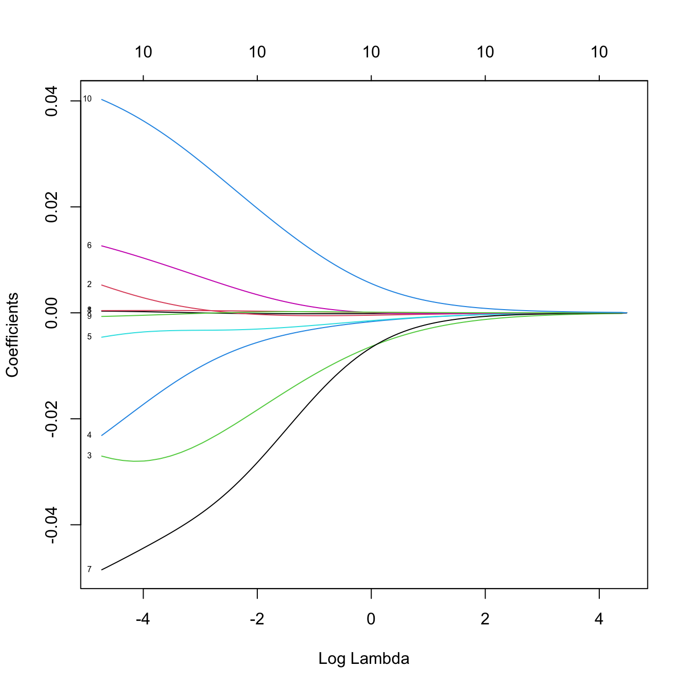
plot(lasso_mod, label = TRUE, xvar = "lambda")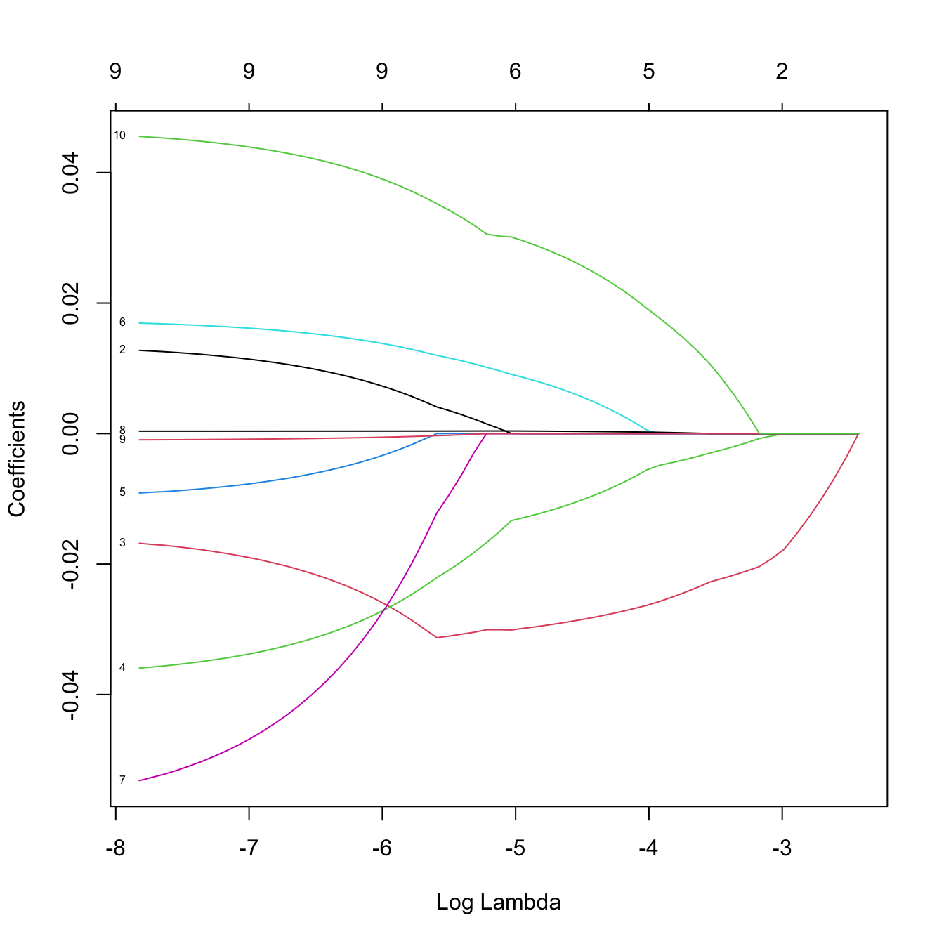
# Versus the percentage of deviance explained
plot(ridge_mod, label = TRUE, xvar = "dev")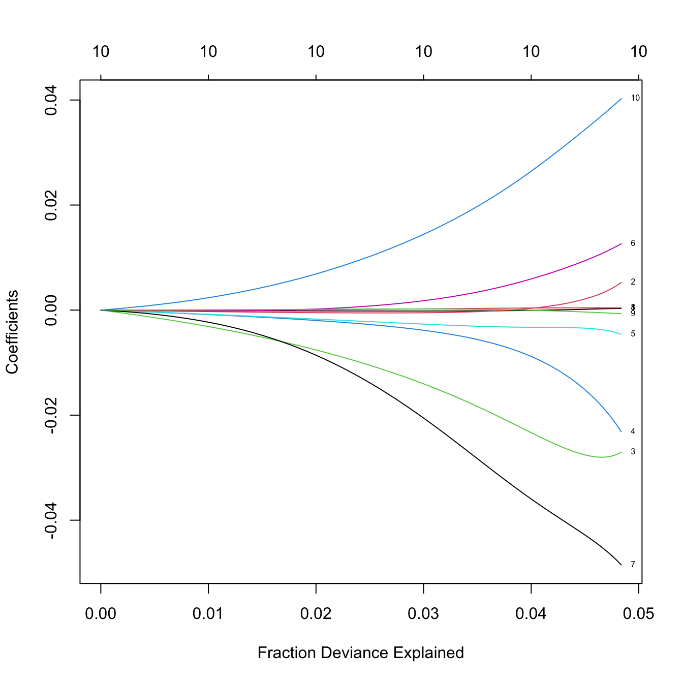
plot(lasso_mod, label = TRUE, xvar = "dev")
# The percentage of deviance explained only goes up to 0.05. There are no
# clear patterns indicating player differences between both leagues

# Let's select the predictors to be included with a 10-fold cross-validation
set.seed(12345)
kcv_lasso <- cv.glmnet(x = x, y = y, alpha = 1, nfolds = 10,
                       family = "binomial")
plot(kcv_lasso)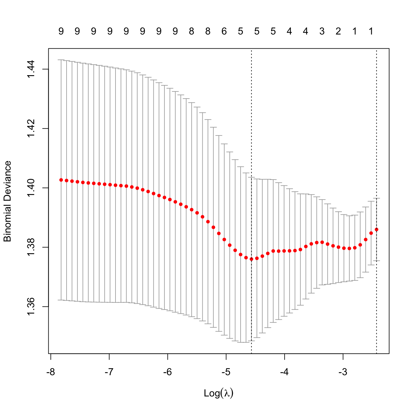
# The lambda that minimizes the CV error and "one standard error rule"'s lambda
kcv_lasso$lambda.min
## [1] 0.01039048
kcv_lasso$lambda.1se
## [1] 0.08829343

# Leave-one-out cross-validation -- similar result
ncv_lasso <- cv.glmnet(x = x, y = y, alpha = 1, nfolds = nrow(Hitters),
                       family = "binomial")
plot(ncv_lasso)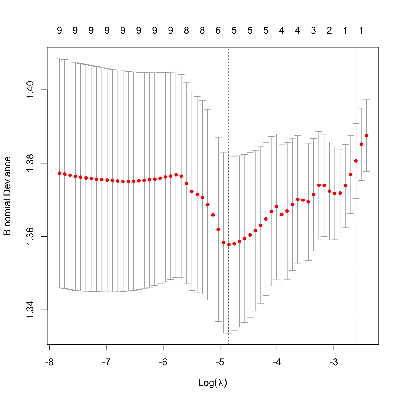
ncv_lasso$lambda.min
## [1] 0.007860015
ncv_lasso$lambda.1se
## [1] 0.07330276

# Model selected
coef(ncv_lasso, s = ncv_lasso$lambda.1se)
## 11 x 1 sparse Matrix of class "dgCMatrix"
##             s=0.07330276
## (Intercept) -0.099447861
## AtBat        .
## Hits         .
## HmRun       -0.006971231
## Runs         .
## RBI          .
## Walks        .
## DivisionW    .
## PutOuts      .
## Assists      .
## Errors       .
HmRun is selected by leave-one-out cross-validation as the unique predictor to be included in the lasso regression. We know that the model is not good due to the percentage of deviance explained. However, we still want to know whether HmRun has any significance at all. When addressing this, we have to take into account Appendix E to avoid spurious findings.
# Analyze the selected model
fit <- glm(League ~ HmRun, data = Hitters, family = "binomial")
summary(fit)
##
## Call:
## glm(formula = League ~ HmRun, family = "binomial", data = Hitters)
##
## Coefficients:
##             Estimate Std. Error z value Pr(>|z|)
## (Intercept)  0.27826    0.18086   1.539  0.12392
## HmRun       -0.04290    0.01371  -3.130  0.00175 **
## ---
## Signif. codes:  0 '***' 0.001 '**' 0.01 '*' 0.05 '.' 0.1 ' ' 1
##
## (Dispersion parameter for binomial family taken to be 1)
##
##     Null deviance: 443.95  on 321  degrees of freedom
## Residual deviance: 433.57  on 320  degrees of freedom
## AIC: 437.57
##
## Number of Fisher Scoring iterations: 4
# HmRun is significant -- but it may be spurious due to the model selection
# procedure (see Appendix A.5)

# Let's split the dataset in two, do model-selection in one part and then
# inference on the selected model in the other, to have an idea of the real
# significance of HmRun
set.seed(12345678)
train <- sample(c(FALSE, TRUE), size = nrow(Hitters), replace = TRUE)

# Model selection in training part
ncv_lasso <- cv.glmnet(x = x[train, ], y = y[train], alpha = 1,
                       nfolds = sum(train), family = "binomial")
coef(ncv_lasso, s = ncv_lasso$lambda.1se)
## 11 x 1 sparse Matrix of class "dgCMatrix"
##             s=0.08405683
## (Intercept)   0.27240020
## AtBat         .
## Hits          .
## HmRun        -0.01255322
## Runs          .
## RBI           .
## Walks         .
## DivisionW     .
## PutOuts       .
## Assists       .
## Errors        .

# Inference in testing part
summary(glm(League ~ HmRun, data = Hitters[!train, ], family = "binomial"))
##
## Call:
## glm(formula = League ~ HmRun, family = "binomial", data = Hitters[!train,
##     ])
##
## Coefficients:
##             Estimate Std. Error z value Pr(>|z|)
## (Intercept) -0.14389    0.25754  -0.559   0.5764
## HmRun       -0.03255    0.01955  -1.665   0.0958 .
## ---
## Signif. codes:  0 '***' 0.001 '**' 0.01 '*' 0.05 '.' 0.1 ' ' 1
##
## (Dispersion parameter for binomial family taken to be 1)
##
##     Null deviance: 216.54  on 162  degrees of freedom
## Residual deviance: 213.64  on 161  degrees of freedom
## AIC: 217.64
##
## Number of Fisher Scoring iterations: 4
# HmRun is now not significant...
# We can repeat the analysis for different partitions of the data and we will
# obtain weak significances. Therefore, we can conclude that this is a spurious
# finding and that HmRun is not significant as a single predictor

# Prediction (obviously not trustable, but for illustration)
pred <- predict(ncv_lasso, newx = x[!train, ], type = "response",
                s = ncv_lasso$lambda.1se)

# Hit matrix and hit ratio
H <- table(pred > 0.5, y[!train] == "A") # ("A" was the reference level)
H
##
##         FALSE TRUE
##   FALSE     5   18
##   TRUE     57   83
sum(diag(H)) / sum(H) # Almost like tossing a coin!
## [1] 0.5398773
From the above analysis, we can conclude that there are no significant differences between the players of both leagues in terms of the variables analyzed.
Exercise 5.8 Perform an adequate statistical analysis based on shrinkage of a generalized linear model to reply the following questions:
- What (if any) are the leading factors among the features of a player in season 1986 in order to be in the top \(10\%\) of most paid players in season 1987?
- What (if any) are the player features in season 1986 influencing the number of home runs in the same season? And during his career?
Hint: you may use the one shown in the section as a template.
For binary classification, cv.glmnet uses by default type.measure = "deviance" (the binomial deviance, \(-2\ell(\hat{\boldsymbol{\beta}})\)) as the CV loss. Two alternatives specifically tailored to classification are also available:
-
type.measure = "class": misclassification error rate, i.e., the proportion of observations wrongly classified using the \(0.5\) threshold on the predicted probabilities. This is the natural measure if the final goal is to minimize classification errors. -
type.measure = "auc": area under the ROC curve, a threshold-free measure of ranking performance. It requires enough observations of both classes within every fold (glmnetwarns if any fold has too few cases).
# Use type.measure = "class" instead of the default "deviance"
set.seed(12345)
kcv_lasso_class <- cv.glmnet(x = x, y = y, alpha = 1, nfolds = 10,
                             family = "binomial", type.measure = "class")
                             # type.measure = "auc" is a common alternative
plot(kcv_lasso_class) # y-axis now reports misclassification error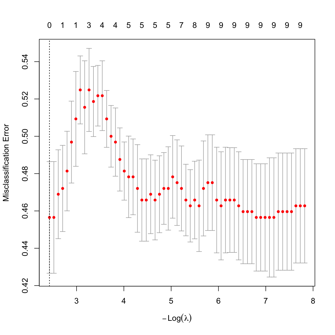
kcv_lasso_class$lambda.min
## [1] 0.08829343
kcv_lasso_class$lambda.1se
## [1] 0.08829343
# The optimal lambda may differ from the one selected with "deviance",
# since different CV losses can favor different amounts of regularization
5.9 Big data considerations
As we saw in Section 5.2.2, fitting a generalized linear model involves fitting a series of linear models. Therefore, all the memory problems that appeared in Section 4.4 are inherited. Worse, computation is now more complicated because:
- Computing the likelihood requires reading all the data at once. Differently from the linear model, updating the model with a new chunk implies re-fitting with all the data due to the nonlinearity of the likelihood.
- The IRLS algorithm requires reading the data as many times as iterations.
These two peculiarities are a game-changer for the approach followed in Section 4.4: biglm::bigglm needs to have access to the full data while performing the fitting. This can be cumbersome.
Hopefully, a neat solution is available using the ff and ffbase packages, which allow for efficiently “working with data stored in disk that behave (almost) as if they were in RAM”.191 The function that we will employ is ffbase::bigglm.ffdf, and requires an object of the class ffdf (ff’s data frames).
The latest version of ffbase has a bug in
ffbase::bigglm.ffdf that is reported in this GitHub issue.
Until that issue is solved, you will not be able to apply
ffbase::bigglm.ffdf with the latest package versions. A
temporary workaround is to downgrade the packages bit,
ff, and ffbase to the respective versions
1.1-15.2, 2.2-14.2, and 0.12.8.
The next two chunk of code provides this fix.
# To install specific versions of packages
install.packages("versions")
library(versions)

# Install specific package versions. It may take a while to do so, be patient
install.versions(pkgs = c("bit", "ff", "ffbase"),
                 versions = c("1.1-15.2", "2.2-14.2", "0.12.8"))
# After bit's version 1.1-15.2, something is off in the integration with
# ffbase; see issue in https://github.com/edwindj/ffbase/issues/61

# Alternatively, if the binaries for your OS are not available (e.g., for
# Apple M1's processors), then you will need to compile the packages from
# source... and cross your fingers!
urls <- c(
  "https://cran.r-project.org/src/contrib/Archive/bit/bit_1.1-15.2.tar.gz",
  "https://cran.r-project.org/src/contrib/Archive/ff/ff_2.2-14.2.tar.gz",
  "https://cran.r-project.org/src/contrib/Archive/ffbase/ffbase_0.12.8.tar.gz"
  )
install.packages(pkgs = urls, repos = NULL, type = "source")
After the packages bit, ff, and ffbase have been downgraded (or if the GitHub issue has been fixed), then you will be able to run the following code:
# Not really "big data", but for the sake of illustration
set.seed(12345)
n <- 1e6
p <- 10
beta <- seq(-1, 1, length.out = p)^5
x1 <- matrix(rnorm(n * p), nrow = n, ncol = p)
x1[, p] <- 2 * x1[, 1] + rnorm(n, sd = 0.1) # Add some dependence to predictors
x1[, p - 1] <- 2 - x1[, 2] + rnorm(n, sd = 0.5)
y1 <- rbinom(n, size = 1, prob = 1 / (1 + exp(-(1 + x1 %*% beta))))
x2 <- matrix(rnorm(100 * p), nrow = 100, ncol = p)
y2 <- rbinom(100, size = 1, prob = 1 / (1 + exp(-(1 + x2 %*% beta))))
big_data1 <- data.frame("resp" = y1, "pred" = x1)
big_data2 <- data.frame("resp" = y2, "pred" = x2)

# Save files to disk to emulate the situation with big data
write.csv(x = big_data1, file = "bigData1.csv", row.names = FALSE)
write.csv(x = big_data2, file = "bigData2.csv", row.names = FALSE)

# Read files using ff
library(ffbase) # Imports ff
big_data1ff <- read.table.ffdf(file = "bigData1.csv", header = TRUE, sep = ",")
big_data2ff <- read.table.ffdf(file = "bigData2.csv", header = TRUE, sep = ",")

# Recall: bigData1.csv is not copied into RAM
print(object.size(big_data1), units = "MB")
print(object.size(big_data1ff), units = "KB")

# Logistic regression
# Same comments for the formula framework -- this is the hack for automatic
# inclusion of all the predictors
library(biglm)
f <- formula(paste("resp ~", paste(names(big_data1)[-1], collapse = " + ")))
bigglm_mod <- bigglm.ffdf(formula = f, data = big_data1ff, family = binomial())

# glm's call
glm_mod <- glm(formula = resp ~ ., data = big_data1, family = binomial())

# Compare sizes
print(object.size(bigglm_mod), units = "KB")
print(object.size(glm_mod), units = "MB")

# Summaries
s1 <- summary(bigglm_mod)
s2 <- summary(glm_mod)
s1
s2

# Further information
s1$mat # Coefficients and their inferences
s1$rsq # R^2
s1$nullrss # Null deviance

# Extract coefficients
coef(bigglm_mod)

# Prediction works as usual
predict(bigglm_mod, newdata = big_data2[1:5, ], type = "response")
# predict(bigglmMod, newdata = bigData2[1:5, -1]) # Error

# Update the model with training data
update(bigglm_mod, moredata = big_data2)

# AIC and BIC
AIC(bigglm_mod, k = 2)
AIC(bigglm_mod, k = log(n))

# Delete the files in disk
file.remove(c("bigData1.csv", "bigData2.csv"))
Note that this is also a perfectly valid approach for linear
models, we just need to specify
family = gaussian() in the call to
bigglm.ffdf.
Model selection of biglm::bigglm models is not so straightforward. The trick that leaps::regsubsets employs for simplifying the model search in linear models (see Section 4.4) does not apply for generalized linear models because of the nonlinearity of the likelihood. However, there is a simple and useful hack: we can do best subset selection in the linear model associated with the last iteration of the IRLS algorithm and then refine the search by computing the exact BIC/AIC from a set of candidate models.192 If we do so, we translate the model selection problem back to the linear case, plus an extra overhead of fitting several generalized linear models. Keep in mind that, albeit useful, this approach is a hacky approximation to the task of finding the best subset of predictors.
# Model selection adapted to big data generalized linear models
reg <- leaps::regsubsets(bigglm_mod, nvmax = p + 1, method = "exhaustive")
# This takes the QR decomposition, which encodes the linear model associated
# with the last iteration of the IRLS algorithm. However, the reported BICs are
# *not* the true BICs of the generalized linear models, but a sufficient
# approximation to obtain a list of candidate models in a fast way

# Get the model with lowest BIC
plot(reg)
subs <- summary(reg)
subs$which
subs$bic
subs$which[which.min(subs$bic), ]

# Let's compute the true BICs for the p models. This implies fitting p bigglm's
best_models <- list()
for (i in 1:nrow(subs$which)) {
  f <- formula(paste("resp ~", paste(names(which(subs$which[i, -1])),
                                     collapse = " + ")))
  best_models[[i]] <- bigglm.ffdf(formula = f, data = big_data1ff,
                                  family = binomial(), maxit = 20)
  # Did not converge with the default iteration limit, maxit = 8

}

# The approximate BICs and the true BICs are very similar (in this example)
exact_bi_cs <- sapply(best_models, AIC, k = log(n))
plot(subs$bic, exact_bi_cs, type = "o", xlab = "Exact", ylab = "Approximate")

# Pearson correlation
cor(subs$bic, exact_bi_cs, method = "pearson")

# Order correlation
cor(subs$bic, exact_bi_cs, method = "spearman")

# Both give the same model selection and same order
subs$which[which.min(subs$bic), ] # Approximate
subs$which[which.min(exact_bi_cs), ] # Exact
References
His Appendix F in the Rogers Commission is particularly critical on the increasing sequence of risks that NASA took previously to the Challenger disaster. His closing sentence: “For a successful technology, reality must take precedence over public relations, for nature cannot be fooled”.↩︎
Episode S1:E3 “A Major Malfunction” in Netflix’s series “Challenger: The Final Flight” reproduces the events during this teleconference between Thiokol (Promontory, Utah) and NASA (Cape Canaveral, Florida), with interviews to the relevant actors. The coverage of the teleconference spans from the time marks 17:40 to 23:55. Relevant highlights are: the engineers are told to give an assessment of concerns regarding launching in cold weather (17:40–18:56); the engineers present the report and their unquantified concerns about higher risk with cold temperatures (20:38–21:20); Larry Mulloy, NASA manager in 1986, says “The data [the engineers presented] did not support the recommendation that the engineers were making. The data was totally inconclusive.” (21:47–21:58); the vice president of engineers of Thiokol, Robert Lund, gives the specific recommendation to not launch below \(53\) degrees Fahrenheit (\(11.67\) degrees Celsius) and Larry Mulloy replies (22:33–22:53); Robert Lund, pressured, changes his assessment and agrees with Larry Mulloy’s: data is inconclusive (24:12–25:33). Recall that the data presented during the teleconference is the one summarized in Figure 5.3a.↩︎
After the shuttle exits the atmosphere, the solid rocket boosters separate and descend to land using a parachute. After recovery, they are carefully analyzed.↩︎
Recall that a binomial variable with size \(n\) and probability \(p\), \(\mathrm{B}(n,p),\) is obtained by summing \(n\) independent \(\mathrm{Ber}(p),\) so \(\mathrm{Ber}(p)\) is the same distribution as \(\mathrm{B}(1,p).\)↩︎
Do not confuse this \(p\) with the number of predictors in the model, represented by \(p.\) The context should make unambiguous the use of \(p.\)↩︎
The fact that the logistic function is a cdf allows remembering that the logistic is to be applied to map \(\mathbb{R}\) into \([0,1],\) as opposed to the logit function.↩︎
And also, as we will see later, because it is the canonical link function.↩︎
Consequently, the name “odds” used in this context is singular, as it refers to a single ratio.↩︎
Recall that (traditionally) the result of a bet is binary: one either wins or loses it.↩︎
For example, if a horse \(Y\) has probability \(p=2/3\) of winning a race (\(Y=1\)), then the odds of the horse is \(\frac{p}{1-p}=\frac{2/3}{1/3}=2.\) This means that the horse has a probability of winning that is twice larger than the probability of losing. This is sometimes written as a \(2:1\) or \(2 \times 1\) (spelled “two-to-one”).↩︎
For the previous example: if the odds of the horse was \(5,\) then the probability of winning would be \(p=5/6.\)↩︎
As in the linear model, we assume the randomness comes from the error present in \(Y\) once \(\mathbf{X}\) is given, not from the \(\mathbf{X},\) and we therefore denote \(\mathbf{x}_i\) to the \(i\)-th observation of \(\mathbf{X}.\)↩︎
Section 5.7 discusses in detail the assumptions of generalized linear models.↩︎
Notice that this approach is very different from directly transforming the response as \(g(Y),\) as outlined in Section 3.5.1. Indeed, in generalized linear models one transforms \(\mathbb{E}[Y \mid X_1,\ldots,X_p],\) not \(Y.\) Of course, \(g(\mathbb{E}[Y \mid X_1,\ldots,X_p])\neq \mathbb{E}[g(Y) \mid X_1,\ldots,X_p].\)↩︎
Not to be confused with the exponential distribution \(\mathrm{Exp}(\lambda),\) which is a member of the exponential family.↩︎
This is the so-called canonical form of the exponential family. Generalizations of the family are possible, though we do not consider them.↩︎
The pdf of a \(\Gamma(a,\nu)\) is \(f(x;a,\nu)=\frac{a^\nu}{\Gamma(\nu)}x^{\nu-1}e^{-ax},\) for \(a,\nu>0\) and \(x\in(0,\infty)\) (the pdf is zero otherwise). The expectation is \(\mathbb{E}\lbrack\Gamma(a,\nu)\rbrack=\frac{\nu}{a}.\)↩︎
If the argument \(-\eta \nu\) is not positive, then the probability assigned by \(\Gamma(-\eta \nu,\nu)\) is zero. This delicate case may complicate the estimation of the model. Valid starting values for \(\boldsymbol{\beta}\) are required.↩︎
Note that this situation is very different from logistic regression, for which we either have observations with the values \(0\) or \(1.\) In binomial regression, we can naturally have proportions.↩︎
Clearly, \(\mathbb{E}[\mathrm{B}(N,p)/N]=p\) because \(\mathbb{E}[\mathrm{B}(N,p)]=Np.\)↩︎
The sample size here is \(n=12,\) not \(226.\) There are \(N_{1},\ldots,N_{12}\) binomial sizes corresponding to each observation, and \(\sum_{i=1}^{n}N_i=226.\)↩︎
We assume the randomness comes from the error present in \(Y\) once \(\mathbb{X}\) is given, not from the \(\mathbb{X}.\) This is implicit in the considered expectations.↩︎
The system stems from a first-order Taylor expansion of the function \(\frac{\partial \ell(\boldsymbol{\beta})}{\partial \boldsymbol{\beta}}:\mathbb{R}^{p+1}\rightarrow\mathbb{R}^{p+1}\) about the root \(\hat{\boldsymbol{\beta}},\) where \(\left.\frac{\partial \ell(\boldsymbol{\beta})}{\partial \boldsymbol{\beta}} \right |_{\boldsymbol{\beta}=\hat{\boldsymbol{\beta}}}=\mathbf{0}.\)↩︎
Recall that \(\mathbb{E}[(Y_i-\mu_i)(Y_j-\mu_j)]=\mathrm{Cov}[Y_i,Y_j]=\begin{cases}V_i,&i=j,\\0,&i\neq j,\end{cases}\) because of independence.↩︎
That work quite well in practice and deliver many valuable insights.↩︎
The linear model is an exception in terms of exact and simple inference, not the rule.↩︎
Recall expression (5.23) for the general case of \(\mathcal{I}(\boldsymbol{\beta}).\)↩︎
Understood as small \(|(\mathbb{X}^\top\mathbf{V}\mathbb{X})^{-1}|.\)↩︎
Because \(e^{\hat\beta_j-\hat{\mathrm{SE}}(\hat\beta_j)z_{\alpha/2}}\leq e^{\beta_j}\leq e^{\hat\beta_j+\hat{\mathrm{SE}}(\hat\beta_j)z_{\alpha/2}}\iff \hat\beta_j-\hat{\mathrm{SE}}(\hat\beta_j)z_{\alpha/2}\leq \beta_j \leq\hat\beta_j+\hat{\mathrm{SE}}(\hat\beta_j)z_{\alpha/2}\) since the exponential is a monotone increasing function.↩︎
For example, the CI for the conditional response in the logistic model is not very informative, as it can either be \(\{0\},\) \(\{1\}\) or \(\{0,1\}.\) Predictions and CIs for the conditional response are carried out on a model-by-model basis.↩︎
Whether at this temperature it would have been a fatal incident or not is left to speculation.↩︎
This model is not necessarily the model that best generalizes. Just the one that better explains the (training) sample.↩︎
Several are possible depending on the interpolation between points.↩︎
The canonical link function \(g\) is the identity, check (5.12) and (5.13).↩︎
Note that \(D_{p_1}^*>D^*_{p_2}\) because \(\ell(\hat{\boldsymbol{\beta}}_{p_1})<\ell(\hat{\boldsymbol{\beta}}_{p_2}).\)↩︎
In other words, \(M_2\) does not add significant predictors when compared with the submodel \(M_1.\)↩︎
The
leapspackage does not support generalized linear models directly. There are, however, other packages for performing best subset selection with generalized linear models, but we do not cover them here.↩︎This is a common way of generating a binary variable from a quantitative variable.↩︎
Also, due to the variety of ranges the response \(Y\) is allowed to take in generalized linear models.↩︎
The logic behind the statement is that a \(\chi^2_k\) random variable has the same distribution as the sum of \(k\) independent squared \(\mathcal{N}(0,1)\) variables.↩︎
Practical counterexamples to the statement are possible, see Figures 5.16 and 5.18.↩︎
This would be the rigorous approach, but it is notably more complex.↩︎
We are now minimizing \(-\ell(\boldsymbol{\beta}),\) the negative log-likelihood.↩︎
The
ffpackage implements theffvectors andffdfdata frames classes. The packageffbaseprovides convenience functions for working with these non-standard classes in a more transparent way.↩︎Without actually expanding that list, as coming up with this list of candidate models is the most expensive part in best subset selection.↩︎