1 Introduction

1.1 What is Predictive Modeling?

Predictive modeling is the process of developing a mathematical tool or model that generates an accurate prediction about a random quantity of interest.

In predictive modeling we are interested in predicting a random variable, typically denoted by $Y,$ from a set of related variables $X_1,\ldots,X_p.$ The focus is on learning what is the probabilistic model that relates $Y$ with $X_1,\ldots,X_p,$ and use that acquired knowledge for predicting $Y$ given an observation of $X_1,\ldots,X_p.$ Some concrete examples of this are:

Predicting the wine quality ($Y$) from a set of environmental variables ($X_1,\ldots,X_p$).
Predicting the number of sales ($Y$) from a set of marketing investments ($X_1,\ldots,X_p$).
Modeling the average house value in a given suburb ($Y$) from a set of community-related features ($X_1,\ldots,X_p$).
Predicting the probability of failure ($Y$) of a rocket launcher from the ambient temperature ($X_1$).
Predicting students’ academic performance ($Y$) according to education resources and learning methodologies ($X_1,\ldots,X_p$).
Predicting the fuel consumption of a car ($Y$) from a set of driving variables ($X_1,\ldots,X_p$).

The process of predictive modeling can be statistically abstracted in the following way. We believe that $Y$ and $X_1,\ldots,X_p$ are related by a regression model of the form

\[\begin{align} Y=m(X_1,\ldots,X_p)+\varepsilon,\tag{1.1} \end{align}\]

where $m$ is the regression function and $\varepsilon$ is a random error with zero mean that accounts for the uncertainty of knowing $Y$ if $X_1,\ldots,X_p$ are known. The function $m:\mathbb{R}^p\rightarrow\mathbb{R}$ is unknown in practice and its estimation is the objective of predictive modeling: $m$ encodes the relation² between $Y$ and $X_1,\ldots,X_p$. In other words, $m$ captures the trend of the relation between $Y$ and $X_1,\ldots,X_p,$ and $\varepsilon$ represents the stochasticity of that relation. Knowing $m$ allows predicting $Y.$ This course is devoted to statistical models³ that allow us to come up with an estimate of $m,$ denoted by $\hat m,$ that can be used to predict $Y.$

Let’s see a concrete example of this with an artificial dataset. Suppose $Y$ represents average fuel consumption (l/100km) of a car and $X$ is the average speed (km/h). It is well-known from physics that the energy and speed have a quadratic relationship, and therefore we may assume that $Y$ and $X$ are truly quadratically-related for the sake of exposition:

\[\begin{align*} Y=a+bX+cX^2+\varepsilon. \end{align*}\]

Then $m:\mathbb{R}\rightarrow\mathbb{R}$ ($p=1$) with $m(x)=a+bx+cx^2.$ Suppose the following data consists of measurements from a given car model, measured in different drivers and conditions (we do not have data for accounting for all those effects, which go to the $\varepsilon$ term⁴):

x <- c(64, 20, 14, 64, 44, 39, 25, 53, 48, 9, 100, 112, 78, 105, 116, 94, 71,
       71, 101, 109)
y <- c(4, 6, 6.4, 4.1, 4.9, 4.4, 6.6, 4.4, 3.8, 7, 7.4, 8.4, 5.2, 7.6, 9.8,
       6.4, 5.1, 4.8, 8.2, 8.7)
plot(x, y, xlab = "Speed", ylab = "Fuel consumption")

Figure 1.1: Scatterplot of fuel consumption vs. speed.

From this data, we can estimate $m$ by means of a polynomial model⁵:

# Estimates for a, b, and c
lm(y ~ x + I(x^2))
## 
## Call:
## lm(formula = y ~ x + I(x^2))
## 
## Coefficients:
## (Intercept)            x       I(x^2)  
##    8.512421    -0.153291     0.001408

Then the estimate of $m$ is $\hat m(x)=\hat{a}+\hat{b} x+\hat{c} x^2=8.512-0.153x+0.001x^2$ and its fit to the data is pretty good. As a consequence, we can use this precise mathematical function to predict the $Y$ from a particular observation $X.$ For example, the estimated fuel consumption at speed 90 km/h is 8.512421 - 0.153291 * 90 + 0.001408 * 90^2 = 6.1210.

plot(x, y, xlab = "Speed", ylab = "Fuel consumption")
curve(8.512421 - 0.153291 * x + 0.001408 * x^2, add = TRUE, col = 2)

Figure 1.2: Fitted quadratic model.

There are a number of generic issues and decisions to take when building and estimating regression models that are worth highlighting:

The prediction accuracy versus interpretability trade-off. Prediction accuracy is key in any predictive model: of course, the better the model is able to predict $Y,$ the more useful it will be. However, some models achieve this predictive accuracy in exchange for a clear interpretability of the model (the so-called black boxes). Interpretability is key in order to gain insights on the prediction process, to know exactly which variables are most influential in $Y,$ to be able to interpret the parameters of the model, and to translate the prediction process to non-experts. In essence, interpretability allows to explain precisely how and why the model behaves when predicting $Y$ from $X_1,\ldots,X_p.$ Most of the models covered in this text clearly favor interpretability⁶ and hence they may make a sacrifice in terms of their prediction accuracy when compared with more convoluted models.
Model correctness versus model usefulness. Correctness and usefulness are two different concepts in modeling. The first refers to the model being statistically correct, that is, it translates to stating that the assumptions on which the model relating $Y$ with $X_1,\ldots,X_p$ is built are satisfied. The second refers to the model being useful for explaining or predicting $Y$ from $X_1,\ldots,X_p.$ Both concepts are certainly related (if the model is correct/useful, then likely it is useful/correct) but neither is implied by the other. For example, a regression model might be correct but useless if the variance of $\varepsilon$ is large (too much noise). And yet if the model is not completely correct, it may give useful insights and predictions, but inference may be completely spurious.⁷
Flexibility versus simplicity. The best model is the one which is very simple (low number of parameters), highly interpretable, and delivers great predictions. This is often unachievable in practice. What can be achieved is a good model: the one that balances the simplicity with the prediction accuracy, which is often increased the more flexible the model is. However, flexibility comes at a price: more flexible (hence more complex) models use more parameters that need to be estimated from a finite amount of information – the sample. This is problematic, as overly flexible models are more dependent on the sample, up to the point in which they end up not estimating the true relation between $Y$ and $X_1,\ldots,X_p,$ $m,$ but merely interpolating the observed data. This well-known phenomenon is called overfitting and it can be avoided by splitting the dataset in two datasets:⁸ the training dataset, used for estimating the model; and the testing dataset, used for evaluating the fitted model predictive performance. On the other hand, excessive simplicity (underfitting) is also problematic, since the true relation between $Y$ and $X_1,\ldots,X_p$ may be overly simplified. Therefore, a trade-off in the degree of flexibility has to be attained to have a good model. This is often referred to as the bias-variance trade-off (low flexibility increases the bias of the fitted model, high flexibility increases the variance). An illustration of this transversal problem in predictive modeling is given in Figure 1.3.

Figure 1.3: Illustration of overfitting in polynomial regression. The left plot shows the training dataset and the right plot the testing dataset. Better fitting of the training data with a higher polynomial order does not imply better performance in new observations (prediction), but just an over-fitting of the available data with an overly-parametrized model (too flexible for the amount of information available). Reduction in the predictive error is only achieved with fits (in red) of polynomial degrees close to the true regression (in black). Application available here.

1.2 General notation and background

We use capital letters to denote random variables, such as $X,$ and lowercase, such as $x,$ to denote deterministic values. For example $\mathbb{P}[X=x]$ means “the probability that the random variable $X$ takes the particular value $x$”. In predictive modeling we are concerned about the prediction or explanation of a response $Y$ from a set of predictors $X_1,\ldots,X_p.$ Both $Y$ and $X_1,\ldots,X_p$ are random variables, but we use them in a different way: our interest lies in predicting or explaining $Y$ from $X_1,\ldots,X_p.$ Another name for $Y$ is dependent variable and $X_1,\ldots,X_p$ are sometimes referred to as independent variables, covariates, or explanatory variables. We will not use these terminologies.

The cumulative distribution function (cdf) of a random variable $X$ is $F(x):=\mathbb{P}[X\leq x]$ and is a function that completely characterizes the randomness of $X.$ Continuous random variables are also characterized by the probability density function (pdf) $f(x)=F'(x),$⁹ which represents the infinitesimal relative probability of $X$ per unit of length. On the other hand, discrete random variables are also characterized by the probability mass function $\mathbb{P}[X= x].$ We write $X\sim F$ (or $X\sim f$ if $X$ is continuous) to denote that $X$ has a cdf $F$ (or a pdf $f$). If two random variables $X$ and $Y$ have the same distribution, we write $X\stackrel{d}{=}Y.$

For a random variable $X\sim F,$ the expectation of $g(X)$ is defined as¹⁰

\[\begin{align*} \mathbb{E}[g(X)]:=&\,\int g(x)\,\mathrm{d}F(x)\\ :=&\, \begin{cases} \displaystyle\int g(x)f(x)\,\mathrm{d}x,&\text{ if }X\text{ is continuous,}\\\displaystyle\sum_{\{x\in\mathbb{R}:\mathbb{P}[X=x]>0\}} g(x)\mathbb{P}[X=x],&\text{ if }X\text{ is discrete.} \end{cases} \end{align*}\]

The sign “$:=$” emphasizes that the Left Hand Side (LHS) of the equality is defined for the first time as the Right Hand Side (RHS). Unless otherwise stated, the integration limits of any integral are $\mathbb{R}$ or $\mathbb{R}^p.$ The variance is defined as $\mathbb{V}\mathrm{ar}[X]:=\mathbb{E}[(X-\mathbb{E}[X])^2]=\mathbb{E}[X^2]-\mathbb{E}[X]^2.$

We employ boldface to denote vectors (assumed to be column matrices, although sometimes written in row-layout), like $\mathbf{a},$ and matrices, like $\mathbf{A}.$ We use $\mathbf{A}^\top$ to denote the transpose of $\mathbf{A}.$ Boldfaced capitals will be used simultaneously for denoting matrices and also random vectors $\mathbf{X}=(X_1,\ldots,X_p),$ which are collections of random variables $X_1,\ldots,X_p.$ The (joint) cdf of $\mathbf{X}$ is¹¹

\[\begin{align*} F(\mathbf{x}):=\mathbb{P}[\mathbf{X}\leq \mathbf{x}]:=\mathbb{P}[X_1\leq x_1,\ldots,X_p\leq x_p] \end{align*}\]

and, if $\mathbf{X}$ is continuous, its (joint) pdf is $f:=\frac{\partial^p}{\partial x_1\cdots\partial x_p}F.$

The marginals of $F$ and $f$ are the cdf and pdf of $X_j,$ $j=1,\ldots,p,$ respectively. They are defined as:

\[\begin{align*} F_{X_j}(x_j)&:=\mathbb{P}[X_j\leq x_j]=F(\infty,\ldots,\infty,x_j,\infty,\ldots,\infty),\\ f_{X_j}(x_j)&:=\frac{\partial}{\partial x_j}F_{X_j}(x_j)=\int_{\mathbb{R}^{p-1}} f(\mathbf{x})\,\mathrm{d}\mathbf{x}_{-j}, \end{align*}\]

where $\mathbf{x}_{-j}:=(x_1,\ldots,x_{j-1},x_{j+1},\ldots,x_p).$ The definitions can be extended analogously to the marginals of the cdf and pdf of different subsets of $\mathbf{X}.$

The conditional cdf and pdf of $X_1 \mid (X_2,\ldots,X_p)$ are defined, respectively, as

\[\begin{align*} F_{X_1 \mid \mathbf{X}_{-1}=\mathbf{x}_{-1}}(x_1)&:=\mathbb{P}[X_1\leq x_1 \mid \mathbf{X}_{-1}=\mathbf{x}_{-1}],\\ f_{X_1 \mid \mathbf{X}_{-1}=\mathbf{x}_{-1}}(x_1)&:=\frac{f(\mathbf{x})}{f_{\mathbf{X}_{-1}}(\mathbf{x}_{-1})}. \end{align*}\]

The conditional expectation of $Y \mid X$ is the following random variable¹²

\[\begin{align*} \mathbb{E}[Y \mid X]:=\int y \,\mathrm{d}F_{Y \mid X}(y \mid X). \end{align*}\]

For two random variables $X_1$ and $X_2,$ the covariance between them is defined as

\[\begin{align*} \mathrm{Cov}[X_1,X_2]:=\mathbb{E}[(X_1-\mathbb{E}[X_1])(X_2-\mathbb{E}[X_2])]=\mathbb{E}[X_1X_2]-\mathbb{E}[X_1]\mathbb{E}[X_2], \end{align*}\]

and the correlation between them is defined as

\[\begin{align*} \mathrm{Cor}[X_1,X_2]:=\frac{\mathrm{Cov}[X_1,X_2]}{\sqrt{\mathbb{V}\mathrm{ar}[X_1]\mathbb{V}\mathrm{ar}[X_2]}}. \end{align*}\]

The variance and the covariance are extended to a random vector $\mathbf{X}=(X_1,\ldots,X_p)^\top$ by means of the so-called variance-covariance matrix:

\[\begin{align*} \mathbb{V}\mathrm{ar}[\mathbf{X}]:=&\,\mathbb{E}[(\mathbf{X}-\mathbb{E}[\mathbf{X}])(\mathbf{X}-\mathbb{E}[\mathbf{X}])^\top]\\ =&\,\mathbb{E}[\mathbf{X}\mathbf{X}^\top]-\mathbb{E}[\mathbf{X}]\mathbb{E}[\mathbf{X}]^\top\\ =&\,\begin{pmatrix} \mathbb{V}\mathrm{ar}[X_1] & \mathrm{Cov}[X_1,X_2] & \cdots & \mathrm{Cov}[X_1,X_p]\\ \mathrm{Cov}[X_2,X_1] & \mathbb{V}\mathrm{ar}[X_2] & \cdots & \mathrm{Cov}[X_2,X_p]\\ \vdots & \vdots & \ddots & \vdots \\ \mathrm{Cov}[X_p,X_1] & \mathrm{Cov}[X_p,X_2] & \cdots & \mathbb{V}\mathrm{ar}[X_p]\\ \end{pmatrix}, \end{align*}\]

where $\mathbb{E}[\mathbf{X}]:=(\mathbb{E}[X_1],\ldots,\mathbb{E}[X_p])^\top$ is just the componentwise expectation. As in the univariate case, the expectation is a linear operator, which now means that

\[\begin{align} \mathbb{E}[\mathbf{A}\mathbf{X}+\mathbf{b}]=\mathbf{A}\mathbb{E}[\mathbf{X}]+\mathbf{b},\quad\text{for a $q\times p$ matrix } \mathbf{A}\text{ and }\mathbf{b}\in\mathbb{R}^q.\tag{1.2} \end{align}\]

It follows from (1.2) that

\[\begin{align} \mathbb{V}\mathrm{ar}[\mathbf{A}\mathbf{X}+\mathbf{b}]=\mathbf{A}\mathbb{V}\mathrm{ar}[\mathbf{X}]\mathbf{A}^\top,\quad\text{for a $q\times p$ matrix } \mathbf{A}\text{ and }\mathbf{b}\in\mathbb{R}^q.\tag{1.3} \end{align}\]

The $p$-dimensional normal of mean $\boldsymbol{\mu}\in\mathbb{R}^p$ and covariance matrix $\boldsymbol{\Sigma}$ (a $p\times p$ symmetric and positive definite matrix) is denoted by $\mathcal{N}_{p}(\boldsymbol{\mu},\boldsymbol{\Sigma})$ and is the generalization to $p$ random variables of the usual normal distribution. Its (joint) pdf is given by

\[\begin{align*} \phi(\mathbf{x};\boldsymbol{\mu},\boldsymbol{\Sigma}):=\frac{1}{(2\pi)^{p/2}|\boldsymbol{\Sigma}|^{1/2}}e^{-\frac{1}{2}(\mathbf{x}-\boldsymbol{\mu})^\top\boldsymbol{\Sigma}^{-1}(\mathbf{x}-\boldsymbol{\mu})},\quad \mathbf{x}\in\mathbb{R}^p. \end{align*}\]

The $p$-dimensional normal has a nice linear property that stems from (1.2) and (1.3):

\[\begin{align} \mathbf{A}\mathcal{N}_p(\boldsymbol\mu,\boldsymbol\Sigma)+\mathbf{b}\stackrel{d}{=}\mathcal{N}_q(\mathbf{A}\boldsymbol\mu+\mathbf{b},\mathbf{A}\boldsymbol\Sigma\mathbf{A}^\top).\tag{1.4} \end{align}\]

Notice that when $p=1,$ and $\boldsymbol{\mu}=\mu$ and $\boldsymbol{\Sigma}=\sigma^2,$ then the pdf of the usual normal $\mathcal{N}(\mu,\sigma^2)$ is recovered:¹³

\[\begin{align*} \phi(x;\mu,\sigma^2):=\frac{1}{\sqrt{2\pi}\sigma}e^{-\frac{(x-\mu)^2}{2\sigma^2}}. \end{align*}\]

When $p=2,$ the pdf is expressed in terms of $\boldsymbol{\mu}=(\mu_1,\mu_2)^\top$ and $\boldsymbol{\Sigma}=(\sigma_1^2,\rho\sigma_1\sigma_2;\rho\sigma_1\sigma_2,\sigma_2^2),$ for $\mu_1,\mu_2\in\mathbb{R},$ $\sigma_1,\sigma_2>0,$ and $-1<\rho<1$:

\[\begin{align} &\phi(x_1,x_2;\mu_1,\mu_2,\sigma_1^2,\sigma_2^2,\rho):=\frac{1}{2\pi\sigma_1\sigma_2\sqrt{1-\rho^2}}\tag{1.5}\\ &\;\times\exp\left\{-\frac{1}{2(1-\rho^2)}\left[\frac{(x_1-\mu_1)^2}{\sigma_1^2}+\frac{(x_2-\mu_2)^2}{\sigma_2^2}-\frac{2\rho(x_1-\mu_1)(x_2-\mu_2)}{\sigma_1\sigma_2}\right]\right\}.\nonumber \end{align}\]

The surface defined by (1.5) can be regarded as a $3$-dimensional bell. In addition, it serves to provide concrete examples of the functions introduced above:

Joint pdf:

\[\begin{align*} f(x_1,x_2)=\phi(x_1,x_2;\mu_1,\mu_2,\sigma_1^2,\sigma_2^2,\rho). \end{align*}\]
Marginal pdfs:

\[\begin{align*} f_{X_1}(x_1)=\int \phi(x_1,t_2;\mu_1,\mu_2,\sigma_1^2,\sigma_2^2,\rho)\,\mathrm{d}t_2=\phi(x_1;\mu_1,\sigma_1^2) \end{align*}\]

and $f_{X_2}(x_2)=\phi(x_2;\mu_2,\sigma_2^2).$ Hence $X_1\sim\mathcal{N}\left(\mu_1,\sigma_1^2\right)$ and $X_2\sim\mathcal{N}\left(\mu_2,\sigma_2^2\right).$
Conditional pdfs:

\[\begin{align*} f_{X_1 \mid X_2=x_2}(x_1)=&\frac{f(x_1,x_2)}{f_{X_2}(x_2)}=\phi\left(x_1;\mu_1+\rho\frac{\sigma_1}{\sigma_2}(x_2-\mu_2),(1-\rho^2)\sigma_1^2\right),\\ f_{X_2 \mid X_1=x_1}(x_2)=&\phi\left(x_2;\mu_2+\rho\frac{\sigma_2}{\sigma_1}(x_1-\mu_1),(1-\rho^2)\sigma_2^2\right). \end{align*}\]

Hence

\[\begin{align*} X_1& \mid X_2=x_2\sim\mathcal{N}\left(\mu_1+\rho\frac{\sigma_1}{\sigma_2}(x_2-\mu_2),(1-\rho^2)\sigma_1^2\right),\\ X_2& \mid X_1=x_1\sim\mathcal{N}\left(\mu_2+\rho\frac{\sigma_2}{\sigma_1}(x_1-\mu_1),(1-\rho^2)\sigma_2^2\right). \end{align*}\]
Conditional expectations:

\[\begin{align*} \mathbb{E}[X_1 \mid X_2=x_2]&=\mu_1+\rho\frac{\sigma_1}{\sigma_2}(x_2-\mu_2),\\ \mathbb{E}[X_2 \mid X_1=x_1]&=\mu_2+\rho\frac{\sigma_2}{\sigma_1}(x_1-\mu_1). \end{align*}\]
Joint cdf:

\[\begin{align*} \int_{-\infty}^{x_2}\int_{-\infty}^{x_1}\phi(t_1,t_2;\mu_1,\mu_2,\sigma_1^2,\sigma_2^2,\rho)\,\mathrm{d}t_1\,\mathrm{d}t_2. \end{align*}\]
Marginal cdfs: $\int_{-\infty}^{x_1}\phi(t;\mu_1,\sigma_1^2)\,\mathrm{d}t=:\Phi(x_1;\mu_1,\sigma_1^2)$ and analogously $\Phi(x_2;\mu_2,\sigma_2^2).$
Conditional cdfs:

\[\begin{align*} \int_{-\infty}^{x_1}\phi\left(t;\mu_1+\rho\frac{\sigma_1}{\sigma_2}(x_2-\mu_2),(1-\rho^2)\sigma_1^2\right)\,\mathrm{d}t=\Phi\left(x_1;\mu_1+\rho\frac{\sigma_1}{\sigma_2}(x_2-\mu_2),(1-\rho^2)\sigma_1^2\right) \end{align*}\]

and analogously $\Phi\left(x_2;\mu_2+\rho\frac{\sigma_2}{\sigma_1}(x_1-\mu_1),(1-\rho^2)\sigma_2^2\right).$

Figure 1.4 graphically summarizes the concepts of joint, marginal, and conditional distributions within the context of a $2$-dimensional normal.

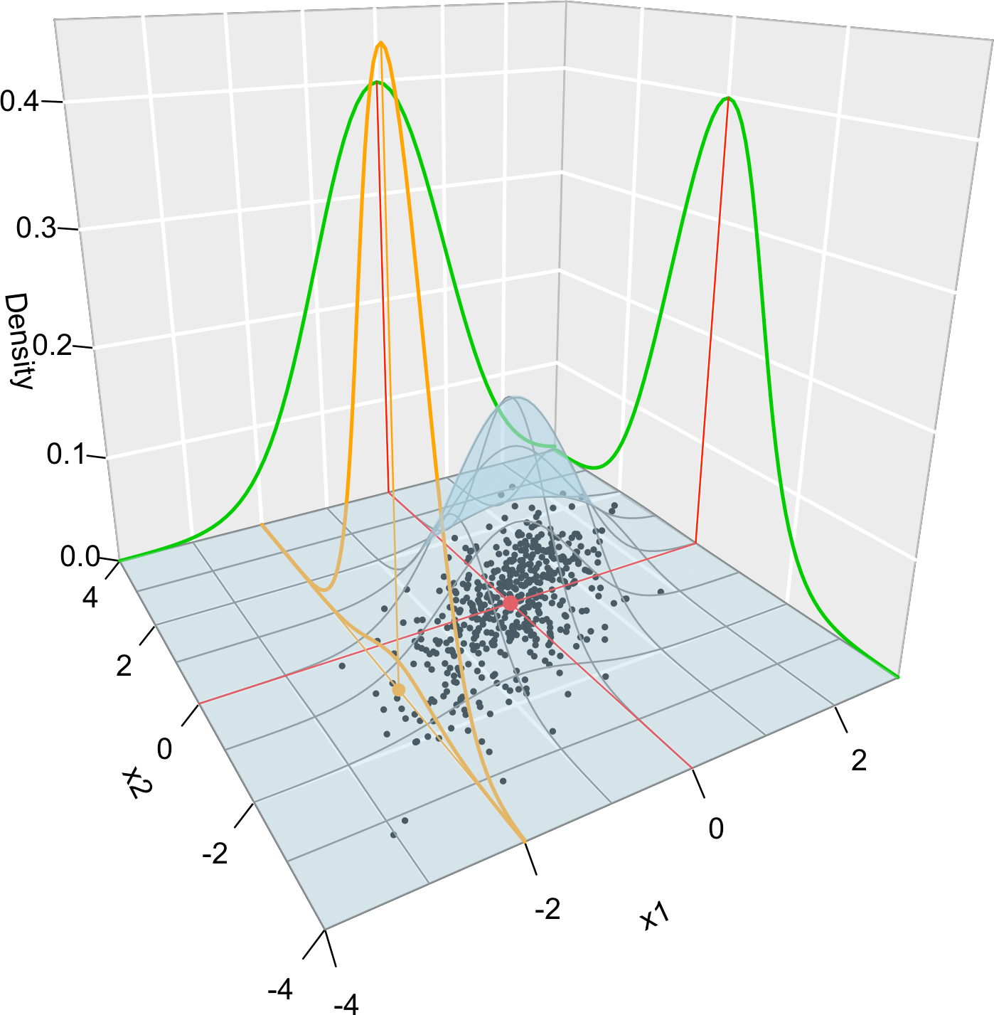
$Visualization of the joint pdf (in blue), marginal pdfs (green), conditional pdf of $X_2 \mid X_1=x_1$ (orange), expectation (red point), and conditional expectation $\mathbb{E}\lbrack X_2 \mid X_1=x_1 \rbrack$ (orange point) of a $2$-dimensional normal. The conditioning point of $X_1$ is $x_1=-2.$ Note the different scales of the densities, as they have to integrate one over different supports. Note how the conditional density (upper orange curve) is not the joint pdf $f(x_1,x_2)$ (lower orange curve) with $x_1=-2$ but a rescaling of this curve by $\frac{1}{f_{X_1}(x_1)}.$ The parameters of the $2$-dimensional normal are $\mu_1=\mu_2=0,$ $\sigma_1=\sigma_2=1$ and $\rho=0.75.$ $500$ observations sampled from the distribution are shown in black.$

Figure 1.4: Visualization of the joint pdf (in blue), marginal pdfs (green), conditional pdf of $X_2 \mid X_1=x_1$ (orange), expectation (red point), and conditional expectation $\mathbb{E}\lbrack X_2 \mid X_1=x_1 \rbrack$ (orange point) of a $2$-dimensional normal. The conditioning point of $X_1$ is $x_1=-2.$ Note the different scales of the densities, as they have to integrate one over different supports. Note how the conditional density (upper orange curve) is not the joint pdf $f(x_1,x_2)$ (lower orange curve) with $x_1=-2$ but a rescaling of this curve by $\frac{1}{f_{X_1}(x_1)}.$ The parameters of the $2$-dimensional normal are $\mu_1=\mu_2=0,$ $\sigma_1=\sigma_2=1$ and $\rho=0.75.$ $500$ observations sampled from the distribution are shown in black.

Finally, in the predictive models we will consider an independent and identically distributed (iid) sample of the response and the predictors. We use the following notation: $Y_i$ is the $i$-th observation of the response $Y$ and $X_{ij}$ represents the $i$-th observation of the $j$-th predictor $X_j.$ Thus we will deal with samples of the form $\{(X_{i1},\ldots,X_{ip},Y_i)\}_{i=1}^n.$

The relation is encoded in average by means of the conditional expectation.↩︎
That can be regarded as “structures for $m$”.↩︎
This is an alternative useful view of $\varepsilon$: the aggregation of the effects that we cannot account for predicting $Y.$↩︎
Note we use the information that $m$ has to be of a particular form (in this case quadratic) which is an unrealistic situation for other data applications.↩︎
Not only that but they are neatly interpretable.↩︎
Particularly, it usually happens that the inference based on erroneous assumptions underestimates variability, as the assumptions tend to ensure that the information of the sample is maximal for estimating the model at hand. Thus, inference based on erroneous assumptions results in a false sense of confidence: a larger error is made in reality than the one the model theory states.↩︎
Three datasets if we are fitting hyperparameters or tuning parameters in our model: the training dataset for estimating the model parameters; the validation dataset for estimating the hyper-parameters; and the testing dataset for evaluating the final performance of the fitted model.↩︎
Respectively, $F(x)=\int_{-\infty}^xf(t)\,\mathrm{d}t.$↩︎
The precise mathematical meaning of “$\mathrm{d}F_X(x)$” is the Riemann–Stieltjes integral.↩︎
Understood as the probability that $(X_1\leq x_1)$ and $\ldots$ and $(X_p\leq x_p).$↩︎
Recall that the $X$-part of $\mathbb{E}[Y \mid X]$ is random. However, $\mathbb{E}[Y \mid X=x]$ is deterministic.↩︎
If $\mu=0$ and $\sigma=1$ (standard normal), then the pdf and cdf are simply denoted by $\phi$ and $\Phi,$ without extra parameters.↩︎

Welcome

2 Linear models I: multiple linear model