3 Linear models II: model selection, extensions, and diagnostics

Given the response \(Y\) and the predictors \(X_1,\ldots,X_p,\) many linear models can be built for predicting and explaining \(Y.\) In this chapter we will see how to address the problem of selecting the best subset of predictors \(X_1,\ldots,X_p\) for explaining \(Y.\) Among others, we will also see how to extend the linear model to account for nonlinear relations between \(Y\) and \(X_1,\ldots,X_p,\) how to check whether the assumptions of the model are realistic in practice, and how to incorporate dimension reduction within linear regression.

3.1 Case study: Housing values in Boston

This case study is motivated by Harrison and Rubinfeld (1978), who proposed a hedonic model⁵¹ for determining the willingness of house buyers to pay for clean air. The study of Harrison and Rubinfeld (1978) employed data from the Boston metropolitan area, containing 560 suburbs and 14 variables. The Boston dataset is available through the file Boston.xlsx and through the dataset MASS::Boston.

The description of the related variables can be found in ?Boston and Harrison and Rubinfeld (1978),⁵² but we summarize here the most important ones as they appear in Boston. They are aggregated into five categories:

• Dependent variable: medv, the median value of owner-occupied homes (in thousands of dollars).
• Structural variables indicating the house characteristics: rm (average number of rooms “in owner units”) and age (proportion of owner-occupied units built prior to 1940).
• Neighborhood variables: crim (crime rate), zn (proportion of residential areas), indus (proportion of non-retail business area), chas (whether there is river limitation), tax (cost of public services in each community), ptratio (pupil-teacher ratio), black (variable \(1000(B - 0.63)^2,\) where \(B\) is the proportion of black population – low and high values of \(B\) increase housing prices) and lstat (percent of lower status of the population).
• Accessibility variables: dis (distances to five employment centers) and rad (accessibility to radial highways – larger index denotes better accessibility).
• Air pollution variable: nox, the annual concentration of nitrogen oxide (in parts per ten million).

We begin by importing the data:

# Read data
Boston <- readxl::read_excel(path = "Boston.xlsx", sheet = 1, col_names = TRUE)

# # Alternatively
# data(Boston, package = "MASS")

A quick summary of the data is shown below:

summary(Boston)
##       crim                zn             indus            chas              nox               rm       
##  Min.   : 0.00632   Min.   :  0.00   Min.   : 0.46   Min.   :0.00000   Min.   :0.3850   Min.   :3.561  
##  1st Qu.: 0.08205   1st Qu.:  0.00   1st Qu.: 5.19   1st Qu.:0.00000   1st Qu.:0.4490   1st Qu.:5.886  
##  Median : 0.25651   Median :  0.00   Median : 9.69   Median :0.00000   Median :0.5380   Median :6.208  
##  Mean   : 3.61352   Mean   : 11.36   Mean   :11.14   Mean   :0.06917   Mean   :0.5547   Mean   :6.285  
##  3rd Qu.: 3.67708   3rd Qu.: 12.50   3rd Qu.:18.10   3rd Qu.:0.00000   3rd Qu.:0.6240   3rd Qu.:6.623  
##  Max.   :88.97620   Max.   :100.00   Max.   :27.74   Max.   :1.00000   Max.   :0.8710   Max.   :8.780  
##       age              dis              rad              tax           ptratio          black            lstat      
##  Min.   :  2.90   Min.   : 1.130   Min.   : 1.000   Min.   :187.0   Min.   :12.60   Min.   :  0.32   Min.   : 1.73  
##  1st Qu.: 45.02   1st Qu.: 2.100   1st Qu.: 4.000   1st Qu.:279.0   1st Qu.:17.40   1st Qu.:375.38   1st Qu.: 6.95  
##  Median : 77.50   Median : 3.207   Median : 5.000   Median :330.0   Median :19.05   Median :391.44   Median :11.36  
##  Mean   : 68.57   Mean   : 3.795   Mean   : 9.549   Mean   :408.2   Mean   :18.46   Mean   :356.67   Mean   :12.65  
##  3rd Qu.: 94.08   3rd Qu.: 5.188   3rd Qu.:24.000   3rd Qu.:666.0   3rd Qu.:20.20   3rd Qu.:396.23   3rd Qu.:16.95  
##  Max.   :100.00   Max.   :12.127   Max.   :24.000   Max.   :711.0   Max.   :22.00   Max.   :396.90   Max.   :37.97  
##       medv      
##  Min.   : 5.00  
##  1st Qu.:17.02  
##  Median :21.20  
##  Mean   :22.53  
##  3rd Qu.:25.00  
##  Max.   :50.00

The two goals of this case study are:

• Q1. Quantify the influence of the predictor variables in the housing prices.
• Q2. Obtain the “best possible” model for decomposing the housing prices and interpret it.

We begin by making an exploratory analysis of the data with a matrix scatterplot. Since the number of variables is high, we opt to plot only five variables: crim, dis, medv, nox, and rm. Each of them represents the five categories in which variables were classified.

car::scatterplotMatrix(~ crim + dis + medv + nox + rm, regLine = list(col = 2),
                       col = 1, smooth = list(col.smooth = 4, col.spread = 4),
                       data = Boston)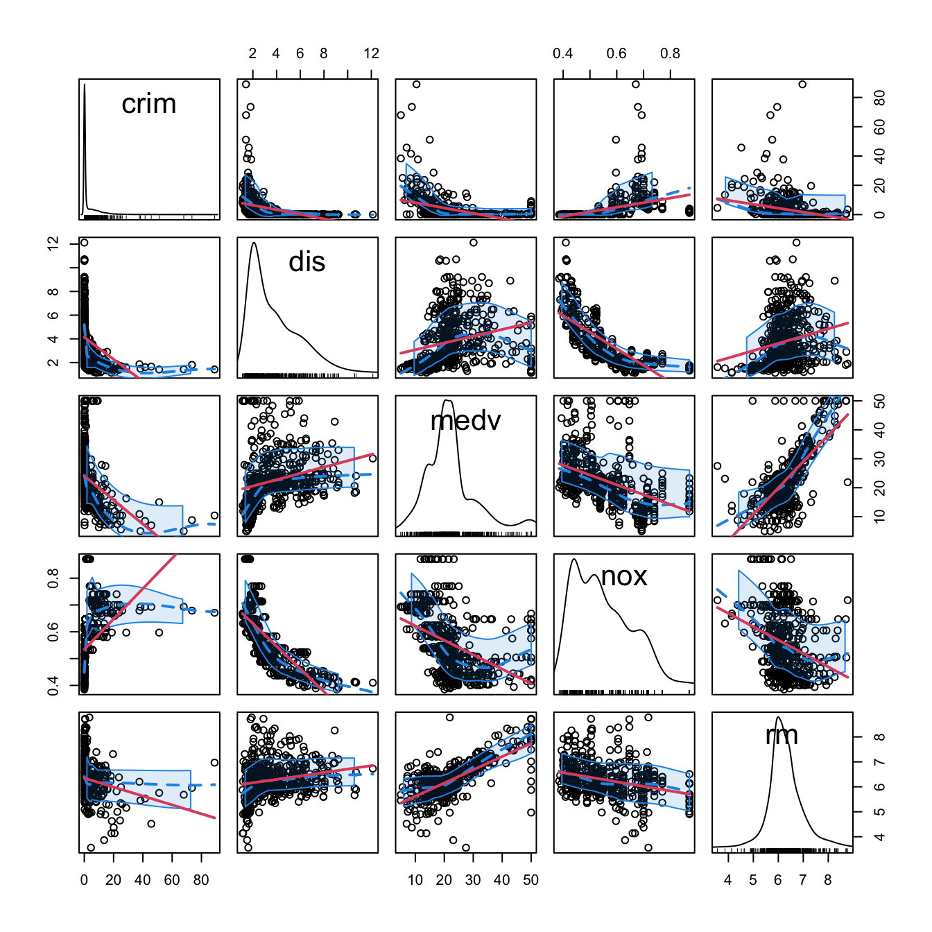

Figure 3.1: Scatterplot matrix for crim, dis, medv, nox, and rm from the Boston dataset. The diagonal panels show an estimate of the unknown pdf of each variable (see Section 6.1.2). The red and blue lines are linear and nonparametric (see Section 6.2) estimates of the regression functions for pairwise relations.

Note the peculiar distribution of crim, very concentrated at zero, and the asymmetry in medv, with a second mode associated with the most expensive properties. Inspecting the individual panels, it is clear that some nonlinearity exists in the data and that some predictors are going to be more important than others (and recall that we have plotted just a subset of all the predictors).

3.2 Model selection

In Chapter 2 we briefly saw that the inclusion of more predictors is not for free: there is a price to pay in terms of more variability in the coefficients estimates, harder interpretation, and possible inclusion of highly-dependent predictors. Indeed, there is a maximum number of predictors \(p\) that can be considered in a linear model for a sample size \(n\): \[\begin{align*} p\leq n-2. \end{align*}\] Equivalently, there is a minimum sample size \(n\) required for fitting a model with \(p\) predictors: \(n\geq p + 2.\)

The interpretation of this fact is simple if we think about the geometry for \(p=1\) and \(p=2\):

• If \(p=1,\) we need at least \(n=2\) points to uniquely fit a line. However, this line gives no information on the vertical variation about it, hence \(\sigma^2\) cannot be estimated.⁵³ Therefore, we need at least \(n=3\) points, that is, \(n\geq p + 2=3.\)
• If \(p=2,\) we need at least \(n=3\) points to uniquely fit a plane. But again this plane gives no information on the variation of the data about it and hence \(\sigma^2\) cannot be estimated. Therefore, we need \(n\geq p + 2=4.\)

Another interpretation is the following:

The fitting of a linear model with \(p\) predictors involves the estimation of \(p+2\) parameters \((\boldsymbol{\beta},\sigma^2)\) from \(n\) data points. The closer \(p+2\) and \(n\) are, the more variable the estimates \((\hat{\boldsymbol{\beta}},\hat\sigma^2)\) will be, since less information is available for estimating each one. In the limit case \(n=p+2,\) each sample point determines a parameter estimate.

In the above discussion the degenerate case \(p=n-1\) was excluded, as it gives a perfect and useless fit for which \(\hat\sigma^2\) is not defined. However, \(\hat{\boldsymbol{\beta}}\) is actually computable if \(p=n-1.\) The output of the next chunk of code clarifies the distinction between \(p=n-1\) and \(p=n-2.\)

# Data: n observations and p = n - 1 predictors
set.seed(123456)
n <- 5
p <- n - 1
df <- data.frame(y = rnorm(n), x = matrix(rnorm(n * p), nrow = n, ncol = p))

# Case p = n - 1 = 4: beta can be estimated, but sigma^2 cannot (hence, no
# inference can be performed since it requires the estimated sigma^2)
summary(lm(y ~ ., data = df))

# Case p = n - 2 = 3: both beta and sigma^2 can be estimated (hence, inference
# can be performed)
summary(lm(y ~ . - x.1, data = df))

The degrees of freedom \(n-p-1\) quantify the increase in the variability of \((\hat{\boldsymbol{\beta}},\hat\sigma^2)\) when \(p\) approaches \(n-2.\) For example:

• \(t_{n-p-1;\alpha/2}\) appears in (2.16) and influences the length of the CIs for \(\beta_j,\) see (2.17). It also influences the length of the CIs for the prediction. As Figure 3.2 shows, when the degrees of freedom decrease, \(t_{n-p-1;\alpha/2}\) increases, thus the intervals widen.
• \(\hat\sigma^2=\frac{1}{n-p-1}\sum_{i=1}^n\hat\varepsilon_i^2\) influences the \(R^2\) and \(R^2_\text{Adj}.\) If no relevant variables are added to the model then \(\sum_{i=1}^n\hat\varepsilon_i^2\) will not change substantially. However, the factor \(\frac{1}{n-p-1}\) will increase as \(p\) augments, inflating \(\hat\sigma^2\) and its variance. This is exactly what happened in Figure 2.19.

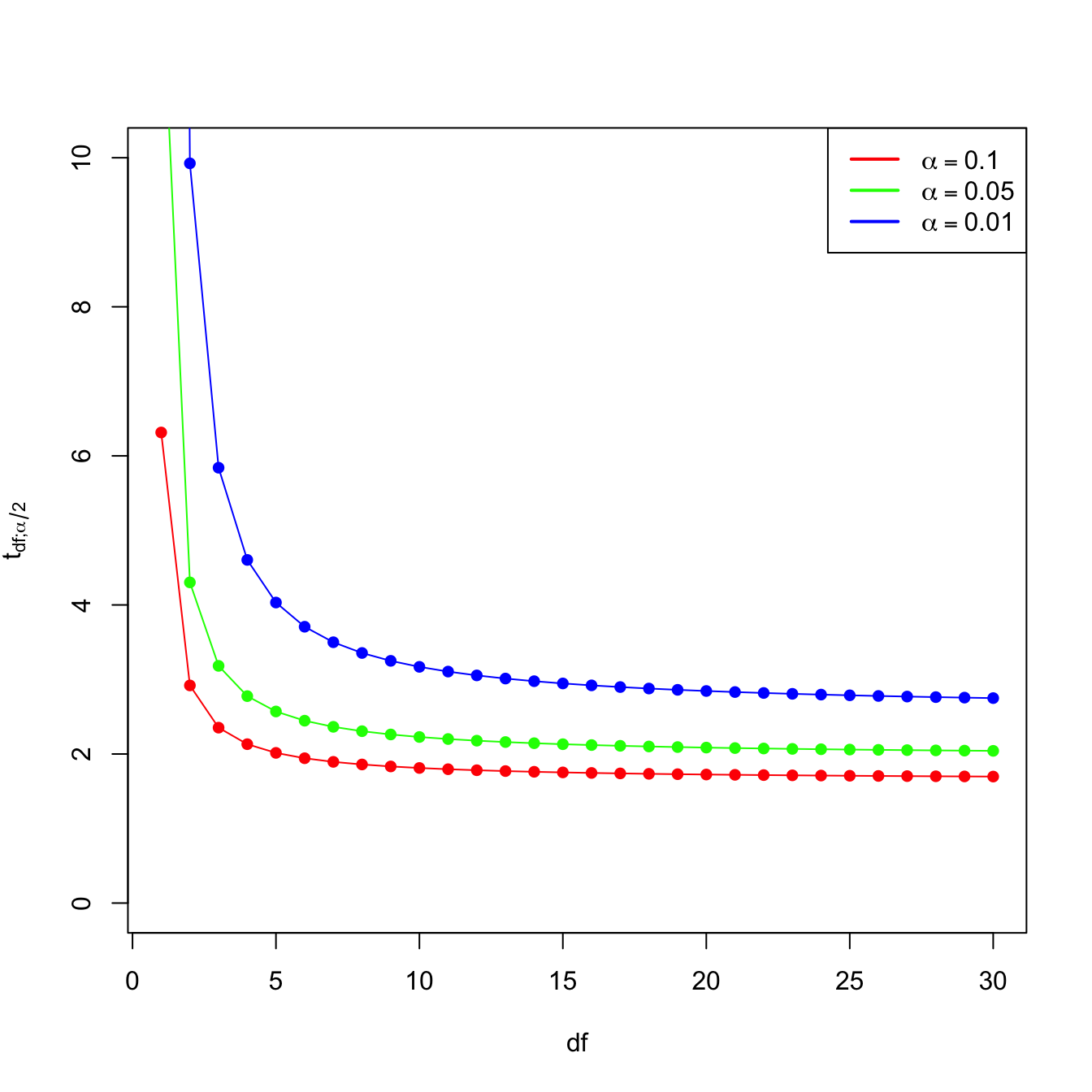
Figure 3.2: Effect of \(\text{df}=n-p-1\) in \(t_{\text{df};\alpha/2}\) for \(\alpha=0.10,0.05,0.01.\)

Now that we have shed more light on the problem of having an excess of predictors, we turn the focus on selecting the most adequate predictors for a multiple regression model. This is a challenging task without a unique solution, and what is worse, without a method that is guaranteed to work in all the cases. However, there is a well-established procedure that usually gives good results: the stepwise model selection. Its principle is to sequentially compare multiple linear regression models with different predictors,⁵⁴ improving iteratively a performance measure through a greedy search.

Stepwise model selection typically uses as measure of performance an information criterion. An information criterion balances the fitness of a model with the number of predictors employed. Hence, it determines objectively the best model as the one that minimizes the considered information criterion. Two common criteria are the Bayesian Information Criterion (BIC) and the Akaike Information Criterion (AIC). Both are based on balancing the model fitness and its complexity:

\[\begin{align} \text{BIC}(\text{model}) = \underbrace{-2\ell(\text{model})}_{\text{Model fitness}} + \underbrace{\text{npar(model)}\times\log(n)}_{\text{Complexity}}, \tag{3.1} \end{align}\]

where \(\ell(\text{model})\) is the log-likelihood of the model (how well the model fits the data) and \(\text{npar(model)}\) is the number of parameters considered in the model (how complex the model is). In the case of a multiple linear regression model with \(p\) predictors, \(\text{npar(model)}=p+2.\) The AIC replaces the \(\log(n)\) factor by a \(2\) in (3.1) so, compared with the BIC, it penalizes less the more complex models.⁵⁵ This is one of the reasons why BIC is preferred by some practitioners for performing model comparison⁵⁶

The BIC and AIC can be computed through the functions BIC and AIC. They take a model as the input.

# Two models with different predictors
mod1 <- lm(medv ~ age + crim, data = Boston)
mod2 <- lm(medv ~ age + crim + lstat, data = Boston)

# BICs
BIC(mod1)
## [1] 3581.893
BIC(mod2) # Smaller -> better
## [1] 3300.841

# AICs
AIC(mod1)
## [1] 3564.987
AIC(mod2) # Smaller -> better
## [1] 3279.708

# Check the summaries
summary(mod1)
## 
## Call:
## lm(formula = medv ~ age + crim, data = Boston)
## 
## Residuals:
##     Min      1Q  Median      3Q     Max 
## -13.940  -4.991  -2.420   2.110  32.033 
## 
## Coefficients:
##             Estimate Std. Error t value Pr(>|t|)    
## (Intercept) 29.80067    0.97078  30.698  < 2e-16 ***
## age         -0.08955    0.01378  -6.499 1.95e-10 ***
## crim        -0.31182    0.04510  -6.914 1.43e-11 ***
## ---
## Signif. codes:  0 '***' 0.001 '**' 0.01 '*' 0.05 '.' 0.1 ' ' 1
## 
## Residual standard error: 8.157 on 503 degrees of freedom
## Multiple R-squared:  0.2166, Adjusted R-squared:  0.2134 
## F-statistic: 69.52 on 2 and 503 DF,  p-value: < 2.2e-16
summary(mod2)
## 
## Call:
## lm(formula = medv ~ age + crim + lstat, data = Boston)
## 
## Residuals:
##     Min      1Q  Median      3Q     Max 
## -16.133  -3.848  -1.380   1.970  23.644 
## 
## Coefficients:
##             Estimate Std. Error t value Pr(>|t|)    
## (Intercept) 32.82804    0.74774  43.903  < 2e-16 ***
## age          0.03765    0.01225   3.074  0.00223 ** 
## crim        -0.08262    0.03594  -2.299  0.02193 *  
## lstat       -0.99409    0.05075 -19.587  < 2e-16 ***
## ---
## Signif. codes:  0 '***' 0.001 '**' 0.01 '*' 0.05 '.' 0.1 ' ' 1
## 
## Residual standard error: 6.147 on 502 degrees of freedom
## Multiple R-squared:  0.5559, Adjusted R-squared:  0.5533 
## F-statistic: 209.5 on 3 and 502 DF,  p-value: < 2.2e-16

Let’s go back to the selection of predictors. If we have \(p\) predictors, a naive procedure would be to check all the possible models that can be constructed with them and then select the best one in terms of BIC/AIC. This exhaustive search is the so-called best subset selection – its application to be seen in Section 4.4. The problem is that there are \(2^p\) possible models to inspect!⁵⁷ Fortunately, the MASS::stepAIC function helps us navigating this ocean of models by implementing stepwise model selection. Stepwise selection will iteratively add predictors that decrease an information criterion and/or remove those that increase it, depending on the mode of stepwise search that is performed.

stepAIC takes as input an initial model to be improved and has several variants. Let’s see first how it works in its default mode using the already studied wine dataset.

# Load data -- notice that "Year" is also included
wine <- read.csv(file = "wine.csv", header = TRUE)

We use as initial model the one featuring all the available predictors. The argument k of stepAIC stands for the factor post-multiplying \(\text{npar(model)}\) in (3.1). It defaults to \(2,\) which gives the AIC. If we set it to k = log(n), the function considers the BIC.

# Full model
mod <- lm(Price ~ ., data = wine)

# With AIC
modAIC <- MASS::stepAIC(mod, k = 2)
## Start:  AIC=-61.07
## Price ~ Year + WinterRain + AGST + HarvestRain + Age + FrancePop
## 
## 
## Step:  AIC=-61.07
## Price ~ Year + WinterRain + AGST + HarvestRain + FrancePop
## 
##               Df Sum of Sq    RSS     AIC
## - FrancePop    1    0.0026 1.8058 -63.031
## - Year         1    0.0048 1.8080 -62.998
## <none>                     1.8032 -61.070
## - WinterRain   1    0.4585 2.2617 -56.952
## - HarvestRain  1    1.8063 3.6095 -44.331
## - AGST         1    3.3756 5.1788 -34.584
## 
## Step:  AIC=-63.03
## Price ~ Year + WinterRain + AGST + HarvestRain
## 
##               Df Sum of Sq    RSS     AIC
## <none>                     1.8058 -63.031
## - WinterRain   1    0.4809 2.2867 -58.656
## - Year         1    0.9089 2.7147 -54.023
## - HarvestRain  1    1.8760 3.6818 -45.796
## - AGST         1    3.4428 5.2486 -36.222

# The result is an lm object
summary(modAIC)
## 
## Call:
## lm(formula = Price ~ Year + WinterRain + AGST + HarvestRain, 
##     data = wine)
## 
## Residuals:
##      Min       1Q   Median       3Q      Max 
## -0.46024 -0.23862  0.01347  0.18601  0.53443 
## 
## Coefficients:
##               Estimate Std. Error t value Pr(>|t|)    
## (Intercept) 43.6390418 14.6939240   2.970  0.00707 ** 
## Year        -0.0238480  0.0071667  -3.328  0.00305 ** 
## WinterRain   0.0011667  0.0004820   2.420  0.02421 *  
## AGST         0.6163916  0.0951747   6.476 1.63e-06 ***
## HarvestRain -0.0038606  0.0008075  -4.781 8.97e-05 ***
## ---
## Signif. codes:  0 '***' 0.001 '**' 0.01 '*' 0.05 '.' 0.1 ' ' 1
## 
## Residual standard error: 0.2865 on 22 degrees of freedom
## Multiple R-squared:  0.8275, Adjusted R-squared:  0.7962 
## F-statistic: 26.39 on 4 and 22 DF,  p-value: 4.057e-08

# With BIC
modBIC <- MASS::stepAIC(mod, k = log(nrow(wine)))
## Start:  AIC=-53.29
## Price ~ Year + WinterRain + AGST + HarvestRain + Age + FrancePop
## 
## 
## Step:  AIC=-53.29
## Price ~ Year + WinterRain + AGST + HarvestRain + FrancePop
## 
##               Df Sum of Sq    RSS     AIC
## - FrancePop    1    0.0026 1.8058 -56.551
## - Year         1    0.0048 1.8080 -56.519
## <none>                     1.8032 -53.295
## - WinterRain   1    0.4585 2.2617 -50.473
## - HarvestRain  1    1.8063 3.6095 -37.852
## - AGST         1    3.3756 5.1788 -28.105
## 
## Step:  AIC=-56.55
## Price ~ Year + WinterRain + AGST + HarvestRain
## 
##               Df Sum of Sq    RSS     AIC
## <none>                     1.8058 -56.551
## - WinterRain   1    0.4809 2.2867 -53.473
## - Year         1    0.9089 2.7147 -48.840
## - HarvestRain  1    1.8760 3.6818 -40.612
## - AGST         1    3.4428 5.2486 -31.039

An explanation of what stepAIC did for modBIC:

• At each step, stepAIC displayed information about the current value of the information criterion. For example, the BIC at the first step was Step: AIC=-53.29 and then it improved to Step: AIC=-56.55 in the second step.⁵⁸
• The next model to move on was decided by exploring the information criteria of the different models resulting from adding or removing a predictor (depending on the direction argument, explained later). For example, in the first step the model arising from removing⁵⁹ FrancePop had a BIC equal to -56.551.
• The stepwise regression proceeded then by removing FrancePop, as it gave the lowest BIC. When repeating the previous exploration, it was found that removing <none> predictors was the best possible action.

The selected models modBIC and modAIC are equivalent to the modWine2 we selected in Section 2.7.3 as the best model. This is a simple illustration that the model selected by stepAIC is often a good starting point for further additions or deletions of predictors.

The direction argument of stepAIC controls the mode of the stepwise model search:

• "backward": removes predictors sequentially from the given model. It produces a sequence of models of decreasing complexity until attaining the optimal one.
• "forward": adds predictors sequentially to the given model, using the available ones in the data argument of lm. It produces a sequence of models of increasing complexity until attaining the optimal one.
• "both" (default): a forward-backward search that, at each step, decides whether to include or exclude a predictor. Differently from the previous modes, a predictor that was excluded/included previously can be later included/excluded.

The next chunk of code clearly explains how to exploit the direction argument, and other options of stepAIC, with a modified version of the wine dataset. An important warning is that in order to use direction = "forward" or direction = "both", scope needs to be properly defined. The practical advice to model selection is to run⁶⁰ several of these three search modes and retain the model with minimum BIC/AIC, being specially careful with the scope argument.

# Add an irrelevant predictor to the wine dataset
set.seed(123456)
wineNoise <- wine
n <- nrow(wineNoise)
wineNoise$noisePredictor <- rnorm(n)

# Backward selection: removes predictors sequentially from the given model

# Starting from the model with all the predictors
modAll <- lm(formula = Price ~ ., data = wineNoise)
MASS::stepAIC(modAll, direction = "backward", k = log(n))
## Start:  AIC=-50.13
## Price ~ Year + WinterRain + AGST + HarvestRain + Age + FrancePop + 
##     noisePredictor
## 
## 
## Step:  AIC=-50.13
## Price ~ Year + WinterRain + AGST + HarvestRain + FrancePop + 
##     noisePredictor
## 
##                  Df Sum of Sq    RSS     AIC
## - FrancePop       1    0.0036 1.7977 -53.376
## - Year            1    0.0038 1.7979 -53.374
## - noisePredictor  1    0.0090 1.8032 -53.295
## <none>                        1.7941 -50.135
## - WinterRain      1    0.4598 2.2539 -47.271
## - HarvestRain     1    1.7666 3.5607 -34.923
## - AGST            1    3.3658 5.1599 -24.908
## 
## Step:  AIC=-53.38
## Price ~ Year + WinterRain + AGST + HarvestRain + noisePredictor
## 
##                  Df Sum of Sq    RSS     AIC
## - noisePredictor  1    0.0081 1.8058 -56.551
## <none>                        1.7977 -53.376
## - WinterRain      1    0.4771 2.2748 -50.317
## - Year            1    0.9162 2.7139 -45.552
## - HarvestRain     1    1.8449 3.6426 -37.606
## - AGST            1    3.4234 5.2212 -27.885
## 
## Step:  AIC=-56.55
## Price ~ Year + WinterRain + AGST + HarvestRain
## 
##               Df Sum of Sq    RSS     AIC
## <none>                     1.8058 -56.551
## - WinterRain   1    0.4809 2.2867 -53.473
## - Year         1    0.9089 2.7147 -48.840
## - HarvestRain  1    1.8760 3.6818 -40.612
## - AGST         1    3.4428 5.2486 -31.039
## 
## Call:
## lm(formula = Price ~ Year + WinterRain + AGST + HarvestRain, 
##     data = wineNoise)
## 
## Coefficients:
## (Intercept)         Year   WinterRain         AGST  HarvestRain  
##   43.639042    -0.023848     0.001167     0.616392    -0.003861

# Starting from an intermediate model
modInter <- lm(formula = Price ~ noisePredictor + Year + AGST, data = wineNoise)
MASS::stepAIC(modInter, direction = "backward", k = log(n))
## Start:  AIC=-32.38
## Price ~ noisePredictor + Year + AGST
## 
##                  Df Sum of Sq    RSS     AIC
## - noisePredictor  1    0.0146 5.0082 -35.601
## <none>                        4.9936 -32.384
## - Year            1    0.7522 5.7459 -31.891
## - AGST            1    3.2211 8.2147 -22.240
## 
## Step:  AIC=-35.6
## Price ~ Year + AGST
## 
##        Df Sum of Sq    RSS     AIC
## <none>              5.0082 -35.601
## - Year  1    0.7966 5.8049 -34.911
## - AGST  1    3.2426 8.2509 -25.417
## 
## Call:
## lm(formula = Price ~ Year + AGST, data = wineNoise)
## 
## Coefficients:
## (Intercept)         Year         AGST  
##    41.49441     -0.02221      0.56067
# Recall that other predictors not included in modInter are not explored
# during the search (so the relevant predictor HarvestRain is not added)

# Forward selection: adds predictors sequentially from the given model

# Starting from the model with no predictors, only intercept (denoted as ~ 1)
modZero <- lm(formula = Price ~ 1, data = wineNoise)
MASS::stepAIC(modZero, direction = "forward",
              scope = list(lower = modZero, upper = modAll), k = log(n))
## Start:  AIC=-22.28
## Price ~ 1
## 
##                  Df Sum of Sq     RSS     AIC
## + AGST            1    4.6655  5.8049 -34.911
## + HarvestRain     1    2.6933  7.7770 -27.014
## + FrancePop       1    2.4231  8.0472 -26.092
## + Year            1    2.2195  8.2509 -25.417
## + Age             1    2.2195  8.2509 -25.417
## <none>                        10.4703 -22.281
## + WinterRain      1    0.1905 10.2798 -19.481
## + noisePredictor  1    0.1761 10.2942 -19.443
## 
## Step:  AIC=-34.91
## Price ~ AGST
## 
##                  Df Sum of Sq    RSS     AIC
## + HarvestRain     1   2.50659 3.2983 -46.878
## + WinterRain      1   1.42392 4.3809 -39.214
## + FrancePop       1   0.90263 4.9022 -36.178
## + Year            1   0.79662 5.0082 -35.601
## + Age             1   0.79662 5.0082 -35.601
## <none>                        5.8049 -34.911
## + noisePredictor  1   0.05900 5.7459 -31.891
## 
## Step:  AIC=-46.88
## Price ~ AGST + HarvestRain
## 
##                  Df Sum of Sq    RSS     AIC
## + FrancePop       1   1.03572 2.2625 -53.759
## + Year            1   1.01159 2.2867 -53.473
## + Age             1   1.01159 2.2867 -53.473
## + WinterRain      1   0.58356 2.7147 -48.840
## <none>                        3.2983 -46.878
## + noisePredictor  1   0.06084 3.2374 -44.085
## 
## Step:  AIC=-53.76
## Price ~ AGST + HarvestRain + FrancePop
## 
##                  Df Sum of Sq    RSS     AIC
## + WinterRain      1   0.45456 1.8080 -56.519
## <none>                        2.2625 -53.759
## + noisePredictor  1   0.00829 2.2542 -50.562
## + Year            1   0.00085 2.2617 -50.473
## + Age             1   0.00085 2.2617 -50.473
## 
## Step:  AIC=-56.52
## Price ~ AGST + HarvestRain + FrancePop + WinterRain
## 
##                  Df Sum of Sq    RSS     AIC
## <none>                        1.8080 -56.519
## + noisePredictor  1 0.0100635 1.7979 -53.374
## + Year            1 0.0048039 1.8032 -53.295
## + Age             1 0.0048039 1.8032 -53.295
## 
## Call:
## lm(formula = Price ~ AGST + HarvestRain + FrancePop + WinterRain, 
##     data = wineNoise)
## 
## Coefficients:
## (Intercept)         AGST  HarvestRain    FrancePop   WinterRain  
##  -5.945e-01    6.127e-01   -3.804e-03   -5.189e-05    1.136e-03
# It is very important to set the scope argument adequately when doing forward
# search! In the scope you have to define the "minimum" (lower) and "maximum"
# (upper) models that contain the set of explorable models. If not provided,
# the maximum model will be taken as the passed starting model (in this case
# modZero) and stepAIC will not do any search

# Starting from an intermediate model
MASS::stepAIC(modInter, direction = "forward",
              scope = list(lower = modZero, upper = modAll), k = log(n))
## Start:  AIC=-32.38
## Price ~ noisePredictor + Year + AGST
## 
##               Df Sum of Sq    RSS     AIC
## + HarvestRain  1   2.71878 2.2748 -50.317
## + WinterRain   1   1.35102 3.6426 -37.606
## <none>                     4.9936 -32.384
## + FrancePop    1   0.24004 4.7536 -30.418
## 
## Step:  AIC=-50.32
## Price ~ noisePredictor + Year + AGST + HarvestRain
## 
##              Df Sum of Sq    RSS     AIC
## + WinterRain  1   0.47710 1.7977 -53.376
## <none>                    2.2748 -50.317
## + FrancePop   1   0.02094 2.2539 -47.271
## 
## Step:  AIC=-53.38
## Price ~ noisePredictor + Year + AGST + HarvestRain + WinterRain
## 
##             Df Sum of Sq    RSS     AIC
## <none>                   1.7977 -53.376
## + FrancePop  1 0.0036037 1.7941 -50.135
## 
## Call:
## lm(formula = Price ~ noisePredictor + Year + AGST + HarvestRain + 
##     WinterRain, data = wineNoise)
## 
## Coefficients:
##    (Intercept)  noisePredictor            Year            AGST     HarvestRain      WinterRain  
##      44.096639       -0.019617       -0.024126        0.620522       -0.003840        0.001211
# Recall that predictors included in modInter are not dropped during the
# search (so the irrelevant noisePredictor is kept)

# Both selection: useful if starting from an intermediate model

# Removes the problems associated with "backward" and "forward" searches done
# from intermediate models
MASS::stepAIC(modInter, direction = "both",
              scope = list(lower = modZero, upper = modAll), k = log(n))
## Start:  AIC=-32.38
## Price ~ noisePredictor + Year + AGST
## 
##                  Df Sum of Sq    RSS     AIC
## + HarvestRain     1    2.7188 2.2748 -50.317
## + WinterRain      1    1.3510 3.6426 -37.606
## - noisePredictor  1    0.0146 5.0082 -35.601
## <none>                        4.9936 -32.384
## - Year            1    0.7522 5.7459 -31.891
## + FrancePop       1    0.2400 4.7536 -30.418
## - AGST            1    3.2211 8.2147 -22.240
## 
## Step:  AIC=-50.32
## Price ~ noisePredictor + Year + AGST + HarvestRain
## 
##                  Df Sum of Sq    RSS     AIC
## - noisePredictor  1   0.01182 2.2867 -53.473
## + WinterRain      1   0.47710 1.7977 -53.376
## <none>                        2.2748 -50.317
## + FrancePop       1   0.02094 2.2539 -47.271
## - Year            1   0.96258 3.2374 -44.085
## - HarvestRain     1   2.71878 4.9936 -32.384
## - AGST            1   2.94647 5.2213 -31.180
## 
## Step:  AIC=-53.47
## Price ~ Year + AGST + HarvestRain
## 
##                  Df Sum of Sq    RSS     AIC
## + WinterRain      1   0.48087 1.8058 -56.551
## <none>                        2.2867 -53.473
## + FrancePop       1   0.02497 2.2617 -50.473
## + noisePredictor  1   0.01182 2.2748 -50.317
## - Year            1   1.01159 3.2983 -46.878
## - HarvestRain     1   2.72157 5.0082 -35.601
## - AGST            1   2.96500 5.2517 -34.319
## 
## Step:  AIC=-56.55
## Price ~ Year + AGST + HarvestRain + WinterRain
## 
##                  Df Sum of Sq    RSS     AIC
## <none>                        1.8058 -56.551
## - WinterRain      1    0.4809 2.2867 -53.473
## + noisePredictor  1    0.0081 1.7977 -53.376
## + FrancePop       1    0.0026 1.8032 -53.295
## - Year            1    0.9089 2.7147 -48.840
## - HarvestRain     1    1.8760 3.6818 -40.612
## - AGST            1    3.4428 5.2486 -31.039
## 
## Call:
## lm(formula = Price ~ Year + AGST + HarvestRain + WinterRain, 
##     data = wineNoise)
## 
## Coefficients:
## (Intercept)         Year         AGST  HarvestRain   WinterRain  
##   43.639042    -0.023848     0.616392    -0.003861     0.001167
# It is very important as well to correctly define the scope, because "both"
# resorts to "forward" (as well as to "backward")

# Using the defaults from the full model essentially does backward selection,
# but allowing predictors that were removed to enter again at later steps
MASS::stepAIC(modAll, direction = "both", k = log(n))
## Start:  AIC=-50.13
## Price ~ Year + WinterRain + AGST + HarvestRain + Age + FrancePop + 
##     noisePredictor
## 
## 
## Step:  AIC=-50.13
## Price ~ Year + WinterRain + AGST + HarvestRain + FrancePop + 
##     noisePredictor
## 
##                  Df Sum of Sq    RSS     AIC
## - FrancePop       1    0.0036 1.7977 -53.376
## - Year            1    0.0038 1.7979 -53.374
## - noisePredictor  1    0.0090 1.8032 -53.295
## <none>                        1.7941 -50.135
## - WinterRain      1    0.4598 2.2539 -47.271
## - HarvestRain     1    1.7666 3.5607 -34.923
## - AGST            1    3.3658 5.1599 -24.908
## 
## Step:  AIC=-53.38
## Price ~ Year + WinterRain + AGST + HarvestRain + noisePredictor
## 
##                  Df Sum of Sq    RSS     AIC
## - noisePredictor  1    0.0081 1.8058 -56.551
## <none>                        1.7977 -53.376
## - WinterRain      1    0.4771 2.2748 -50.317
## + FrancePop       1    0.0036 1.7941 -50.135
## - Year            1    0.9162 2.7139 -45.552
## - HarvestRain     1    1.8449 3.6426 -37.606
## - AGST            1    3.4234 5.2212 -27.885
## 
## Step:  AIC=-56.55
## Price ~ Year + WinterRain + AGST + HarvestRain
## 
##                  Df Sum of Sq    RSS     AIC
## <none>                        1.8058 -56.551
## - WinterRain      1    0.4809 2.2867 -53.473
## + noisePredictor  1    0.0081 1.7977 -53.376
## + FrancePop       1    0.0026 1.8032 -53.295
## - Year            1    0.9089 2.7147 -48.840
## - HarvestRain     1    1.8760 3.6818 -40.612
## - AGST            1    3.4428 5.2486 -31.039
## 
## Call:
## lm(formula = Price ~ Year + WinterRain + AGST + HarvestRain, 
##     data = wineNoise)
## 
## Coefficients:
## (Intercept)         Year   WinterRain         AGST  HarvestRain  
##   43.639042    -0.023848     0.001167     0.616392    -0.003861

# Omit lengthy outputs
MASS::stepAIC(modAll, direction = "both", trace = 0,
              scope = list(lower = modZero, upper = modAll), k = log(n))
## 
## Call:
## lm(formula = Price ~ Year + WinterRain + AGST + HarvestRain, 
##     data = wineNoise)
## 
## Coefficients:
## (Intercept)         Year   WinterRain         AGST  HarvestRain  
##   43.639042    -0.023848     0.001167     0.616392    -0.003861

Exercise 3.1 Run the previous stepwise selections for the Boston dataset, with the aim of clearly understanding the different search directions. Specifically:

1. Do a "forward" stepwise fit starting from medv ~ 1.
2. Do a "forward" stepwise fit starting from medv ~ crim + lstat + age.
3. Do a "both" stepwise fit starting from medv ~ crim + lstat + age.
4. Do a "both" stepwise fit starting from medv ~ ..
5. Do a "backward" stepwise fit starting from medv ~ ..

We conclude with a couple of quirks of stepAIC to be aware of.

stepAIC assumes that no NA’s (missing values) are present in the data. It is advised to remove the missing values in the data before. Their presence might lead to errors. To do so, employ data = na.omit(dataset) in the call to lm (if your dataset is dataset). Also, see Appendix D for possible alternatives to deal with missing data.

stepAIC and friends (addterm and dropterm) compute a slightly different version of the BIC/AIC than the BIC/AIC functions. Precisely, the BIC/AIC they report come from the extractAIC function, which differs in an additive constant from the output of BIC/AIC. This is not relevant for model comparison, since shifting by a common constant the BIC/AIC does not change the lower-to-higher BIC/AIC ordering of models. However, it is important to be aware of this fact in order to do not compare directly the output of stepAIC with the one of BIC/AIC. The additive constant (included in BIC/AIC but not in extractAIC) is \(n(\log(2 \pi) + 1) + \log(n)\) for the BIC and \(n(\log(2 \pi) + 1) + 2\) for the AIC. The discrepancy arises from simplifying the computation of the BIC/AIC for linear models and from counting \(\hat\sigma^2\) as an estimated parameter.

The following chunk of code illustrates the relation of the AIC reported in stepAIC, the output of extractAIC, and the BIC/AIC reported by BIC/AIC.

# Same BICs, different scale
n <- nobs(modBIC)
extractAIC(modBIC, k = log(n))[2]
## [1] -56.55135
BIC(modBIC)
## [1] 23.36717
# Observe that MASS::stepAIC(mod, k = log(nrow(wine))) returned as final BIC
# the one given by extractAIC(), not by BIC()! But both are equivalent, they
# just differ in a constant shift

# Same AICs, different scale
extractAIC(modAIC, k = 2)[2]
## [1] -63.03053
AIC(modAIC)
## [1] 15.59215

# The additive constant: BIC() includes it but extractAIC() does not
BIC(modBIC) - extractAIC(modBIC, k = log(n))[2]
## [1] 79.91852
n * (log(2 * pi) + 1) + log(n)
## [1] 79.91852

# Same for the AIC
AIC(modAIC) - extractAIC(modAIC)[2]
## [1] 78.62268
n * (log(2 * pi) + 1) + 2
## [1] 78.62268

3.2.1 Case study application

We want to build a linear model for predicting and explaining medv. There are a good number of predictors and some of them might be of little use for predicting medv. However, there is no clear intuition of which predictors will yield better explanations of medv with the information at hand. Therefore, we can start by doing a linear model on all the predictors:

modHouse <- lm(medv ~ ., data = Boston)
summary(modHouse)
## 
## Call:
## lm(formula = medv ~ ., data = Boston)
## 
## Residuals:
##     Min      1Q  Median      3Q     Max 
## -15.595  -2.730  -0.518   1.777  26.199 
## 
## Coefficients:
##               Estimate Std. Error t value Pr(>|t|)    
## (Intercept)  3.646e+01  5.103e+00   7.144 3.28e-12 ***
## crim        -1.080e-01  3.286e-02  -3.287 0.001087 ** 
## zn           4.642e-02  1.373e-02   3.382 0.000778 ***
## indus        2.056e-02  6.150e-02   0.334 0.738288    
## chas         2.687e+00  8.616e-01   3.118 0.001925 ** 
## nox         -1.777e+01  3.820e+00  -4.651 4.25e-06 ***
## rm           3.810e+00  4.179e-01   9.116  < 2e-16 ***
## age          6.922e-04  1.321e-02   0.052 0.958229    
## dis         -1.476e+00  1.995e-01  -7.398 6.01e-13 ***
## rad          3.060e-01  6.635e-02   4.613 5.07e-06 ***
## tax         -1.233e-02  3.760e-03  -3.280 0.001112 ** 
## ptratio     -9.527e-01  1.308e-01  -7.283 1.31e-12 ***
## black        9.312e-03  2.686e-03   3.467 0.000573 ***
## lstat       -5.248e-01  5.072e-02 -10.347  < 2e-16 ***
## ---
## Signif. codes:  0 '***' 0.001 '**' 0.01 '*' 0.05 '.' 0.1 ' ' 1
## 
## Residual standard error: 4.745 on 492 degrees of freedom
## Multiple R-squared:  0.7406, Adjusted R-squared:  0.7338 
## F-statistic: 108.1 on 13 and 492 DF,  p-value: < 2.2e-16

There are a couple of non-significant variables, but so far the model has an \(R^2=0.74\) and the fitted coefficients are sensible with what would be expected. For example, crim, tax, ptratio, and nox have negative effects on medv, while rm, rad, and chas have positive effects. However, the non-significant coefficients are only adding noise to the prediction and decreasing the overall accuracy of the coefficient estimates.

Let’s polish the previous model a little bit. Instead of manually removing each non-significant variable to reduce the complexity, we employ stepAIC for performing a forward-backward search starting from the full model. This gives us a candidate best model.

# Best BIC and AIC models
modBIC <- MASS::stepAIC(modHouse, k = log(nrow(Boston)))
## Start:  AIC=1648.81
## medv ~ crim + zn + indus + chas + nox + rm + age + dis + rad + 
##     tax + ptratio + black + lstat
## 
##           Df Sum of Sq   RSS    AIC
## - age      1      0.06 11079 1642.6
## - indus    1      2.52 11081 1642.7
## <none>                 11079 1648.8
## - chas     1    218.97 11298 1652.5
## - tax      1    242.26 11321 1653.5
## - crim     1    243.22 11322 1653.6
## - zn       1    257.49 11336 1654.2
## - black    1    270.63 11349 1654.8
## - rad      1    479.15 11558 1664.0
## - nox      1    487.16 11566 1664.4
## - ptratio  1   1194.23 12273 1694.4
## - dis      1   1232.41 12311 1696.0
## - rm       1   1871.32 12950 1721.6
## - lstat    1   2410.84 13490 1742.2
## 
## Step:  AIC=1642.59
## medv ~ crim + zn + indus + chas + nox + rm + dis + rad + tax + 
##     ptratio + black + lstat
## 
##           Df Sum of Sq   RSS    AIC
## - indus    1      2.52 11081 1636.5
## <none>                 11079 1642.6
## - chas     1    219.91 11299 1646.3
## - tax      1    242.24 11321 1647.3
## - crim     1    243.20 11322 1647.3
## - zn       1    260.32 11339 1648.1
## - black    1    272.26 11351 1648.7
## - rad      1    481.09 11560 1657.9
## - nox      1    520.87 11600 1659.6
## - ptratio  1   1200.23 12279 1688.4
## - dis      1   1352.26 12431 1694.6
## - rm       1   1959.55 13038 1718.8
## - lstat    1   2718.88 13798 1747.4
## 
## Step:  AIC=1636.48
## medv ~ crim + zn + chas + nox + rm + dis + rad + tax + ptratio + 
##     black + lstat
## 
##           Df Sum of Sq   RSS    AIC
## <none>                 11081 1636.5
## - chas     1    227.21 11309 1640.5
## - crim     1    245.37 11327 1641.3
## - zn       1    257.82 11339 1641.9
## - black    1    270.82 11352 1642.5
## - tax      1    273.62 11355 1642.6
## - rad      1    500.92 11582 1652.6
## - nox      1    541.91 11623 1654.4
## - ptratio  1   1206.45 12288 1682.5
## - dis      1   1448.94 12530 1692.4
## - rm       1   1963.66 13045 1712.8
## - lstat    1   2723.48 13805 1741.5
modAIC <- MASS::stepAIC(modHouse, trace = 0, k = 2)

# Comparison: same fits
car::compareCoefs(modBIC, modAIC)
## Calls:
## 1: lm(formula = medv ~ crim + zn + chas + nox + rm + dis + rad + tax + ptratio + black + lstat, data = Boston)
## 2: lm(formula = medv ~ crim + zn + chas + nox + rm + dis + rad + tax + ptratio + black + lstat, data = Boston)
## 
##              Model 1  Model 2
## (Intercept)    36.34    36.34
## SE              5.07     5.07
##                              
## crim         -0.1084  -0.1084
## SE            0.0328   0.0328
##                              
## zn            0.0458   0.0458
## SE            0.0135   0.0135
##                              
## chas           2.719    2.719
## SE             0.854    0.854
##                              
## nox           -17.38   -17.38
## SE              3.54     3.54
##                              
## rm             3.802    3.802
## SE             0.406    0.406
##                              
## dis           -1.493   -1.493
## SE             0.186    0.186
##                              
## rad           0.2996   0.2996
## SE            0.0634   0.0634
##                              
## tax         -0.01178 -0.01178
## SE           0.00337  0.00337
##                              
## ptratio       -0.947   -0.947
## SE             0.129    0.129
##                              
## black        0.00929  0.00929
## SE           0.00267  0.00267
##                              
## lstat        -0.5226  -0.5226
## SE            0.0474   0.0474
## 
summary(modBIC)
## 
## Call:
## lm(formula = medv ~ crim + zn + chas + nox + rm + dis + rad + 
##     tax + ptratio + black + lstat, data = Boston)
## 
## Residuals:
##      Min       1Q   Median       3Q      Max 
## -15.5984  -2.7386  -0.5046   1.7273  26.2373 
## 
## Coefficients:
##               Estimate Std. Error t value Pr(>|t|)    
## (Intercept)  36.341145   5.067492   7.171 2.73e-12 ***
## crim         -0.108413   0.032779  -3.307 0.001010 ** 
## zn            0.045845   0.013523   3.390 0.000754 ***
## chas          2.718716   0.854240   3.183 0.001551 ** 
## nox         -17.376023   3.535243  -4.915 1.21e-06 ***
## rm            3.801579   0.406316   9.356  < 2e-16 ***
## dis          -1.492711   0.185731  -8.037 6.84e-15 ***
## rad           0.299608   0.063402   4.726 3.00e-06 ***
## tax          -0.011778   0.003372  -3.493 0.000521 ***
## ptratio      -0.946525   0.129066  -7.334 9.24e-13 ***
## black         0.009291   0.002674   3.475 0.000557 ***
## lstat        -0.522553   0.047424 -11.019  < 2e-16 ***
## ---
## Signif. codes:  0 '***' 0.001 '**' 0.01 '*' 0.05 '.' 0.1 ' ' 1
## 
## Residual standard error: 4.736 on 494 degrees of freedom
## Multiple R-squared:  0.7406, Adjusted R-squared:  0.7348 
## F-statistic: 128.2 on 11 and 494 DF,  p-value: < 2.2e-16

# Confidence intervals
confint(modBIC)
##                     2.5 %       97.5 %
## (Intercept)  26.384649126  46.29764088
## crim         -0.172817670  -0.04400902
## zn            0.019275889   0.07241397
## chas          1.040324913   4.39710769
## nox         -24.321990312 -10.43005655
## rm            3.003258393   4.59989929
## dis          -1.857631161  -1.12779176
## rad           0.175037411   0.42417950
## tax          -0.018403857  -0.00515209
## ptratio      -1.200109823  -0.69293932
## black         0.004037216   0.01454447
## lstat        -0.615731781  -0.42937513

Note how the \(R^2_\text{Adj}\) has slightly increased with respect to the full model and how all the predictors are significant. Note also that modBIC and modAIC are the same.

Using modBIC, we can quantify the influence of the predictor variables on the housing prices (Q1) and we can conclude that, in the final model (Q2) and with significance level \(\alpha=0.05\):

• zn, chas, rm, rad, and black have a significantly positive influence on medv;
• crim, nox, dis, tax, ptratio, and lstat have a significantly negative influence on medv.

Exercise 3.2 The functions MASS::addterm and MASS::dropterm allow adding and removing all individual predictors to a given model, and inform the BICs / AICs of the possible combinations. Check that:

1. modBIC cannot be improved in terms of BIC by removing predictors. Use dropterm(modBIC, k = log(nobs(modBIC))) for that.
2. modBIC cannot be improved in terms of BIC by adding predictors. Use addterm(modBIC, scope = lm(medv ~ ., data = Boston), k = log(nobs(modBIC))) for that.

For the second point, recall that scope must specify the maximal model or formula. However, be careful because if using the formula approach, addterm(modBIC, scope = medv ~ ., k = log(nobs(modBIC))) will understand that . refers to all the predictors in modBIC, not in the Boston dataset, and will return an error. Calling addterm(modBIC, scope = medv ~ . + indus + age, k = log(nobs(modBIC))) gives the required result in terms of a formula, at the expense of manually adding the remaining predictors.

3.2.2 Consistency in model selection

A caveat on the use of the BIC/AIC is that both criteria are constructed assuming that the sample size \(n\) is much larger than the number of parameters in the model (\(p+2\)), that is, assuming that \(n\gg p+2.\) Therefore, they will work reasonably well if \(n\gg p+2\) but, when this is not true, they enter in “overfitting mode” and start favoring unrealistic complex models. An illustration of this phenomenon is shown in Figure 3.3, which is the BIC/AIC version of Figure 2.19 and corresponds to the simulation study of Section 2.6. The BIC/AIC curves tend to have local minima close to \(p=2\) and then increase. But, when \(p+2\) gets close to \(n,\) they quickly drop below their values at \(p=2.\)

In particular, Figure 3.3 gives the following insights:

• The steeper BIC curves are a consequence of the higher penalization that BIC introduces on model complexity with respect to AIC. Therefore, the local minima of the BIC curves are better identified than those of the flatter AIC curves.
• The BIC resists better the overfitting than the AIC. The average BIC curve, \(\overline{\mathrm{BIC}}(p),\) starts giving smaller values than \(\overline{\mathrm{BIC}}(2)\approx 1023.76\) when \(p=198\) (\(\overline{\mathrm{BIC}}(198)\approx 788.30\)). Overfitting appears earlier in the AIC, and \(\overline{\mathrm{AIC}}(2)\approx 1010.57\) is surpassed for \(p\geq155\) (\(\overline{\mathrm{AIC}}(155)\approx 1009.57\)).
• The variabilities of both AIC and BIC curves are comparable, with no significant differences between them.

Figure 3.3: Comparison of BIC and AIC on the model (2.26) fitted with data generated by (2.25). The number of predictors \(p\) ranges from \(1\) to \(198,\) with only the first two predictors being significant. The \(M=500\) curves for each color arise from \(M\) simulated datasets of sample size \(n=200.\) The thicker curves are the mean of each color’s curves.

Another big difference between the AIC and BIC, which is indeed behind the behaviors seen in Figure 3.3, is the consistency of the BIC in performing model selection. In simple terms, “consistency” means that, if enough data is provided, the BIC is guaranteed to identify the true data-generating model among a list of candidate models if the true model is included in the list. Mathematically, it means that, given a collection of models \(M_0,M_1,\ldots,M_m,\) where \(M_0\) is the generating model of a sample of size \(n,\) then \[\begin{align} \mathbb{P}\left[\arg\min_{k=0,\ldots,m}\mathrm{BIC}(\hat{M}_k)=0\right]\to1\quad \text{as}\quad n\to\infty, \tag{3.2} \end{align}\] where \(\hat{M}_k\) represents the \(M_k\) model fitted with a sample of size \(n\) generated from \(M_0.\)⁶¹ Note that, despite being a nice theoretical result, its application may be unrealistic in practice, as most likely the true model is nonlinear or not present in the list of candidate models we examine.

The AIC is inconsistent, in the sense that (3.2) is not true if \(\mathrm{BIC}\) is replaced by \(\mathrm{AIC}.\) Indeed, this result can be seen as a consequence of the asymptotic equivalence of model selection by AIC and leave-one-out cross-validation,⁶² and the inconsistency of the latter. This is beautifully described in the paper by Shao (1993), whose abstract is given in Figure 3.4. The paper made a shocking discovery in terms of what is the required modification to induce consistency in model selection by cross-validation.

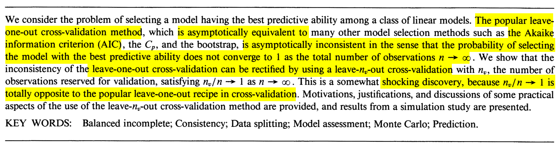
Figure 3.4: The abstract of Jun Shao’s Linear model selection by cross-validation (Shao 1993).

The Leave-One-Out Cross-Validation (LOOCV) error in a fitted linear model is defined as \[\begin{align} \mathrm{LOOCV}:=\frac{1}{n}\sum_{i=1}^n(Y_i-\hat{Y}_{i,-i})^2,\tag{3.3} \end{align}\] where \(\hat{Y}_{i,-i}\) is the prediction of the \(i\)-th observation in a linear model that has been fitted without the \(i\)-th datum \((X_{i1},\ldots,X_{ip},Y_i).\) That is, \(\hat{Y}_{i,-i}=\hat{\beta}_{0,-i}+\hat{\beta}_{1,-i}X_{i1}+\cdots+\hat{\beta}_{p,-i}X_{ip},\) where \(\hat{\boldsymbol{\beta}}_{-i}\) are the estimated coefficients from the sample \(\{(X_{j1},\ldots,X_{jp},Y_j)\}_{j=1,\, j\neq i}^n.\) Model selection based on LOOCV chooses the model with minimum error (3.3) within a list of candidate models. Note that the computation of \(\mathrm{LOOCV}\) requires, in principle, to fit \(n\) separate linear models, predict, and then aggregate. However, an algebraic shortcut based on (4.25) allows us to compute (3.3) using a single linear fit.

We carry out a small simulation study in order to illustrate the consistency property (3.2) of BIC and the inconsistency of model selection by AIC and LOOCV. For that, we consider the linear model \[\begin{align} \begin{split} Y&=\beta_0+\beta_1X_1+\beta_2X_2+\beta_3X_3+\beta_4X_4+\beta_5X_5+\varepsilon,\\ \boldsymbol{\beta}&=(0.5,1,1,0,0,0)^\top, \end{split} \tag{3.4} \end{align}\] where \(X_j\sim\mathcal{N}(0,1)\) for \(j=1,\ldots,5\) (independently) and \(\varepsilon\sim\mathcal{N}(0,1).\) Only the first two predictors are relevant, the last three are “garbage” predictors. For a given sample, model selection is performed by selecting among the \(2^5\) possible fitted models the ones with minimum AIC, BIC, and LOOCV. The experiment is repeated \(M=500\) times for sample sizes \(n=2^\ell,\) \(\ell=3,\ldots,12,\) and the estimated probability of selecting the correct model (the one only involving \(X_1\) and \(X_2\)) is displayed in Figure 3.5. The figure evidences empirically several interesting results:

• LOOCV and AIC are asymptotically equivalent. For large \(n,\) they tend to select the same model and hence their estimated probabilities of selecting the true model are almost equal. For small \(n,\) there are significant differences between them.
• The BIC is consistent in selecting the true model, and its probability of doing so quickly approaches \(1,\) as anticipated by (3.2).
• The AIC and LOOCV are inconsistent in selecting the true model. Despite the sample size \(n\) doubling at each step, their probability of recovering the true model gets stuck at about \(0.60.\)
• Even for moderate \(n\)’s, the probability of recovering the true model by BIC quickly outperforms those of AIC/LOOCV.

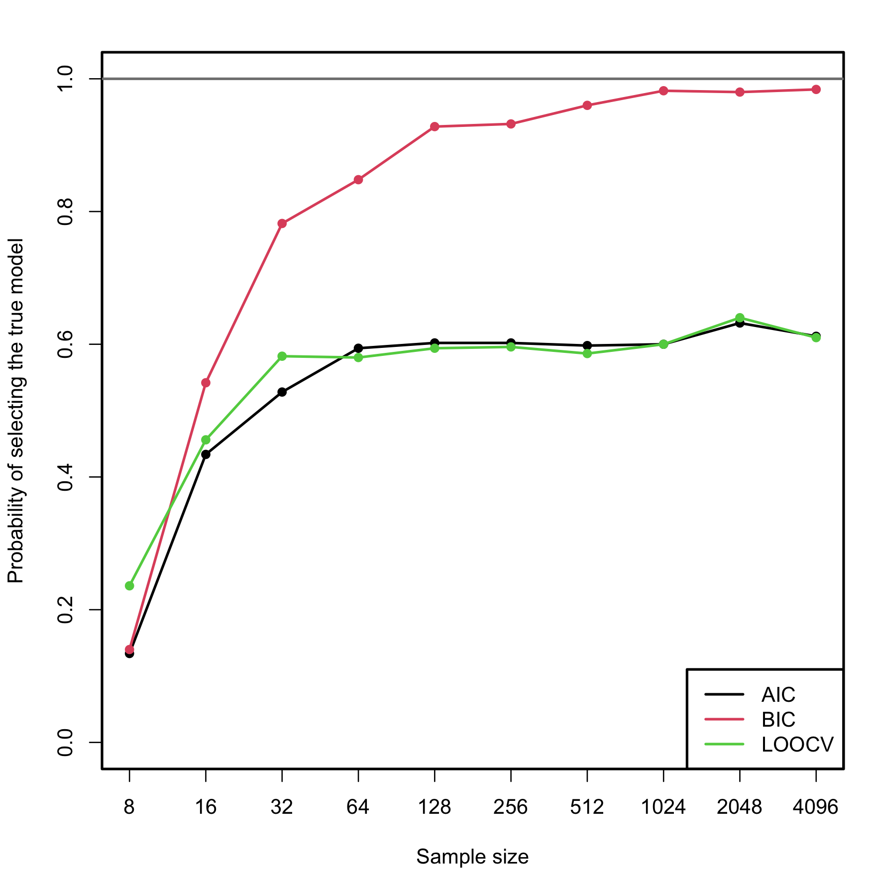
Figure 3.5: Estimation of the probability of selecting the correct model by minimizing the AIC, BIC, and LOOCV criteria, done for an exhaustive search with \(p=5\) predictors. The correct model contained two predictors. The probability was estimated with \(M=500\) Monte Carlo runs. The horizontal axis is in logarithmic scale. The estimated proportion of true model recoveries with BIC for \(n=4096\) is \(0.984\).

Exercise 3.3 Implement the simulation study behind Figure 3.5:

1. Sample from (3.4), but take \(p=4.\)
2. Fit the \(2^p\) possible models.
3. Select the best model according to the AIC and BIC.
4. Repeat Steps 1–3 \(M=100\) times. Estimate by Monte Carlo the probability of selecting the true model.
5. Move \(n\) in a range from \(10\) to \(200.\)

Once you have a working solution, increase \((p, n, M)\) to approach the settings in Figure 3.5 (or go beyond!).

Exercise 3.4 Modify the Step 3 of the previous exercise to:

1. Select the best model according to the \(R^2_\text{Adj}\) and investigate its consistency in model selection.
2. Add the LOOCV criterion in order to fully replicate Figure 3.5. Hint: you may want to adapt (4.25) to your needs in order to reduce computation time.

Exercise 3.5 Investigate what happens with the probability of selecting the true model using BIC and AIC if the exhaustive search is replaced by a stepwise selection. Precisely, do:

1. Sample from (3.4), but take \(p=10\) (pad \(\boldsymbol{\beta}\) with zeros).
2. Run a forward-backward stepwise search, both for the AIC and BIC.
3. Repeat Steps 1–2 \(M=100\) times. Estimate by Monte Carlo the probability of selecting the true model.
4. Move \(n\) in a range from \(20\) to \(200.\)

Once you have a working solution, increase \((n, M)\) to approach the settings in Figure 3.5 (or go beyond!).

Shao (1993)’s modification on how to make consistent the model selection by cross-validation is shocking. As in LOOCV, one has to split the sample of size \(n\) into two subsets: a training set, of size \(n_t,\) and a validation set, of size \(n_v.\) Of course, \(n=n_t+n_v.\) However, totally opposite to LOOCV, where \(n_t=n-1\) and \(n_v=1,\) the modification required is to choose \(n_v\) asymptotically equal to \(n\), in the sense that \(n_v/n\to1\) as \(n\to\infty.\) An example would be to take \(n_v=n-20\) and \(n_t=20.\) But \(n_v=n/2\) and \(n_t=n/2,\) a typical choice, would not make the selection consistent! Shao (1993)’s result gives a great insight: the difficulty in model selection lies in the comparison of models, not in their estimation, and the sample information has to be disproportionately allocated to the comparison task to achieve a consistent model selection device.

Exercise 3.6 Verify Shao (1993)’s result by constructing the analogous of Figure 3.5 for the following choices of \((n_t,n_v)\):

1. \(n_t=n-1,\) \(n_v=1\) (LOOCV).
2. \(n_t=n/2,\) \(n_v=n/2.\)
3. \(n_t=n/4,\) \(n_v=(3/4)n.\)
4. \(n_t=5p,\) \(n_v=n-5p.\)

Use first \(p=4\) predictors, \(M=100\) Monte Carlo runs, and move \(n\) in a range from \(20\) to \(200.\) Then increase the settings to approach those of Figure 3.5.

3.3 Use of qualitative predictors

An important situation not covered so far is how to deal with qualitative, and not quantitative, predictors. Qualitative predictors are also known as categorical variables or, in R’s terminology, factors, and are very common in many fields, such as in social sciences. Dealing with them requires some care and proper understanding of how these variables are represented.

The simplest case is the situation with two levels. A binary variable \(C\) with two levels (for example, a and b) can be encoded as

\[\begin{align*} D=\left\{\begin{array}{ll} 1,&\text{if }C=b,\\ 0,&\text{if }C=a. \end{array}\right. \end{align*}\]

\(D\) is a dummy variable: it codifies with zeros and ones the two possible levels of the categorical variable. An example of \(C\) is smoker, which has levels yes and no. The dummy variable associated is \(D=1\) if a person smokes and \(D=0\) if a person is non-smoker.

The advantage of this dummification is its interpretability in regression models. Since level a corresponds to \(0,\) it can be seen as the reference level to which level b is compared. This is the key point in dummification: set one level as the reference, codify the rest as departures from it.

The previous interpretation translates easily to the linear model. Assume that the dummy variable \(D\) is available together with other predictors \(X_1,\ldots,X_p.\) Then:

\[\begin{align*} \mathbb{E}[Y \mid X_1=x_1,\ldots,X_p=x_p,D=d]=\beta_0+\beta_1x_1+\cdots+\beta_px_p+\beta_{p+1}d. \end{align*}\]

The coefficient associated with \(D\) is easily interpretable: \(\beta_{p+1}\) is the increment in the mean of \(Y\) associated with changing \(D=0\) (reference) to \(D=1,\) while the rest of the predictors are fixed. Or in other words, \(\beta_{p+1}\) is the increment in the mean of \(Y\) associated with changing the level of the categorical variable from a to b.

R does the dummification automatically, translating a categorical variable \(C\) into its dummy version \(D,\) if it detects that a factor variable is present in the regression model.

Let’s see now the case with more than two levels, for example, a categorical variable \(C\) with levels a, b, and c. If we take a as the reference level, this variable can be represented by two dummy variables:

\[\begin{align*} D_1=\left\{\begin{array}{ll}1,&\text{if }C=b,\\0,& \text{if }C\neq b\end{array}\right. \end{align*}\]

and

\[\begin{align*} D_2=\left\{\begin{array}{ll}1,&\text{if }C=c,\\0,& \text{if }C\neq c.\end{array}\right. \end{align*}\]

Therefore, we can represent the levels of \(C\) as in the following table.

\(C\)	\(D_1\)	\(D_2\)
\(a\)	\(0\)	\(0\)
\(b\)	\(1\)	\(0\)
\(c\)	\(0\)	\(1\)

The interpretation of the regression models in the presence of \(D_1\) and \(D_2\) is very similar to the one before. For example, for the linear model, the coefficient associated with \(D_1\) gives the increment in the mean of \(Y\) when the level of \(C\) changes from a to b, and the coefficient for \(D_2\) gives the increment in the mean of \(Y\) when \(C\) changes from a to c.

In general, if we have a categorical variable \(C\) with \(J\) levels, then the previous process is iterated and the number of dummy variables required to encode \(C\) is \(J-1\;\)⁶³. Again, R does the dummification automatically if it detects that a factor variable is present in the regression model.

Let’s see an example with the famous iris dataset.

# iris dataset -- factors in the last column
summary(iris)
##   Sepal.Length    Sepal.Width     Petal.Length    Petal.Width          Species  
##  Min.   :4.300   Min.   :2.000   Min.   :1.000   Min.   :0.100   setosa    :50  
##  1st Qu.:5.100   1st Qu.:2.800   1st Qu.:1.600   1st Qu.:0.300   versicolor:50  
##  Median :5.800   Median :3.000   Median :4.350   Median :1.300   virginica :50  
##  Mean   :5.843   Mean   :3.057   Mean   :3.758   Mean   :1.199                  
##  3rd Qu.:6.400   3rd Qu.:3.300   3rd Qu.:5.100   3rd Qu.:1.800                  
##  Max.   :7.900   Max.   :4.400   Max.   :6.900   Max.   :2.500

# Summary of a linear model
mod1 <- lm(Sepal.Length ~ ., data = iris)
summary(mod1)
## 
## Call:
## lm(formula = Sepal.Length ~ ., data = iris)
## 
## Residuals:
##      Min       1Q   Median       3Q      Max 
## -0.79424 -0.21874  0.00899  0.20255  0.73103 
## 
## Coefficients:
##                   Estimate Std. Error t value Pr(>|t|)    
## (Intercept)        2.17127    0.27979   7.760 1.43e-12 ***
## Sepal.Width        0.49589    0.08607   5.761 4.87e-08 ***
## Petal.Length       0.82924    0.06853  12.101  < 2e-16 ***
## Petal.Width       -0.31516    0.15120  -2.084  0.03889 *  
## Speciesversicolor -0.72356    0.24017  -3.013  0.00306 ** 
## Speciesvirginica  -1.02350    0.33373  -3.067  0.00258 ** 
## ---
## Signif. codes:  0 '***' 0.001 '**' 0.01 '*' 0.05 '.' 0.1 ' ' 1
## 
## Residual standard error: 0.3068 on 144 degrees of freedom
## Multiple R-squared:  0.8673, Adjusted R-squared:  0.8627 
## F-statistic: 188.3 on 5 and 144 DF,  p-value: < 2.2e-16
# Speciesversicolor (D1) coefficient: -0.72356. The average increment of
# Sepal.Length when the species is versicolor instead of setosa (reference)
# Speciesvirginica (D2) coefficient: -1.02350. The average increment of
# Sepal.Length when the species is virginica instead of setosa (reference)
# Both dummy variables are significant

# How to set a different level as reference (versicolor)
iris$Species <- relevel(iris$Species, ref = "versicolor")

# Same estimates, except for the dummy coefficients
mod2 <- lm(Sepal.Length ~ ., data = iris)
summary(mod2)
## 
## Call:
## lm(formula = Sepal.Length ~ ., data = iris)
## 
## Residuals:
##      Min       1Q   Median       3Q      Max 
## -0.79424 -0.21874  0.00899  0.20255  0.73103 
## 
## Coefficients:
##                  Estimate Std. Error t value Pr(>|t|)    
## (Intercept)       1.44770    0.28149   5.143 8.68e-07 ***
## Sepal.Width       0.49589    0.08607   5.761 4.87e-08 ***
## Petal.Length      0.82924    0.06853  12.101  < 2e-16 ***
## Petal.Width      -0.31516    0.15120  -2.084  0.03889 *  
## Speciessetosa     0.72356    0.24017   3.013  0.00306 ** 
## Speciesvirginica -0.29994    0.11898  -2.521  0.01280 *  
## ---
## Signif. codes:  0 '***' 0.001 '**' 0.01 '*' 0.05 '.' 0.1 ' ' 1
## 
## Residual standard error: 0.3068 on 144 degrees of freedom
## Multiple R-squared:  0.8673, Adjusted R-squared:  0.8627 
## F-statistic: 188.3 on 5 and 144 DF,  p-value: < 2.2e-16
# Speciessetosa (D1) coefficient: 0.72356. The average increment of
# Sepal.Length when the species is setosa instead of versicolor (reference)
# Speciesvirginica (D2) coefficient: -0.29994. The average increment of
# Sepal.Length when the species is virginica instead of versicolor (reference)
# Both dummy variables are significant

# Coefficients of the model
confint(mod2)
##                       2.5 %      97.5 %
## (Intercept)       0.8913266  2.00408209
## Sepal.Width       0.3257653  0.66601260
## Petal.Length      0.6937939  0.96469395
## Petal.Width      -0.6140049 -0.01630542
## Speciessetosa     0.2488500  1.19827390
## Speciesvirginica -0.5351144 -0.06475727
# The coefficients of Speciessetosa and Speciesvirginica are
# significantly positive and negative, respectively

# Show the dummy variables employed for encoding a factor
contrasts(iris$Species)
##            setosa virginica
## versicolor      0         0
## setosa          1         0
## virginica       0         1
iris$Species <- relevel(iris$Species, ref = "setosa")
contrasts(iris$Species)
##            versicolor virginica
## setosa              0         0
## versicolor          1         0
## virginica           0         1

It may happen that one dummy variable, say \(D_1,\) is not significant, while other dummy variables of the same categorical variable, say \(D_2,\) are significant. For example, this happens in the example above at level \(\alpha=0.01.\) Then, in the considered model, the level associated with \(D_1\) does not add relevant information for explaining \(Y\) with respect to the reference level.

Do not codify a categorical variable as a discrete variable. This constitutes a major methodological failure that will flaw the subsequent statistical analysis.

For example if you have a categorical variable party with levels partyA, partyB, and partyC, do not encode it as a discrete variable taking the values 1, 2, and 3, respectively. If you do so:

• You assume implicitly an order in the levels of party, since partyA is closer to partyB than to partyC.
• You assume implicitly that partyC is three times larger than partyA.
• The codification is completely arbitrary – why not consider 1, 1.5, and 1.75 instead?

The right way of dealing with categorical variables in regression is to set the variable as a factor and let R do the dummification internally.

3.3.1 Case study application

Let’s see what the dummy variables are in the Boston dataset and what effect they have on medv.

# Load the Boston dataset
data(Boston, package = "MASS")

# Structure of the data
str(Boston)
## 'data.frame':    506 obs. of  14 variables:
##  $ crim   : num  0.00632 0.02731 0.02729 0.03237 0.06905 ...
##  $ zn     : num  18 0 0 0 0 0 12.5 12.5 12.5 12.5 ...
##  $ indus  : num  2.31 7.07 7.07 2.18 2.18 2.18 7.87 7.87 7.87 7.87 ...
##  $ chas   : int  0 0 0 0 0 0 0 0 0 0 ...
##  $ nox    : num  0.538 0.469 0.469 0.458 0.458 0.458 0.524 0.524 0.524 0.524 ...
##  $ rm     : num  6.58 6.42 7.18 7 7.15 ...
##  $ age    : num  65.2 78.9 61.1 45.8 54.2 58.7 66.6 96.1 100 85.9 ...
##  $ dis    : num  4.09 4.97 4.97 6.06 6.06 ...
##  $ rad    : int  1 2 2 3 3 3 5 5 5 5 ...
##  $ tax    : num  296 242 242 222 222 222 311 311 311 311 ...
##  $ ptratio: num  15.3 17.8 17.8 18.7 18.7 18.7 15.2 15.2 15.2 15.2 ...
##  $ black  : num  397 397 393 395 397 ...
##  $ lstat  : num  4.98 9.14 4.03 2.94 5.33 ...
##  $ medv   : num  24 21.6 34.7 33.4 36.2 28.7 22.9 27.1 16.5 18.9 ...
# chas is a dummy variable measuring if the suburb is close to the river (1)
# or not (0). In this case it is not codified as a factor but as a 0 or 1
# (so it is already dummified)

# Summary of a linear model
mod <- lm(medv ~ chas + crim, data = Boston)
summary(mod)
## 
## Call:
## lm(formula = medv ~ chas + crim, data = Boston)
## 
## Residuals:
##     Min      1Q  Median      3Q     Max 
## -16.540  -5.421  -1.878   2.575  30.134 
## 
## Coefficients:
##             Estimate Std. Error t value Pr(>|t|)    
## (Intercept) 23.61403    0.41862  56.409  < 2e-16 ***
## chas         5.57772    1.46926   3.796 0.000165 ***
## crim        -0.40598    0.04339  -9.358  < 2e-16 ***
## ---
## Signif. codes:  0 '***' 0.001 '**' 0.01 '*' 0.05 '.' 0.1 ' ' 1
## 
## Residual standard error: 8.373 on 503 degrees of freedom
## Multiple R-squared:  0.1744, Adjusted R-squared:  0.1712 
## F-statistic: 53.14 on 2 and 503 DF,  p-value: < 2.2e-16
# The coefficient associated with `chas` is 5.57772. That means that if the suburb
# is close to the river, the mean of medv increases in 5.57772 units for
# the same house and neighborhood conditions
# chas is significant (the presence of the river adds a valuable information
# for explaining medv)

# Summary of the best model in terms of BIC
summary(modBIC)
## 
## Call:
## lm(formula = medv ~ crim + zn + chas + nox + rm + dis + rad + 
##     tax + ptratio + black + lstat, data = Boston)
## 
## Residuals:
##      Min       1Q   Median       3Q      Max 
## -15.5984  -2.7386  -0.5046   1.7273  26.2373 
## 
## Coefficients:
##               Estimate Std. Error t value Pr(>|t|)    
## (Intercept)  36.341145   5.067492   7.171 2.73e-12 ***
## crim         -0.108413   0.032779  -3.307 0.001010 ** 
## zn            0.045845   0.013523   3.390 0.000754 ***
## chas          2.718716   0.854240   3.183 0.001551 ** 
## nox         -17.376023   3.535243  -4.915 1.21e-06 ***
## rm            3.801579   0.406316   9.356  < 2e-16 ***
## dis          -1.492711   0.185731  -8.037 6.84e-15 ***
## rad           0.299608   0.063402   4.726 3.00e-06 ***
## tax          -0.011778   0.003372  -3.493 0.000521 ***
## ptratio      -0.946525   0.129066  -7.334 9.24e-13 ***
## black         0.009291   0.002674   3.475 0.000557 ***
## lstat        -0.522553   0.047424 -11.019  < 2e-16 ***
## ---
## Signif. codes:  0 '***' 0.001 '**' 0.01 '*' 0.05 '.' 0.1 ' ' 1
## 
## Residual standard error: 4.736 on 494 degrees of freedom
## Multiple R-squared:  0.7406, Adjusted R-squared:  0.7348 
## F-statistic: 128.2 on 11 and 494 DF,  p-value: < 2.2e-16
# The coefficient associated with `chas` is 2.71871. If the suburb is close to
# the river, the mean of medv increases in 2.71871 units
# chas is significant as well in the presence of more predictors

We will see how to mix dummy and quantitative predictors in Section 3.4.3.

3.4 Nonlinear relationships

3.4.1 Transformations in the simple linear model

The linear model is termed linear not only because the form it assumes for the regression function \(m\) is linear, but because the effects of the parameters are linear. Indeed, the predictor \(X\) may exhibit a nonlinear effect on the response \(Y\) and still be a linear model! For example, the following models can be transformed into simple linear models:

1. \(Y=\beta_0+\beta_1X^2+\varepsilon.\)
2. \(Y=\beta_0+\beta_1\log(X)+\varepsilon.\)
3. \(Y=\beta_0+\beta_1(X^3-\log(|X|) + 2^{X})+\varepsilon.\)

The trick is to work with a transformed predictor \(\tilde{X}\) as a replacement of the original predictor \(X.\) Then, for the above examples, rather than working with the sample \(\{(X_i,Y_i)\}_{i=1}^n,\) we consider the transformed sample \(\{(\tilde X_i,Y_i)\}_{i=1}^n\) with:

1. \(\tilde X_i=X_i^2,\) \(i=1,\ldots,n.\)
2. \(\tilde X_i=\log(X_i),\) \(i=1,\ldots,n.\)
3. \(\tilde X_i=X_i^3-\log(|X_i|) + 2^{X_i},\) \(i=1,\ldots,n.\)

An example of this simple but powerful trick is given as follows. The left panel of Figure 3.6 shows the scatterplot for some data y and x, together with its fitted regression line. Clearly, the data does not follow a linear pattern, but a nonlinear one, similar to a parabola \(y=x^2.\) Hence, y might be better explained by the square of x, x^2, rather than by x. Indeed, if we plot y against x^2 in the right panel of Figure 3.6, we can see that the relation of y and x^2 is now linear!

Figure 3.6: Left: quadratic pattern when plotting \(Y\) against \(X.\) Right: linearized pattern when plotting \(Y\) against \(X^2.\) In red, the fitted regression line.

Figure 3.7: Illustration of the choice of the nonlinear transformation. Application available here.

In conclusion, with a simple trick we have drastically increased the explanation of the response. However, there is a catch: knowing which transformation is required in order to linearize the relation between response and the predictor is a kind of art which requires good eyeballing. A first approach is to try with one of the usual transformations, displayed in Figure 3.8, depending on the pattern of the data. Figure 3.7 illustrates how to choose an adequate transformation for linearizing certain nonlinear data patterns.

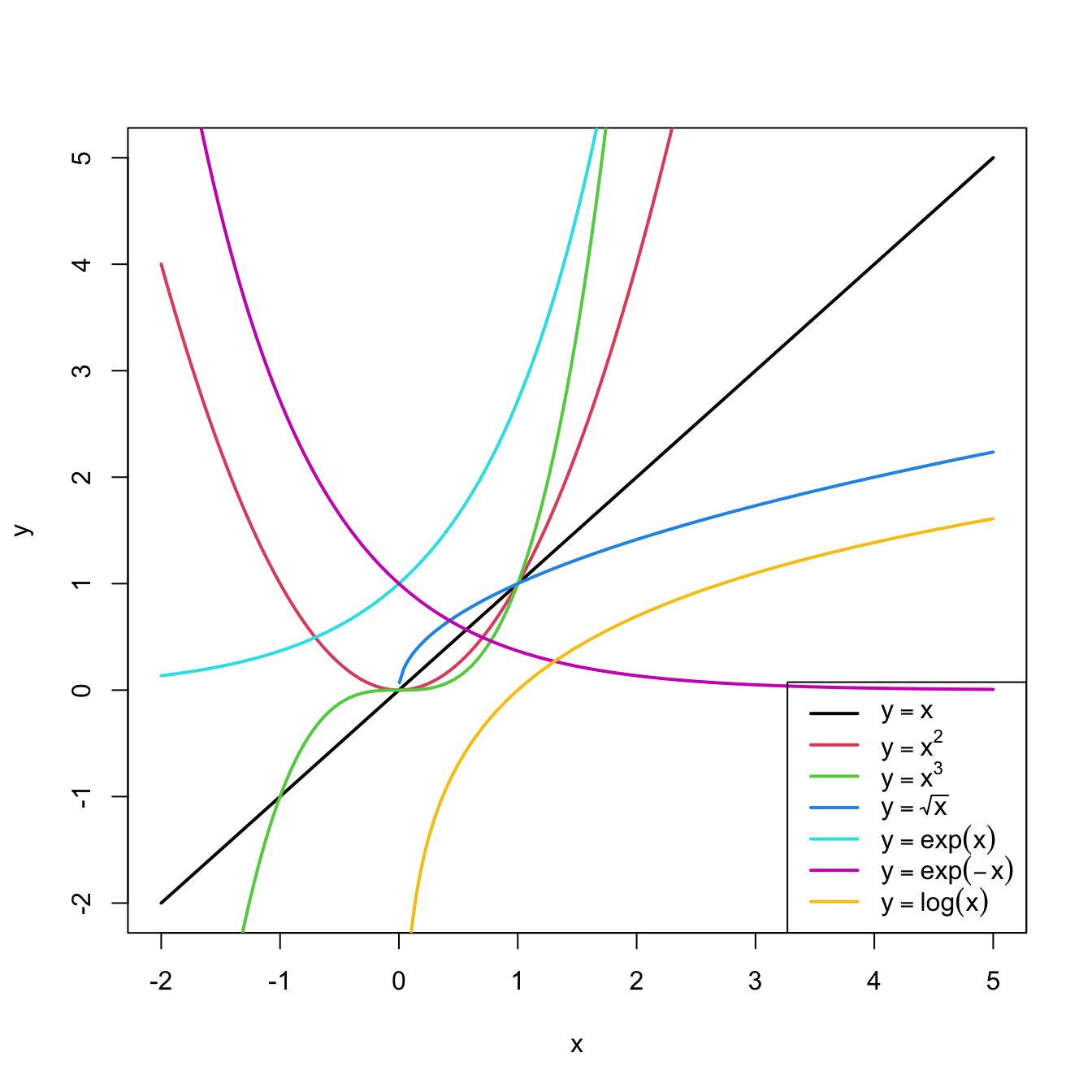
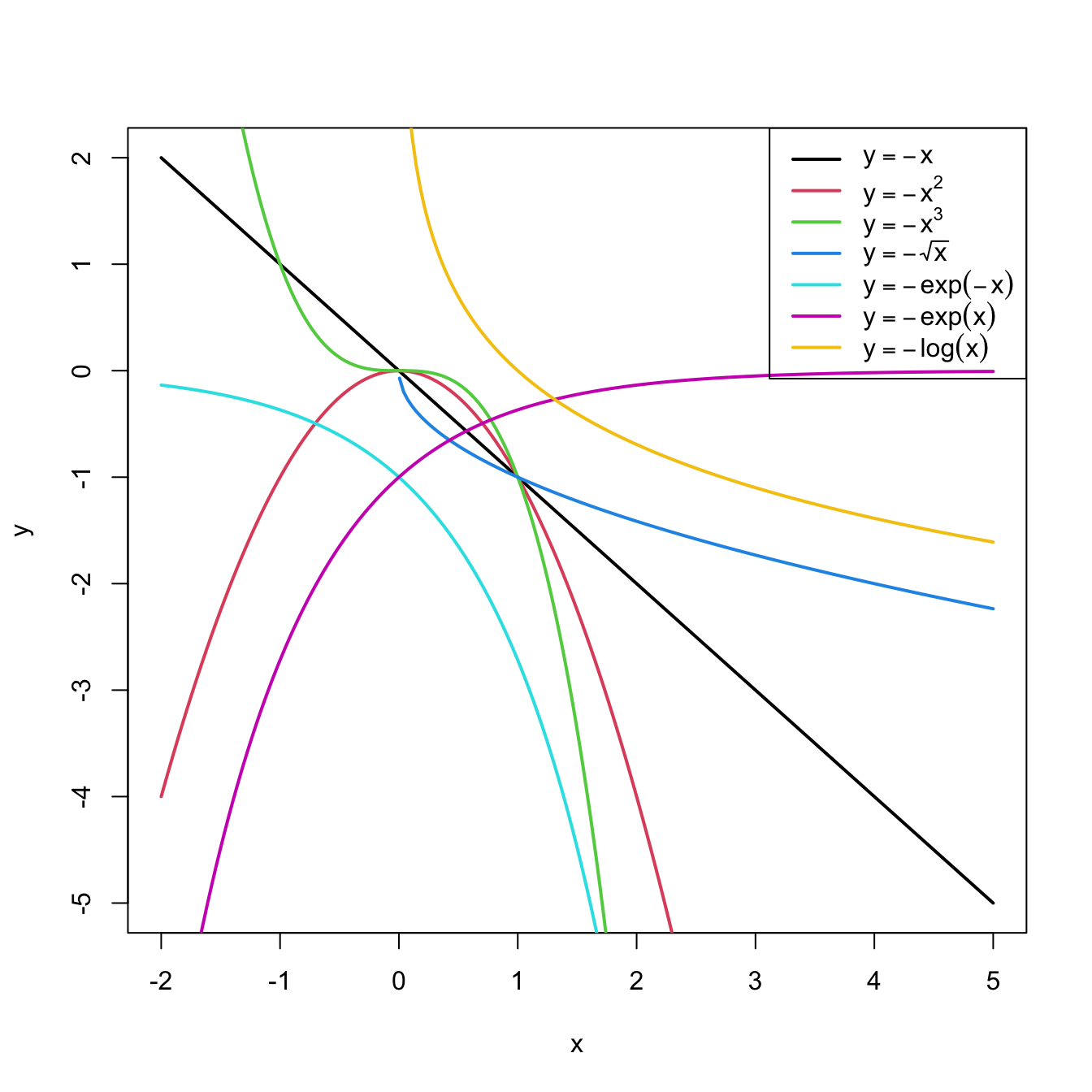
Figure 3.8: Some common nonlinear transformations and their negative counterparts. Recall the domain of definition of each transformation.

If you apply a nonlinear transformation, namely \(f,\) and fit the linear model \(Y=\beta_0+\beta_1 f(X)+\varepsilon,\) then there is no point in also fitting the model resulting from the negative transformation \(-f.\) The model with \(-f\) is exactly the same as the one with \(f\) but with the sign of \(\beta_1\) flipped.

As a rule of thumb, use Figure 3.8 with the transformations to compare it with the data pattern, choose the most similar curve, and apply the corresponding function with positive sign (for simpler interpretation).

Let’s see how to transform the predictor and perform the regressions behind Figure 3.6.

# Data
x <- c(-2, -1.9, -1.7, -1.6, -1.4, -1.3, -1.1, -1, -0.9, -0.7, -0.6,
       -0.4, -0.3, -0.1, 0, 0.1, 0.3, 0.4, 0.6, 0.7, 0.9, 1, 1.1, 1.3,
       1.4, 1.6, 1.7, 1.9, 2, 2.1, 2.3, 2.4, 2.6, 2.7, 2.9, 3, 3.1,
       3.3, 3.4, 3.6, 3.7, 3.9, 4, 4.1, 4.3, 4.4, 4.6, 4.7, 4.9, 5)
y <- c(1.4, 0.4, 2.4, 1.7, 2.4, 0, 0.3, -1, 1.3, 0.2, -0.7, 1.2, -0.1,
       -1.2, -0.1, 1, -1.1, -0.9, 0.1, 0.8, 0, 1.7, 0.3, 0.8, 1.2, 1.1,
       2.5, 1.5, 2, 3.8, 2.4, 2.9, 2.7, 4.2, 5.8, 4.7, 5.3, 4.9, 5.1,
       6.3, 8.6, 8.1, 7.1, 7.9, 8.4, 9.2, 12, 10.5, 8.7, 13.5)

# Data frame (a matrix with column names)
nonLinear <- data.frame(x = x, y = y)

# We create a new column inside nonLinear, called x2, that contains the
# new variable x^2
nonLinear$x2 <- nonLinear$x^2
# If you wish to remove it
# nonLinear$x2 <- NULL

# Regressions
mod1 <- lm(y ~ x, data = nonLinear)
mod2 <- lm(y ~ x2, data = nonLinear)
summary(mod1)
## 
## Call:
## lm(formula = y ~ x, data = nonLinear)
## 
## Residuals:
##     Min      1Q  Median      3Q     Max 
## -2.5268 -1.7513 -0.4017  0.9750  5.0265 
## 
## Coefficients:
##             Estimate Std. Error t value Pr(>|t|)    
## (Intercept)   0.9771     0.3506   2.787   0.0076 ** 
## x             1.4993     0.1374  10.911 1.35e-14 ***
## ---
## Signif. codes:  0 '***' 0.001 '**' 0.01 '*' 0.05 '.' 0.1 ' ' 1
## 
## Residual standard error: 2.005 on 48 degrees of freedom
## Multiple R-squared:  0.7126, Adjusted R-squared:  0.7067 
## F-statistic:   119 on 1 and 48 DF,  p-value: 1.353e-14
summary(mod2)
## 
## Call:
## lm(formula = y ~ x2, data = nonLinear)
## 
## Residuals:
##     Min      1Q  Median      3Q     Max 
## -3.0418 -0.5523 -0.1465  0.6286  1.8797 
## 
## Coefficients:
##             Estimate Std. Error t value Pr(>|t|)    
## (Intercept)  0.05891    0.18462   0.319    0.751    
## x2           0.48659    0.01891  25.725   <2e-16 ***
## ---
## Signif. codes:  0 '***' 0.001 '**' 0.01 '*' 0.05 '.' 0.1 ' ' 1
## 
## Residual standard error: 0.9728 on 48 degrees of freedom
## Multiple R-squared:  0.9324, Adjusted R-squared:  0.931 
## F-statistic: 661.8 on 1 and 48 DF,  p-value: < 2.2e-16
# mod2 has a larger R^2. Also notice the intercept is not significant

A fast way of performing and summarizing the quadratic fit is

summary(lm(y ~ I(x^2), data = nonLinear))

The I() function wrapping x^2 is fundamental when applying arithmetic operations in the predictor. The symbols +, *, ^, … have different meaning when inputted in a formula, so it is required to use I() to indicate that they must be interpreted in their arithmetic meaning and that the result of the expression denotes a new predictor. For example, use I((x - 1)^3 - log(3 * x)) to apply the transformation (x - 1)^3 - log(3 * x).

Exercise 3.7 Load the dataset assumptions.RData. We are going to work with the regressions y2 ~ x2, y3 ~ x3, y8 ~ x8, and y9 ~ x9, in order to identify which transformation of Figure 3.8 gives the best fit. For these, do the following:

1. Find the transformation that yields the largest \(R^2.\)
2. Compare the original and transformed linear models.

Hints:

• y2 ~ x2 has a negative dependence, so look at the right panel of Figure 3.7.
• y3 ~ x3 seems to have just a subtle nonlinearity… Will it be worth to attempt a transformation?
• For y9 ~ x9, try also with exp(-abs(x9)), log(abs(x9)), and 2^abs(x9).

The nonlinear transformations introduced for the simple linear model are readily applicable in the multiple linear model. Consequently, the multiple linear model is able to approximate regression functions with nonlinear forms, if appropriate nonlinear transformations for the predictors are used.⁶⁴

3.4.2 Polynomial transformations

Polynomial models are a powerful nonlinear extension of the linear model. These are constructed by replacing each predictor \(X_j\) by a set of monomials \((X_j,X_j^2,\ldots,X_j^{k_j})\) constructed from \(X_j.\) In the simpler case with a single predictor⁶⁵ \(X,\) we have the \(k\)-th order polynomial fit:

\[\begin{align*} Y=\beta_0+\beta_1X+\cdots+\beta_kX^k+\varepsilon. \end{align*}\]

With this approach, a highly flexible model is produced, as it was already shown in Figure 1.3.

The creation of polynomial models can be automated with the R’s poly function. For the observations \((X_1,\ldots,X_n)\) of \(X,\) poly creates the matrices

\[\begin{align} \begin{pmatrix} X_{1} & X_{1}^2 & \ldots & X_{1}^k \\ \vdots & \vdots & \ddots & \vdots \\ X_{n} & X_{n}^2 & \ldots & X_{n}^k \\ \end{pmatrix}\text{ or } \begin{pmatrix} p_1(X_{1}) & p_2(X_{1}) & \ldots & p_k(X_{1}) \\ \vdots & \vdots & \ddots & \vdots \\ p_1(X_{n}) & p_2(X_{n}) & \ldots & p_k(X_{n}) \\ \end{pmatrix},\tag{3.5} \end{align}\]

where \(p_1,\ldots,p_k\) are orthogonal polynomials⁶⁶ of orders \(1,\ldots,k,\) respectively. For orthogonal polynomials, poly yields a data matrix in (3.5) with uncorrelated⁶⁷ columns. That is, such that the sample correlation coefficient between two columns is zero.

Let’s see a couple of examples on using poly.

x1 <- seq(-1, 1, l = 4)
poly(x = x1, degree = 2, raw = TRUE) # (X, X^2)
##               1         2
## [1,] -1.0000000 1.0000000
## [2,] -0.3333333 0.1111111
## [3,]  0.3333333 0.1111111
## [4,]  1.0000000 1.0000000
## attr(,"degree")
## [1] 1 2
## attr(,"class")
## [1] "poly"   "matrix"
poly(x = x1, degree = 2) # By default, it employs orthogonal polynomials
##               1    2
## [1,] -0.6708204  0.5
## [2,] -0.2236068 -0.5
## [3,]  0.2236068 -0.5
## [4,]  0.6708204  0.5
## attr(,"coefs")
## attr(,"coefs")$alpha
## [1] -5.551115e-17 -5.551115e-17
## 
## attr(,"coefs")$norm2
## [1] 1.0000000 4.0000000 2.2222222 0.7901235
## 
## attr(,"degree")
## [1] 1 2
## attr(,"class")
## [1] "poly"   "matrix"

# Depiction of raw polynomials
x <- seq(-1, 1, l = 200)
degree <- 5
matplot(x, poly(x, degree = degree, raw = TRUE), type = "l", lty = 1,
        ylab = expression(x^k))
legend("bottomright", legend = paste("k =", 1:degree), col = 1:degree, lwd = 2)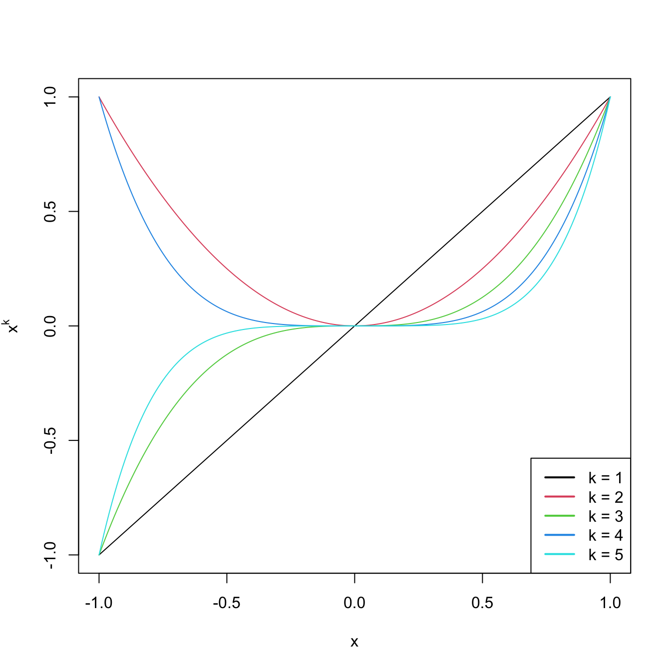

Figure 3.9: Raw polynomials \(x^k\) in \((-1,1),\) up to degree \(k=5.\)

# Depiction of orthogonal polynomials
matplot(x, poly(x, degree = degree), type = "l", lty = 1,
        ylab = expression(p[k](x)))
legend("bottomright", legend = paste("k =", 1:degree), col = 1:degree, lwd = 2)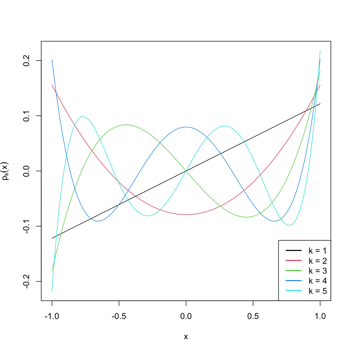

Figure 3.10: Orthogonal polynomials \(p_k(x)\) in \((-1,1),\) up to degree \(k=5.\)

These matrices can now be used as inputs in the predictor side of lm. Let’s see this in an example.

# Data containing speed (mph) and stopping distance (ft) of cars from 1920
data(cars)
plot(cars, xlab = "Speed (mph)", ylab = "Stopping distance (ft)")

# Fit a linear model of dist ~ speed
mod1 <- lm(dist ~ speed, data = cars)
abline(coef = mod1$coefficients, col = 2)

# Quadratic
mod2 <- lm(dist ~ poly(speed, degree = 2), data = cars)
# The fit is not a line, we must look for an alternative approach
d <- seq(0, 25, length.out = 200)
lines(d, predict(mod2, new = data.frame(speed = d)), col = 3)

# Cubic
mod3 <- lm(dist ~ poly(speed, degree = 3), data = cars)
lines(d, predict(mod3, new = data.frame(speed = d)), col = 4)

# 10th order -- overfitting
mod10 <- lm(dist ~ poly(speed, degree = 10), data = cars)
lines(d, predict(mod10, new = data.frame(speed = d)), col = 5)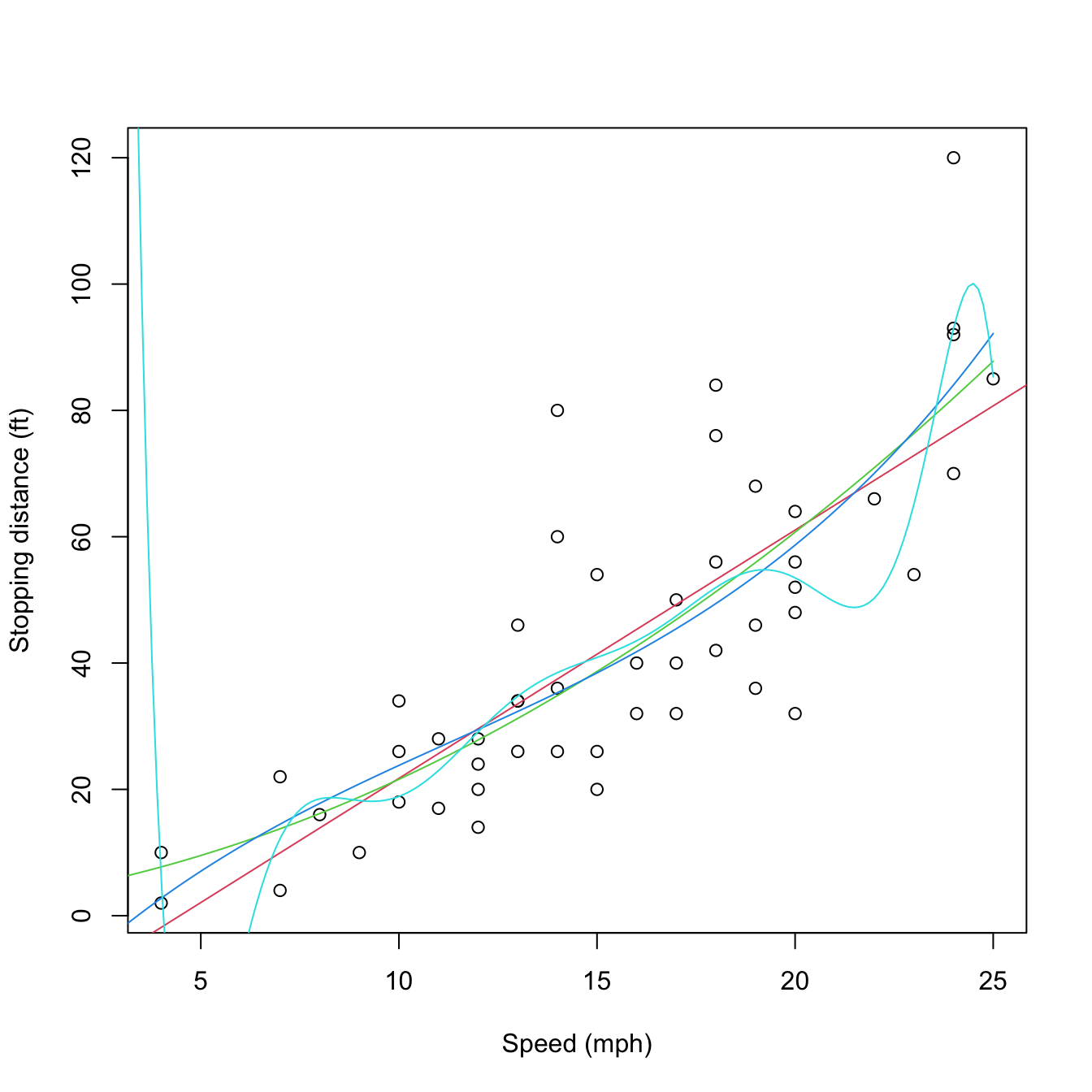

Figure 3.11: Raw and orthogonal polynomial fits of dist ~ speed in the cars dataset.

# BICs -- the linear model is better!
BIC(mod1, mod2, mod3, mod10)
##       df      BIC
## mod1   3 424.8929
## mod2   4 426.4202
## mod3   5 429.4451
## mod10 12 450.3523

# poly computes by default orthogonal polynomials. These are not
# X^1, X^2, ..., X^p but combinations of them such that the polynomials are
# orthogonal. 'Raw' polynomials are possible with raw = TRUE. They give the
# same fit, but the coefficient estimates are different.
mod2Raw <- lm(dist ~ poly(speed, degree = 2, raw = TRUE), data = cars)
plot(cars, xlab = "Speed (mph)", ylab = "Stopping distance (ft)")
lines(d, predict(mod2, new = data.frame(speed = d)), col = 1)
lines(d, predict(mod2Raw, new = data.frame(speed = d)), col = 2)

Figure 3.12: Raw and orthogonal polynomial fits of dist ~ speed in the cars dataset.

# However: different coefficient estimates, but same R^2. How is this possible?
summary(mod2)
## 
## Call:
## lm(formula = dist ~ poly(speed, degree = 2), data = cars)
## 
## Residuals:
##     Min      1Q  Median      3Q     Max 
## -28.720  -9.184  -3.188   4.628  45.152 
## 
## Coefficients:
##                          Estimate Std. Error t value Pr(>|t|)    
## (Intercept)                42.980      2.146  20.026  < 2e-16 ***
## poly(speed, degree = 2)1  145.552     15.176   9.591 1.21e-12 ***
## poly(speed, degree = 2)2   22.996     15.176   1.515    0.136    
## ---
## Signif. codes:  0 '***' 0.001 '**' 0.01 '*' 0.05 '.' 0.1 ' ' 1
## 
## Residual standard error: 15.18 on 47 degrees of freedom
## Multiple R-squared:  0.6673, Adjusted R-squared:  0.6532 
## F-statistic: 47.14 on 2 and 47 DF,  p-value: 5.852e-12
summary(mod2Raw)
## 
## Call:
## lm(formula = dist ~ poly(speed, degree = 2, raw = TRUE), data = cars)
## 
## Residuals:
##     Min      1Q  Median      3Q     Max 
## -28.720  -9.184  -3.188   4.628  45.152 
## 
## Coefficients:
##                                      Estimate Std. Error t value Pr(>|t|)
## (Intercept)                           2.47014   14.81716   0.167    0.868
## poly(speed, degree = 2, raw = TRUE)1  0.91329    2.03422   0.449    0.656
## poly(speed, degree = 2, raw = TRUE)2  0.09996    0.06597   1.515    0.136
## 
## Residual standard error: 15.18 on 47 degrees of freedom
## Multiple R-squared:  0.6673, Adjusted R-squared:  0.6532 
## F-statistic: 47.14 on 2 and 47 DF,  p-value: 5.852e-12

# Because the predictors in mod2Raw are highly related between them, and
# the ones in mod2 are uncorrelated between them!
car::scatterplotMatrix(mod2$model[, -1], col = 1, regLine = list(col = 2),
                       smooth = list(col.smooth = 4, col.spread = 4))
car::scatterplotMatrix(mod2Raw$model[, -1],col = 1, regLine = list(col = 2),
                       smooth = list(col.smooth = 4, col.spread = 4))
cor(mod2$model[, -1])
##   1 2
## 1 1 0
## 2 0 1
cor(mod2Raw$model[, -1])
##           1         2
## 1 1.0000000 0.9794765
## 2 0.9794765 1.0000000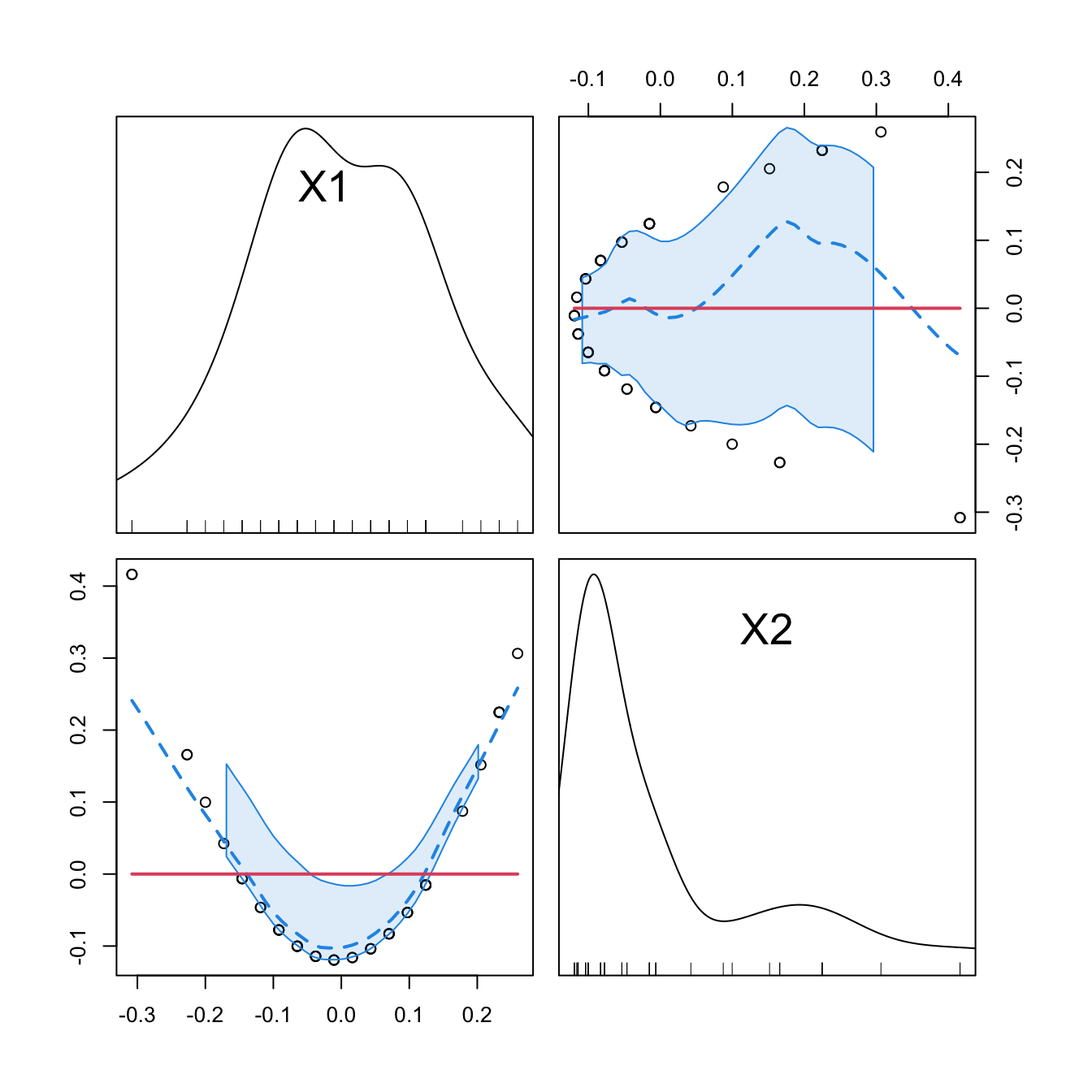

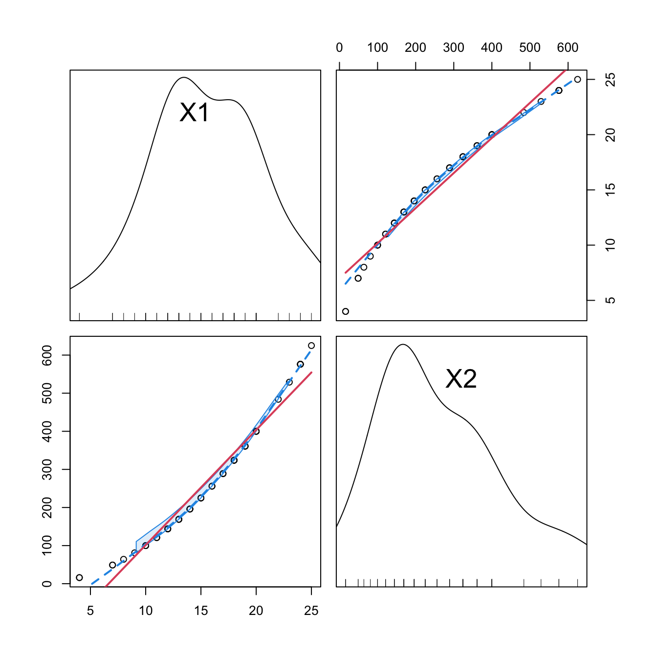
Figure 3.13: Correlations between the first and second order orthogonal polynomials associated to speed, and between speed and speed^2.

The use of orthogonal polynomials instead of raw polynomials is advised for high order polynomial fits, since they avoid the numerical instabilities arising from excessive linear dependencies between the raw polynomial predictors.

3.4.3 Interactions

When two or more predictors \(X_1\) and \(X_2\) are present, it may be of interest to explore the interaction between them by means of \(X_1X_2.\) This is a new variable that positively (negatively) affects the response \(Y\) when both \(X_1\) and \(X_2\) are positive or negative at the same time (at different times):

\[\begin{align*} Y=\beta_0+\beta_1X_1+\beta_2X_2+\beta_3X_1X_2+\varepsilon. \end{align*}\]

The coefficient \(\beta_3\) in \(Y=\beta_0+\beta_1X_1+\beta_2X_2+\beta_3X_1X_2+\varepsilon\) can be interpreted as the increment of the effect of the predictor \(X_1\) on the mean of \(Y,\) for a unit increment in \(X_2\).⁶⁸ Significance testing on these coefficients can be carried out as usual.

The way of adding these interactions in lm is through the operators : and *. The operator : only adds the term \(X_1X_2,\) while * adds \(X_1,\) \(X_2,\) and \(X_1X_2\) at the same time. Let’s see an example in the Boston dataset.

# Interaction between lstat and age
summary(lm(medv ~ lstat + lstat:age, data = Boston))
## 
## Call:
## lm(formula = medv ~ lstat + lstat:age, data = Boston)
## 
## Residuals:
##     Min      1Q  Median      3Q     Max 
## -15.815  -4.039  -1.335   2.086  27.491 
## 
## Coefficients:
##              Estimate Std. Error t value Pr(>|t|)    
## (Intercept) 36.041514   0.691334  52.133  < 2e-16 ***
## lstat       -1.388161   0.126911 -10.938  < 2e-16 ***
## lstat:age    0.004103   0.001133   3.621 0.000324 ***
## ---
## Signif. codes:  0 '***' 0.001 '**' 0.01 '*' 0.05 '.' 0.1 ' ' 1
## 
## Residual standard error: 6.142 on 503 degrees of freedom
## Multiple R-squared:  0.5557, Adjusted R-squared:  0.554 
## F-statistic: 314.6 on 2 and 503 DF,  p-value: < 2.2e-16
# For a unit increment in age, the effect of lstat in the response
# increases positively by 0.004103 units, shifting from -1.388161 to -1.384058

# Thus, when age increases, lstat affects medv less negatively.
# Note that the same interpretation does NOT hold if we switch the roles
# of age and lstat because age is not present as a sole predictor!

# First order interaction
summary(lm(medv ~ lstat * age, data = Boston))
## 
## Call:
## lm(formula = medv ~ lstat * age, data = Boston)
## 
## Residuals:
##     Min      1Q  Median      3Q     Max 
## -15.806  -4.045  -1.333   2.085  27.552 
## 
## Coefficients:
##               Estimate Std. Error t value Pr(>|t|)    
## (Intercept) 36.0885359  1.4698355  24.553  < 2e-16 ***
## lstat       -1.3921168  0.1674555  -8.313 8.78e-16 ***
## age         -0.0007209  0.0198792  -0.036   0.9711    
## lstat:age    0.0041560  0.0018518   2.244   0.0252 *  
## ---
## Signif. codes:  0 '***' 0.001 '**' 0.01 '*' 0.05 '.' 0.1 ' ' 1
## 
## Residual standard error: 6.149 on 502 degrees of freedom
## Multiple R-squared:  0.5557, Adjusted R-squared:  0.5531 
## F-statistic: 209.3 on 3 and 502 DF,  p-value: < 2.2e-16

# Second order interaction
summary(lm(medv ~ lstat * age * indus, data = Boston))
## 
## Call:
## lm(formula = medv ~ lstat * age * indus, data = Boston)
## 
## Residuals:
##      Min       1Q   Median       3Q      Max 
## -15.1549  -3.6437  -0.8427   2.1991  24.8751 
## 
## Coefficients:
##                  Estimate Std. Error t value Pr(>|t|)    
## (Intercept)     46.103752   2.891173  15.946  < 2e-16 ***
## lstat           -2.641475   0.372223  -7.096 4.43e-12 ***
## age             -0.042300   0.041668  -1.015  0.31051    
## indus           -1.849829   0.380252  -4.865 1.54e-06 ***
## lstat:age        0.014249   0.004437   3.211  0.00141 ** 
## lstat:indus      0.177418   0.037647   4.713 3.18e-06 ***
## age:indus        0.014332   0.004386   3.268  0.00116 ** 
## lstat:age:indus -0.001621   0.000408  -3.973 8.14e-05 ***
## ---
## Signif. codes:  0 '***' 0.001 '**' 0.01 '*' 0.05 '.' 0.1 ' ' 1
## 
## Residual standard error: 5.929 on 498 degrees of freedom
## Multiple R-squared:  0.5901, Adjusted R-squared:  0.5844 
## F-statistic: 102.4 on 7 and 498 DF,  p-value: < 2.2e-16

A fast way of accounting interactions between predictors is to use the ^ operator in lm:

• lm(y ~ (x1 + x2 + x3)^2) equals lm(y ~ x1 + x2 + x3 + x1:x2 + x1:x3 + x2:x3). Higher powers like lm(y ~ (x1 + x2 + x3)^3) include up to second-order interactions like x1:x2:x3.
• It is possible to regress on all the predictors and the first order interactions using lm(y ~ .^2).
• Further flexibility in lm is possible, e.g., removing a particular interaction with lm(y ~ .^2 - x1:x2) or forcing the intercept to be zero with lm(y ~ 0 + .^2).

Stepwise regression can also be performed with interaction terms. MASS::stepAIC supports interaction terms, but their inclusion must be asked for in the scope argument. By default, scope considers the largest model in which to perform stepwise regression as the formula of the model in object, the first argument. In order to set the largest model to search for the best subset of predictors as the one that contains first-order interactions, we proceed as follows:

# Include first-order interactions in the search for the best model in
# terms of BIC, not just single predictors
modIntBIC <- MASS::stepAIC(object = lm(medv ~ ., data = Boston),
                           scope = medv ~ .^2, k = log(nobs(modBIC)), trace = 0)
summary(modIntBIC)
## 
## Call:
## lm(formula = medv ~ crim + indus + chas + nox + rm + age + dis + 
##     rad + tax + ptratio + black + lstat + rm:lstat + rad:lstat + 
##     rm:rad + dis:rad + black:lstat + dis:ptratio + crim:chas + 
##     chas:nox + chas:rm + chas:ptratio + rm:ptratio + age:black + 
##     indus:dis + indus:lstat + crim:rm + crim:lstat, data = Boston)
## 
## Residuals:
##     Min      1Q  Median      3Q     Max 
## -8.5845 -1.6797 -0.3157  1.5433 19.4311 
## 
## Coefficients:
##                Estimate Std. Error t value Pr(>|t|)    
## (Intercept)  -9.673e+01  1.350e+01  -7.167 2.93e-12 ***
## crim         -1.454e+00  3.147e-01  -4.620 4.95e-06 ***
## indus         7.647e-01  1.237e-01   6.182 1.36e-09 ***
## chas          6.341e+01  1.115e+01   5.687 2.26e-08 ***
## nox          -1.691e+01  3.020e+00  -5.598 3.67e-08 ***
## rm            1.946e+01  1.730e+00  11.250  < 2e-16 ***
## age           2.233e-01  5.898e-02   3.786 0.000172 ***
## dis          -2.462e+00  6.776e-01  -3.634 0.000309 ***
## rad           3.461e+00  3.109e-01  11.132  < 2e-16 ***
## tax          -1.401e-02  2.536e-03  -5.522 5.52e-08 ***
## ptratio       1.207e+00  7.085e-01   1.704 0.089111 .  
## black         7.946e-02  1.262e-02   6.298 6.87e-10 ***
## lstat         2.939e+00  2.707e-01  10.857  < 2e-16 ***
## rm:lstat     -3.793e-01  3.592e-02 -10.559  < 2e-16 ***
## rad:lstat    -4.804e-02  4.465e-03 -10.760  < 2e-16 ***
## rm:rad       -3.490e-01  4.370e-02  -7.986 1.05e-14 ***
## dis:rad      -9.236e-02  2.603e-02  -3.548 0.000427 ***
## black:lstat  -8.337e-04  3.355e-04  -2.485 0.013292 *  
## dis:ptratio   1.371e-01  3.719e-02   3.686 0.000254 ***
## crim:chas     2.544e+00  3.813e-01   6.672 7.01e-11 ***
## chas:nox     -3.706e+01  6.202e+00  -5.976 4.48e-09 ***
## chas:rm      -3.774e+00  7.402e-01  -5.099 4.94e-07 ***
## chas:ptratio -1.185e+00  3.701e-01  -3.203 0.001451 ** 
## rm:ptratio   -3.792e-01  1.067e-01  -3.555 0.000415 ***
## age:black    -7.107e-04  1.552e-04  -4.578 5.99e-06 ***
## indus:dis    -1.316e-01  2.533e-02  -5.197 3.00e-07 ***
## indus:lstat  -2.580e-02  5.204e-03  -4.959 9.88e-07 ***
## crim:rm       1.605e-01  4.001e-02   4.011 7.00e-05 ***
## crim:lstat    1.511e-02  4.954e-03   3.051 0.002408 ** 
## ---
## Signif. codes:  0 '***' 0.001 '**' 0.01 '*' 0.05 '.' 0.1 ' ' 1
## 
## Residual standard error: 3.045 on 477 degrees of freedom
## Multiple R-squared:  0.8964, Adjusted R-squared:  0.8904 
## F-statistic: 147.5 on 28 and 477 DF,  p-value: < 2.2e-16

# There is no improvement by removing terms in modIntBIC
MASS::dropterm(modIntBIC, k = log(nobs(modIntBIC)), sorted = TRUE)
## Single term deletions
## 
## Model:
## medv ~ crim + indus + chas + nox + rm + age + dis + rad + tax + 
##     ptratio + black + lstat + rm:lstat + rad:lstat + rm:rad + 
##     dis:rad + black:lstat + dis:ptratio + crim:chas + chas:nox + 
##     chas:rm + chas:ptratio + rm:ptratio + age:black + indus:dis + 
##     indus:lstat + crim:rm + crim:lstat
##              Df Sum of Sq    RSS    AIC
## <none>                    4423.7 1277.7
## black:lstat   1     57.28 4481.0 1278.0
## crim:lstat    1     86.33 4510.1 1281.2
## chas:ptratio  1     95.15 4518.9 1282.2
## dis:rad       1    116.73 4540.5 1284.6
## rm:ptratio    1    117.23 4541.0 1284.7
## dis:ptratio   1    126.00 4549.7 1285.7
## crim:rm       1    149.24 4573.0 1288.2
## age:black     1    194.40 4618.1 1293.2
## indus:lstat   1    228.05 4651.8 1296.9
## chas:rm       1    241.11 4664.8 1298.3
## indus:dis     1    250.51 4674.2 1299.3
## tax           1    282.77 4706.5 1302.8
## chas:nox      1    331.19 4754.9 1308.0
## crim:chas     1    412.86 4836.6 1316.6
## rm:rad        1    591.45 5015.2 1335.0
## rm:lstat      1   1033.93 5457.7 1377.7
## rad:lstat     1   1073.80 5497.5 1381.4

# Neither by including other terms interactions
MASS::addterm(modIntBIC, scope = lm(medv ~ .^2, data = Boston),
              k = log(nobs(modIntBIC)), sorted = TRUE)
## Single term additions
## 
## Model:
## medv ~ crim + indus + chas + nox + rm + age + dis + rad + tax + 
##     ptratio + black + lstat + rm:lstat + rad:lstat + rm:rad + 
##     dis:rad + black:lstat + dis:ptratio + crim:chas + chas:nox + 
##     chas:rm + chas:ptratio + rm:ptratio + age:black + indus:dis + 
##     indus:lstat + crim:rm + crim:lstat
##               Df Sum of Sq    RSS    AIC
## <none>                     4423.7 1277.7
## nox:age        1    52.205 4371.5 1277.9
## chas:lstat     1    50.231 4373.5 1278.1
## crim:nox       1    50.002 4373.7 1278.2
## indus:tax      1    46.182 4377.6 1278.6
## nox:rad        1    42.822 4380.9 1279.0
## tax:ptratio    1    37.105 4386.6 1279.6
## age:lstat      1    29.825 4393.9 1280.5
## rm:tax         1    27.221 4396.5 1280.8
## nox:rm         1    25.099 4398.6 1281.0
## nox:ptratio    1    17.994 4405.7 1281.8
## rm:age         1    16.956 4406.8 1282.0
## crim:black     1    15.566 4408.2 1282.1
## dis:tax        1    13.336 4410.4 1282.4
## dis:lstat      1    10.944 4412.8 1282.7
## rm:black       1     9.909 4413.8 1282.8
## rm:dis         1     9.312 4414.4 1282.8
## crim:indus     1     8.458 4415.3 1282.9
## tax:lstat      1     7.891 4415.8 1283.0
## ptratio:black  1     7.769 4416.0 1283.0
## rad:black      1     7.327 4416.4 1283.1
## age:ptratio    1     6.857 4416.9 1283.1
## age:tax        1     5.785 4417.9 1283.2
## nox:dis        1     5.727 4418.0 1283.2
## age:dis        1     5.618 4418.1 1283.3
## nox:tax        1     5.579 4418.2 1283.3
## crim:dis       1     5.376 4418.4 1283.3
## tax:black      1     4.867 4418.9 1283.3
## indus:age      1     4.554 4419.2 1283.4
## indus:rm       1     4.089 4419.6 1283.4
## indus:ptratio  1     4.082 4419.6 1283.4
## zn             1     3.919 4419.8 1283.5
## chas:tax       1     3.918 4419.8 1283.5
## rad:tax        1     3.155 4420.6 1283.5
## age:rad        1     3.085 4420.6 1283.5
## nox:black      1     2.939 4420.8 1283.6
## ptratio:lstat  1     2.469 4421.3 1283.6
## indus:chas     1     2.359 4421.4 1283.6
## chas:black     1     1.940 4421.8 1283.7
## indus:nox      1     1.440 4422.3 1283.7
## indus:black    1     1.177 4422.6 1283.8
## chas:rad       1     0.757 4423.0 1283.8
## chas:age       1     0.757 4423.0 1283.8
## crim:rad       1     0.678 4423.1 1283.8
## nox:lstat      1     0.607 4423.1 1283.8
## rad:ptratio    1     0.567 4423.2 1283.8
## crim:age       1     0.348 4423.4 1283.9
## indus:rad      1     0.219 4423.5 1283.9
## dis:black      1     0.077 4423.7 1283.9
## crim:ptratio   1     0.019 4423.7 1283.9
## crim:tax       1     0.004 4423.7 1283.9
## chas:dis       1     0.004 4423.7 1283.9

Interactions are also possible with categorical variables. For example, for one predictor \(X\) and one dummy variable \(D\) encoding a factor with two levels, we have seven possible linear models stemming from how we want to combine \(X\) and \(D.\) Outlining these models helps understand the possible range of effects of adding a dummy variable:

1. Predictor and no dummy variable. The usual simple linear model:

\[\begin{align*} Y=\beta_0+\beta_1X+\varepsilon \end{align*}\]

2. Predictor and dummy variable. \(D\) affects the intercept of the linear model, which is different for each group:

\[\begin{align*} Y=\beta_0+\beta_1X+\beta_2D+\varepsilon=\begin{cases}\beta_0+\beta_1X+\varepsilon,&\text{if }D=0,\\(\beta_0+\beta_2)+\beta_1X+\varepsilon,&\text{if }D=1.\end{cases} \end{align*}\]

3. Predictor and dummy variable, with interaction. \(D\) affects the intercept and the slope of the linear model, and both are different for each group:

\[\begin{align*} Y&=\beta_0+\beta_1X+\beta_2D+\beta_3(X\cdot D)+\varepsilon\\ &=\begin{cases}\beta_0+\beta_1X+\varepsilon,&\text{if }D=0,\\(\beta_0+\beta_2)+(\beta_1+\beta_3)X+\varepsilon,&\text{if }D=1.\end{cases} \end{align*}\]

4. Predictor and interaction with dummy variable. \(D\) affects only the slope of the linear model, which is different for each group:

\[\begin{align*} Y=\beta_0+\beta_1X+\beta_2(X\cdot D)+\varepsilon=\begin{cases}\beta_0+\beta_1X+\varepsilon,&\text{if }D=0,\\\beta_0+(\beta_1+\beta_2)X+\varepsilon,&\text{if }D=1.\end{cases} \end{align*}\]

5. Dummy variable and no predictor. \(D\) controls the intercept of a constant fit, depending on each group:

\[\begin{align*} Y=\beta_0+\beta_1 D+\varepsilon=\begin{cases}\beta_0+\varepsilon,&\text{if }D=0,\\(\beta_0+\beta_1)+\varepsilon,&\text{if }D=1.\end{cases} \end{align*}\]

6. Dummy variable and interaction with predictor. \(D\) adds the predictor \(X\) for one group and affects the intercept, which is different for each group:

\[\begin{align*} Y=\beta_0+\beta_1D+\beta_2(X\cdot D)+\varepsilon=\begin{cases}\beta_0+\varepsilon,&\text{if }D=0,\\(\beta_0+\beta_1)+\beta_2X+\varepsilon,&\text{if }D=1.\end{cases} \end{align*}\]

7. Interaction of dummy and predictor. \(D\) adds the predictor \(X\) for one group and the intercept is common:

\[\begin{align*} Y=\beta_0+\beta_1(X\cdot D)+\varepsilon=\begin{cases}\beta_0+\varepsilon,&\text{if }D=0,\\\beta_0+\beta_1X+\varepsilon,&\text{if }D=1.\end{cases} \end{align*}\]

Let’s see the visualization of these seven models with \(Y=\) medv, \(X=\) lstat, and \(D=\) chas for the Boston dataset. In the following, the green color stands for data points and linear fits associated to \(D=0,\) whereas blue stands for \(D=1.\)

# Group settings
col <- Boston$chas + 3
cex <- 0.5 + 0.25 * Boston$chas

# 1. No dummy variable
(mod1 <- lm(medv ~ lstat, data = Boston))
## 
## Call:
## lm(formula = medv ~ lstat, data = Boston)
## 
## Coefficients:
## (Intercept)        lstat  
##       34.55        -0.95
plot(medv ~ lstat, data = Boston, col = col, pch = 16, cex = cex, main = "1")
abline(coef = mod1$coefficients, lwd = 2)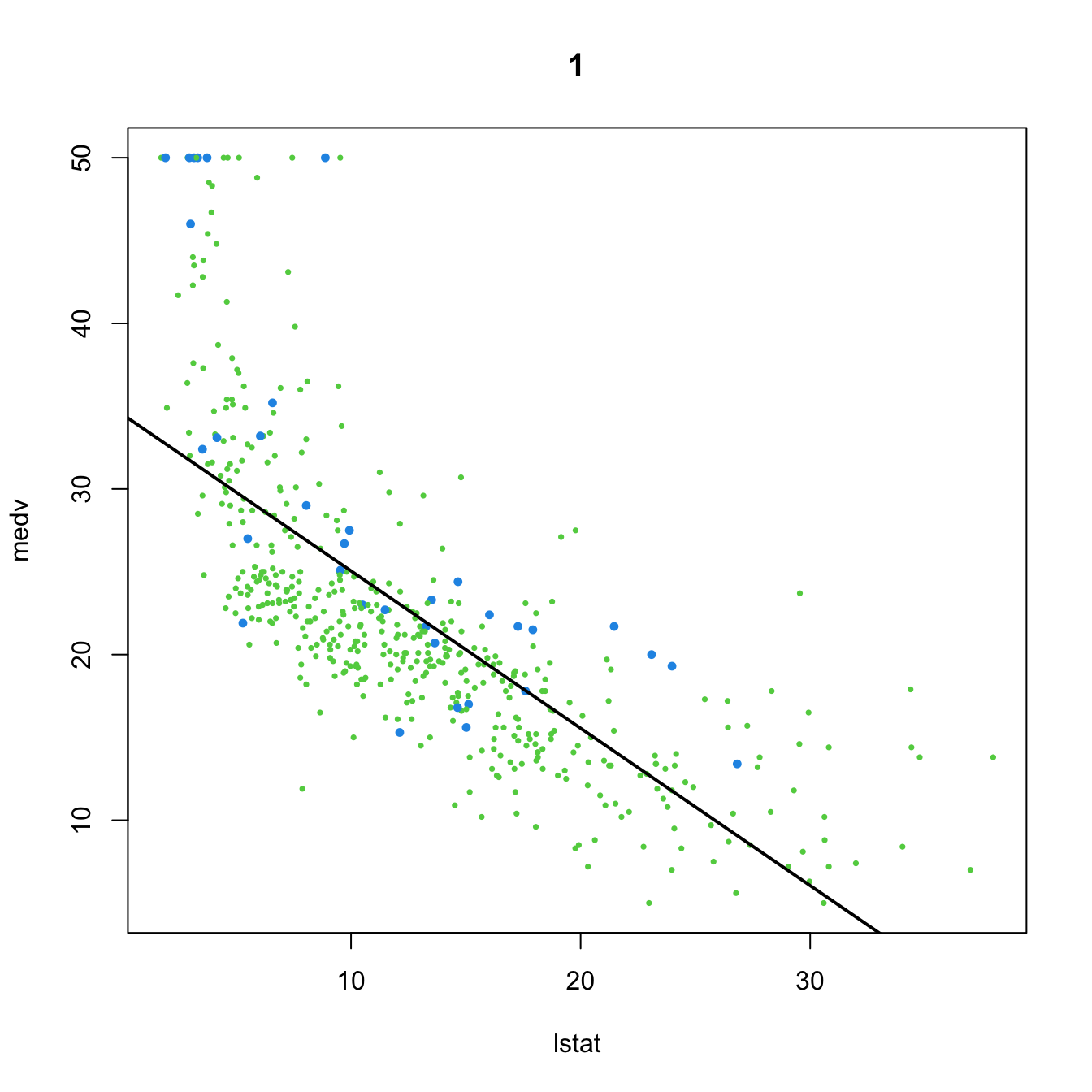

# 2. Dummy variable
(mod2 <- lm(medv ~ lstat + chas, data = Boston))
## 
## Call:
## lm(formula = medv ~ lstat + chas, data = Boston)
## 
## Coefficients:
## (Intercept)        lstat         chas  
##     34.0941      -0.9406       4.9200
plot(medv ~ lstat, data = Boston, col = col, pch = 16, cex = cex, main = "2")
abline(a = mod2$coefficients[1], b = mod2$coefficients[2], col = 3, lwd = 2)
abline(a = mod2$coefficients[1] + mod2$coefficients[3],
       b = mod2$coefficients[2], col = 4, lwd = 2)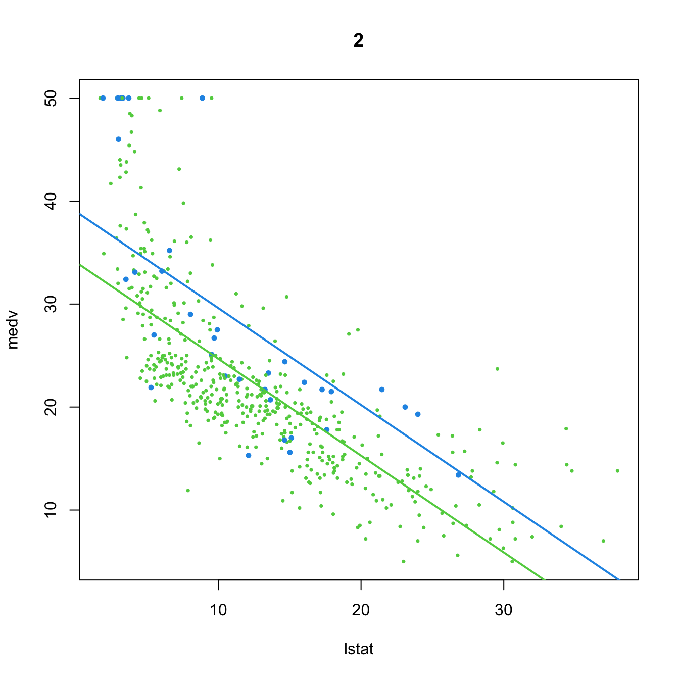

# 3. Dummy variable, with interaction
(mod3 <- lm(medv ~ lstat * chas, data = Boston))
## 
## Call:
## lm(formula = medv ~ lstat * chas, data = Boston)
## 
## Coefficients:
## (Intercept)        lstat         chas   lstat:chas  
##     33.7672      -0.9150       9.8251      -0.4329
plot(medv ~ lstat, data = Boston, col = col, pch = 16, cex = cex, main = "3")
abline(a = mod3$coefficients[1], b = mod3$coefficients[2], col = 3, lwd = 2)
abline(a = mod3$coefficients[1] + mod3$coefficients[3],
       b = mod3$coefficients[2] + mod3$coefficients[4], col = 4, lwd = 2)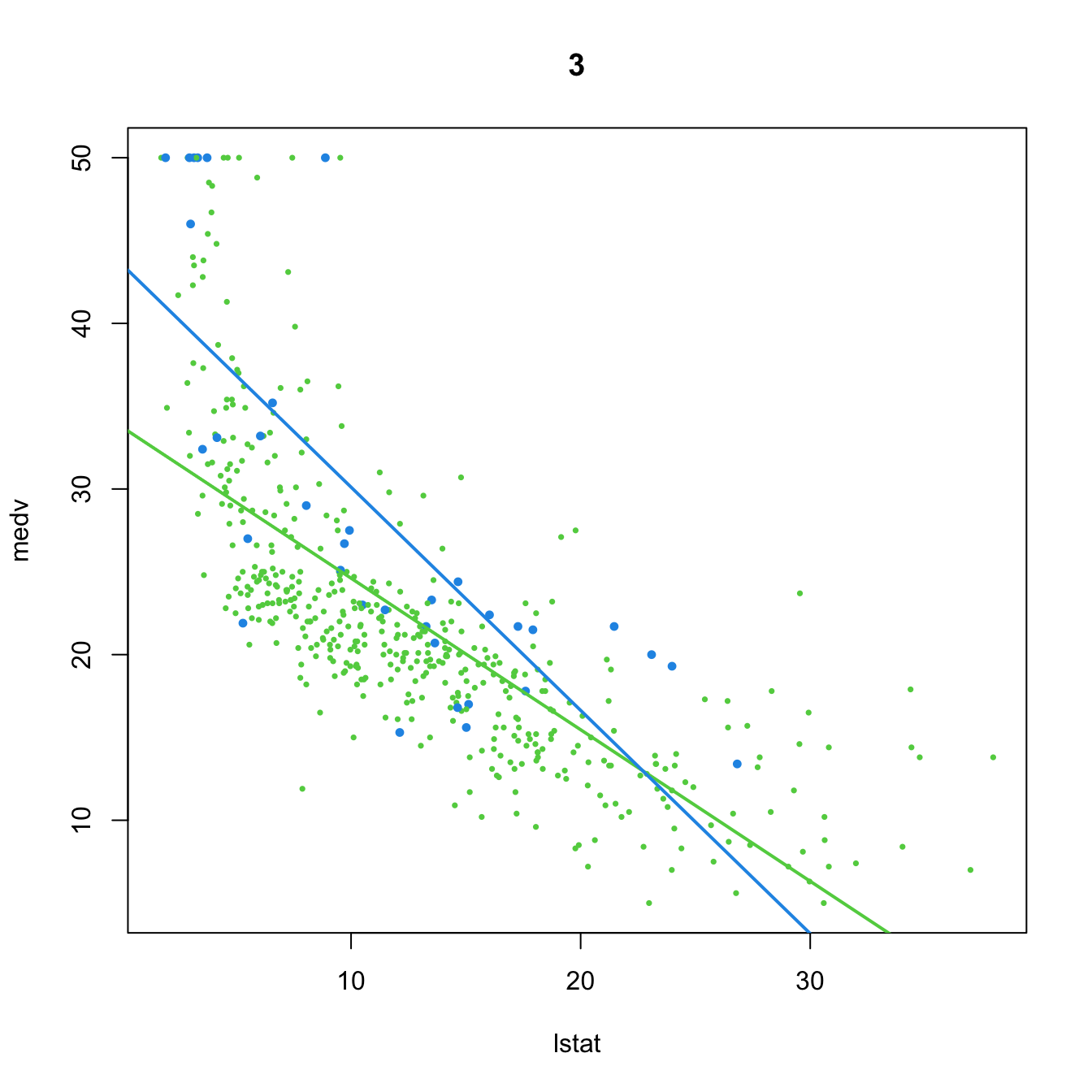

# 4. Dummy variable only present in interaction
(mod4 <- lm(medv ~ lstat + lstat:chas, data = Boston))
## 
## Call:
## lm(formula = medv ~ lstat + lstat:chas, data = Boston)
## 
## Coefficients:
## (Intercept)        lstat   lstat:chas  
##     34.4893      -0.9580       0.2128
plot(medv ~ lstat, data = Boston, col = col, pch = 16, cex = cex, main = "4")
abline(a = mod4$coefficients[1], b = mod4$coefficients[2], col = 3, lwd = 2)
abline(a = mod4$coefficients[1],
       b = mod4$coefficients[2] + mod4$coefficients[3], col = 4, lwd = 2)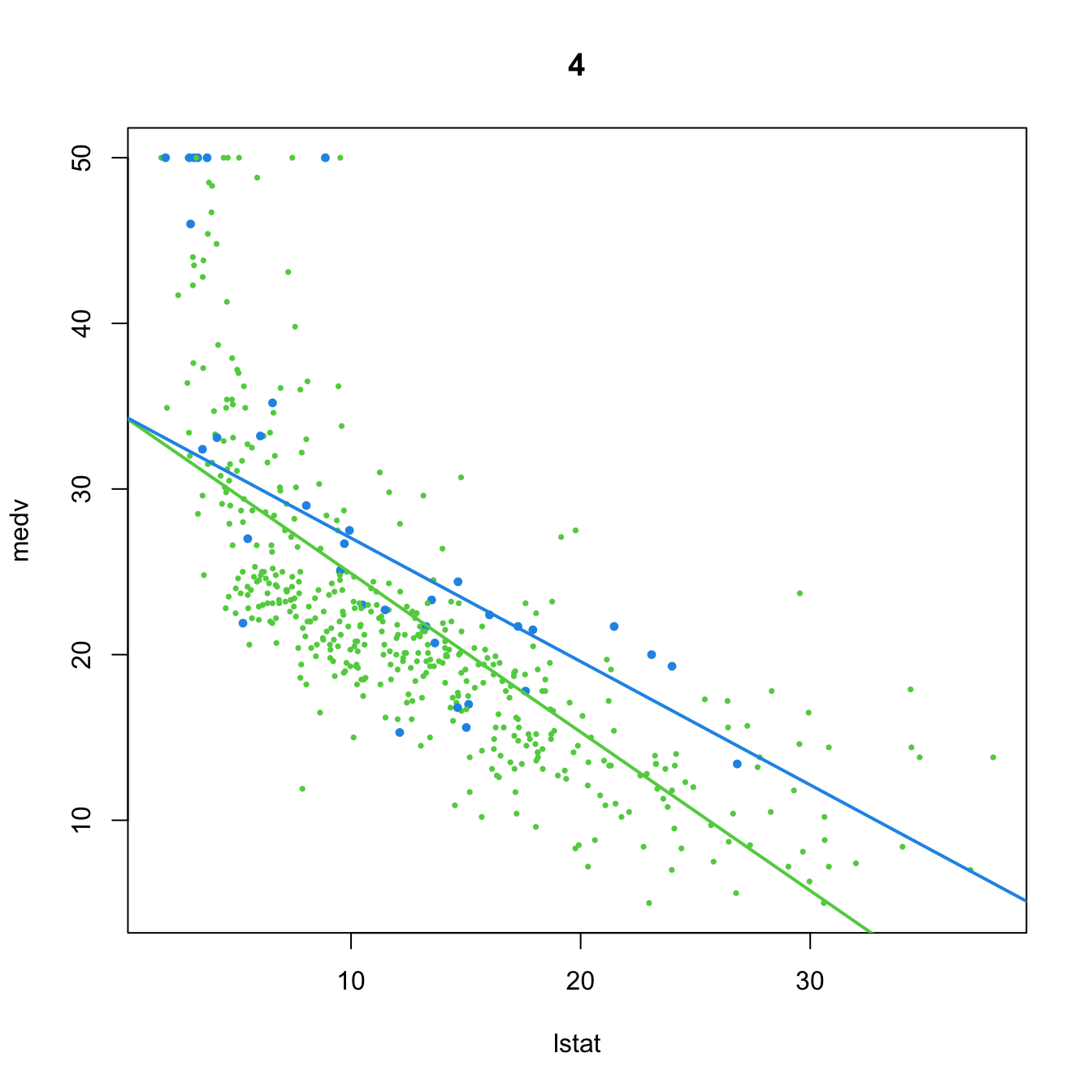

# 5. Dummy variable and no predictor
(mod5 <- lm(medv ~ chas, data = Boston))
## 
## Call:
## lm(formula = medv ~ chas, data = Boston)
## 
## Coefficients:
## (Intercept)         chas  
##      22.094        6.346
plot(medv ~ lstat, data = Boston, col = col, pch = 16, cex = cex, main = "5")
abline(a = mod5$coefficients[1], b = 0, col = 3, lwd = 2)
abline(a = mod5$coefficients[1] + mod5$coefficients[2], b = 0, col = 4, lwd = 2)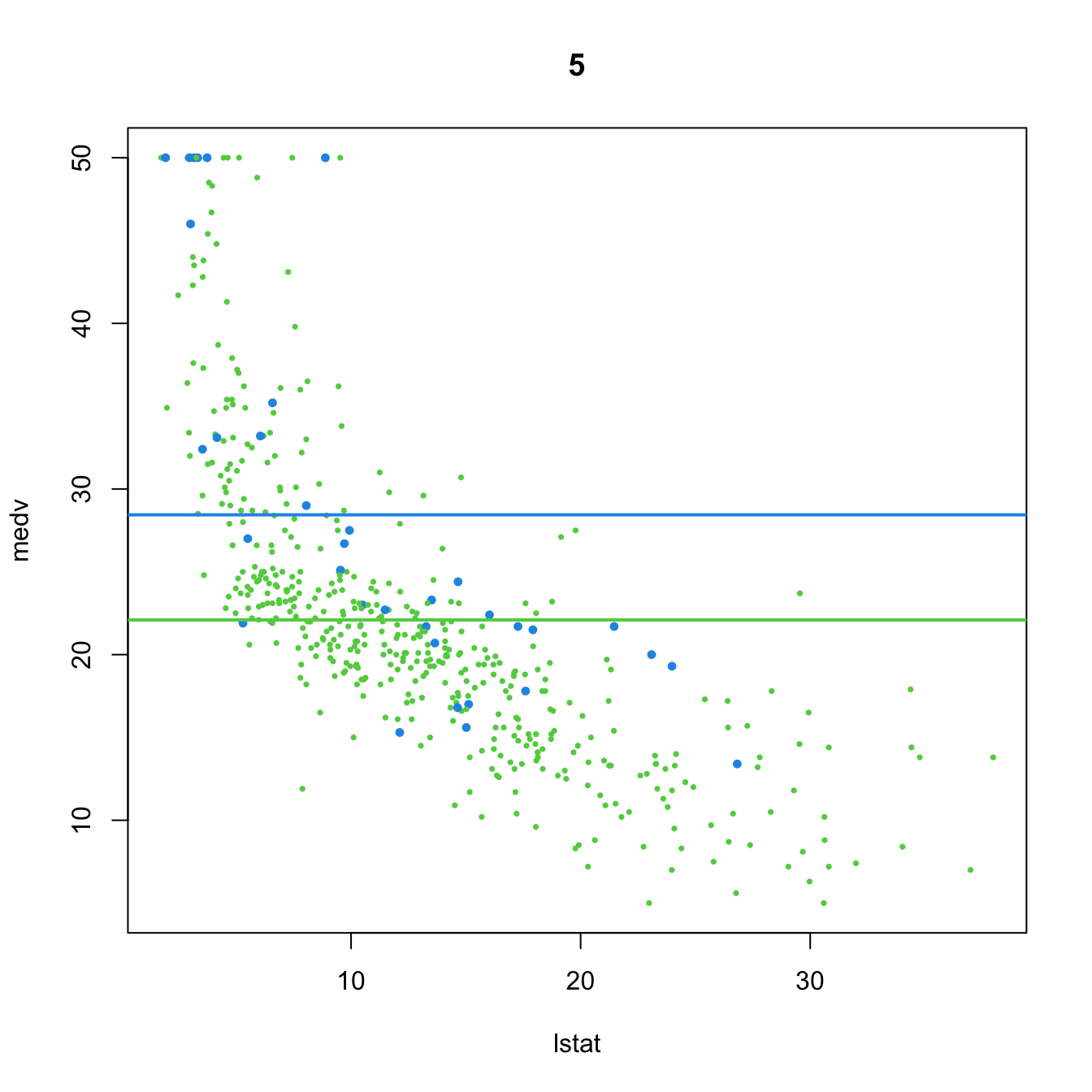

# 6. Dummy variable. Interaction in the intercept and slope
(mod6 <- lm(medv ~ chas + lstat:chas, data = Boston))
## 
## Call:
## lm(formula = medv ~ chas + lstat:chas, data = Boston)
## 
## Coefficients:
## (Intercept)         chas   chas:lstat  
##      22.094       21.498       -1.348
plot(medv ~ lstat, data = Boston, col = col, pch = 16, cex = cex, main = "6")
abline(a = mod6$coefficients[1], b = 0, col = 3, lwd = 2)
abline(a = mod6$coefficients[1] + mod6$coefficients[2],
       b = mod6$coefficients[3], col = 4, lwd = 2)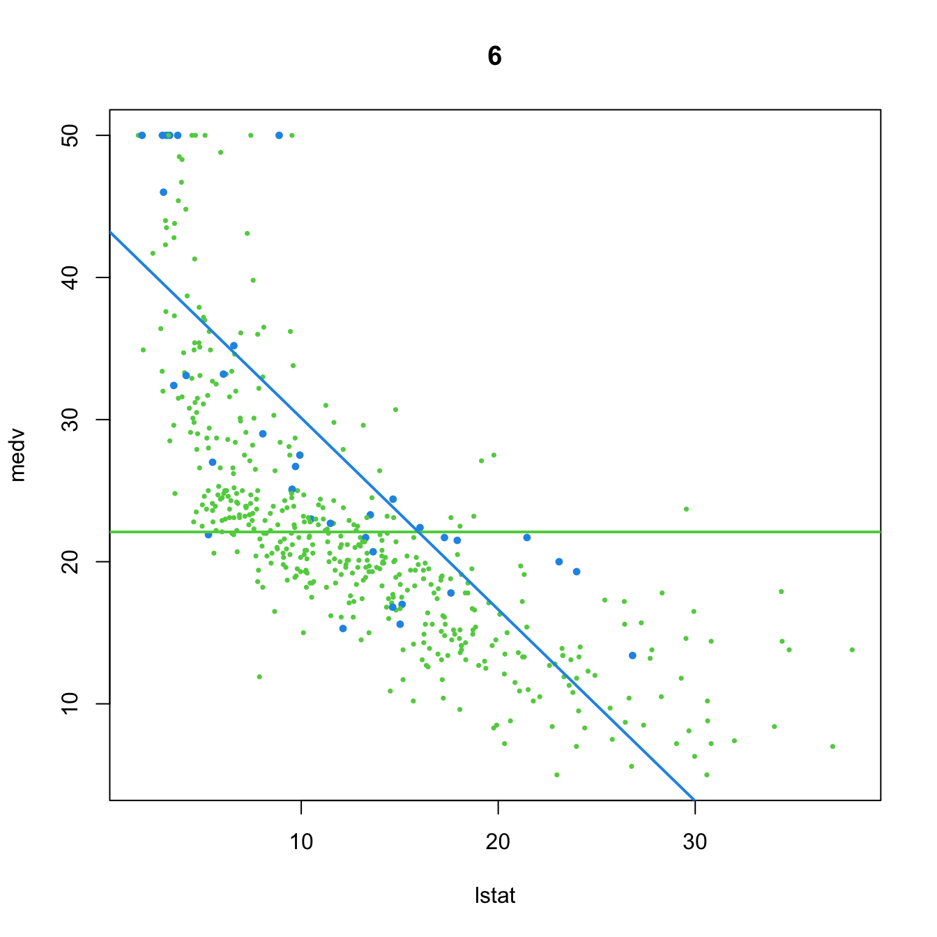

# 7. Dummy variable. Interaction in the slope
(mod7 <- lm(medv ~ lstat:chas, data = Boston))
## 
## Call:
## lm(formula = medv ~ lstat:chas, data = Boston)
## 
## Coefficients:
## (Intercept)   lstat:chas  
##    22.49484      0.04882
plot(medv ~ lstat, data = Boston, col = col, pch = 16, cex = cex, main = "7")
abline(a = mod7$coefficients[1], b = 0, col = 3, lwd = 2)
abline(a = mod7$coefficients[1], b = mod7$coefficients[2], col = 4, lwd = 2)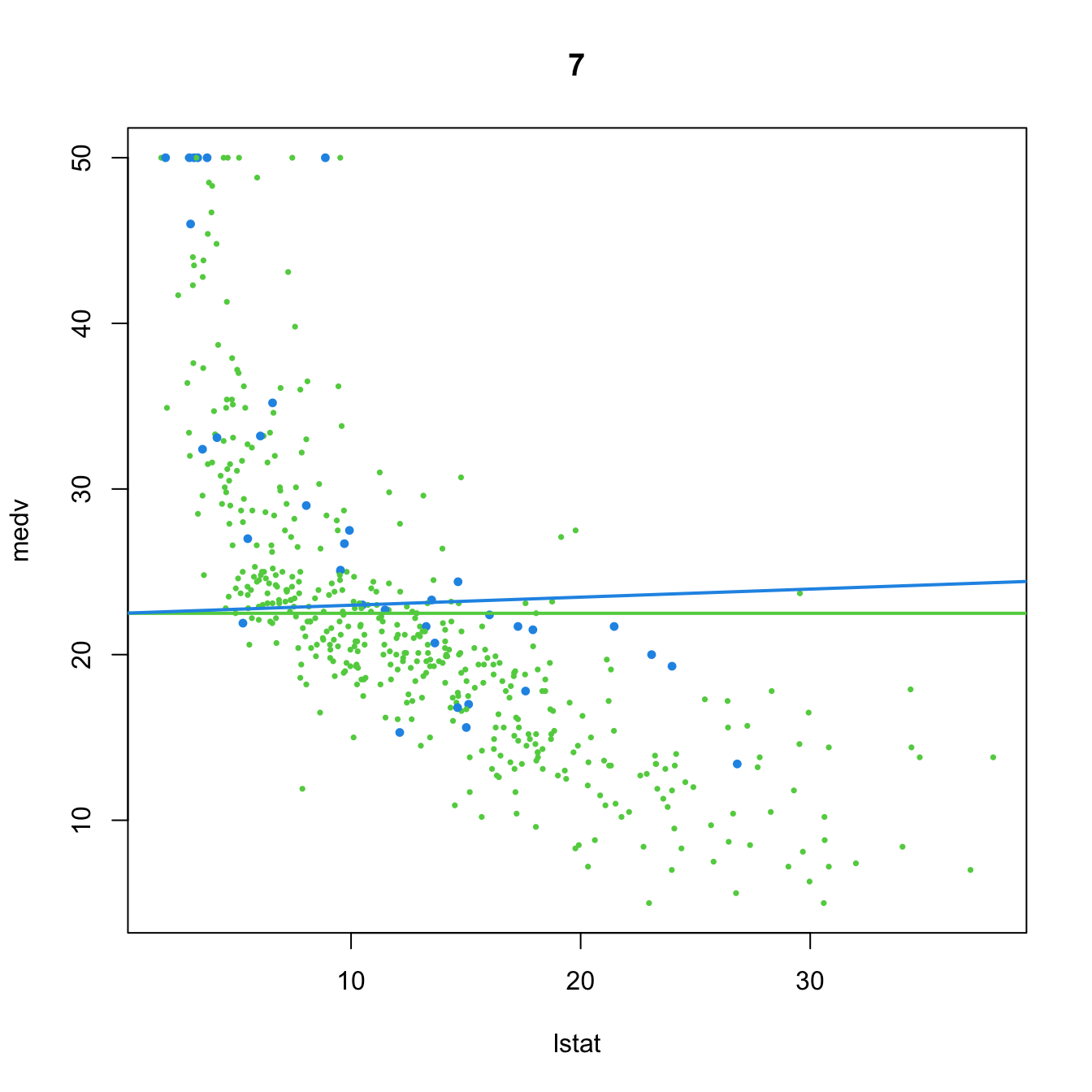

From the above illustration, it is clear that the effect of adding a dummy variable is to simultaneously fit two linear models (with varying flexibility) to the two groups of data encoded by the dummy variable, and merge this simultaneous fit within a single linear model. We can check this in more detail using the subset option of lm:

# Model using a dummy variable in the full dataset
lm(medv ~ lstat + chas + lstat:chas, data = Boston)
## 
## Call:
## lm(formula = medv ~ lstat + chas + lstat:chas, data = Boston)
## 
## Coefficients:
## (Intercept)        lstat         chas   lstat:chas  
##     33.7672      -0.9150       9.8251      -0.4329

# Individual model for the group with chas == 0
lm(medv ~ lstat, data = Boston, subset = chas == 0)
## 
## Call:
## lm(formula = medv ~ lstat, data = Boston, subset = chas == 0)
## 
## Coefficients:
## (Intercept)        lstat  
##      33.767       -0.915
# Notice that the intercept and lstat coefficient are the same as before

# Individual model for the group with chas == 1
lm(medv ~ lstat, data = Boston, subset = chas == 1)
## 
## Call:
## lm(formula = medv ~ lstat, data = Boston, subset = chas == 1)
## 
## Coefficients:
## (Intercept)        lstat  
##      43.592       -1.348
# Notice that the intercept and lstat coefficient equal the ones from the
# joint model, plus the specific terms associated with `chas`

This discussion can be extended to factors with several levels with more associated dummy variables. The next code chunk shows how three group-specific linear regressions are modeled together by means of two dummy variables in the iris dataset.

# Does not take into account the groups in the data
modIris <- lm(Sepal.Width ~ Petal.Width, data = iris)
modIris$coefficients
## (Intercept) Petal.Width 
##   3.3084256  -0.2093598

# Adding interactions with the groups
modIrisSpecies <- lm(Sepal.Width ~ Petal.Width * Species, data = iris)
modIrisSpecies$coefficients
##                   (Intercept)                   Petal.Width             Speciesversicolor              Speciesvirginica 
##                     3.2220507                     0.8371922                    -1.8491878                    -1.5272777 
## Petal.Width:Speciesversicolor  Petal.Width:Speciesvirginica 
##                     0.2164556                    -0.2057870

# Joint regression line shows negative correlation, but each group
# regression line shows a positive correlation
plot(Sepal.Width ~ Petal.Width, data = iris, col = as.integer(Species) + 1,
     pch = 16)
abline(a = modIris$coefficients[1], b = modIris$coefficients[2], lwd = 2)
abline(a = modIrisSpecies$coefficients[1], b = modIrisSpecies$coefficients[2],
       col = 2, lwd = 2)
abline(a = modIrisSpecies$coefficients[1] + modIrisSpecies$coefficients[3],
       b = modIrisSpecies$coefficients[2] + modIrisSpecies$coefficients[5],
       col = 3, lwd = 2)
abline(a = modIrisSpecies$coefficients[1] + modIrisSpecies$coefficients[4],
       b = modIrisSpecies$coefficients[2] + modIrisSpecies$coefficients[6],
       col = 4, lwd = 2)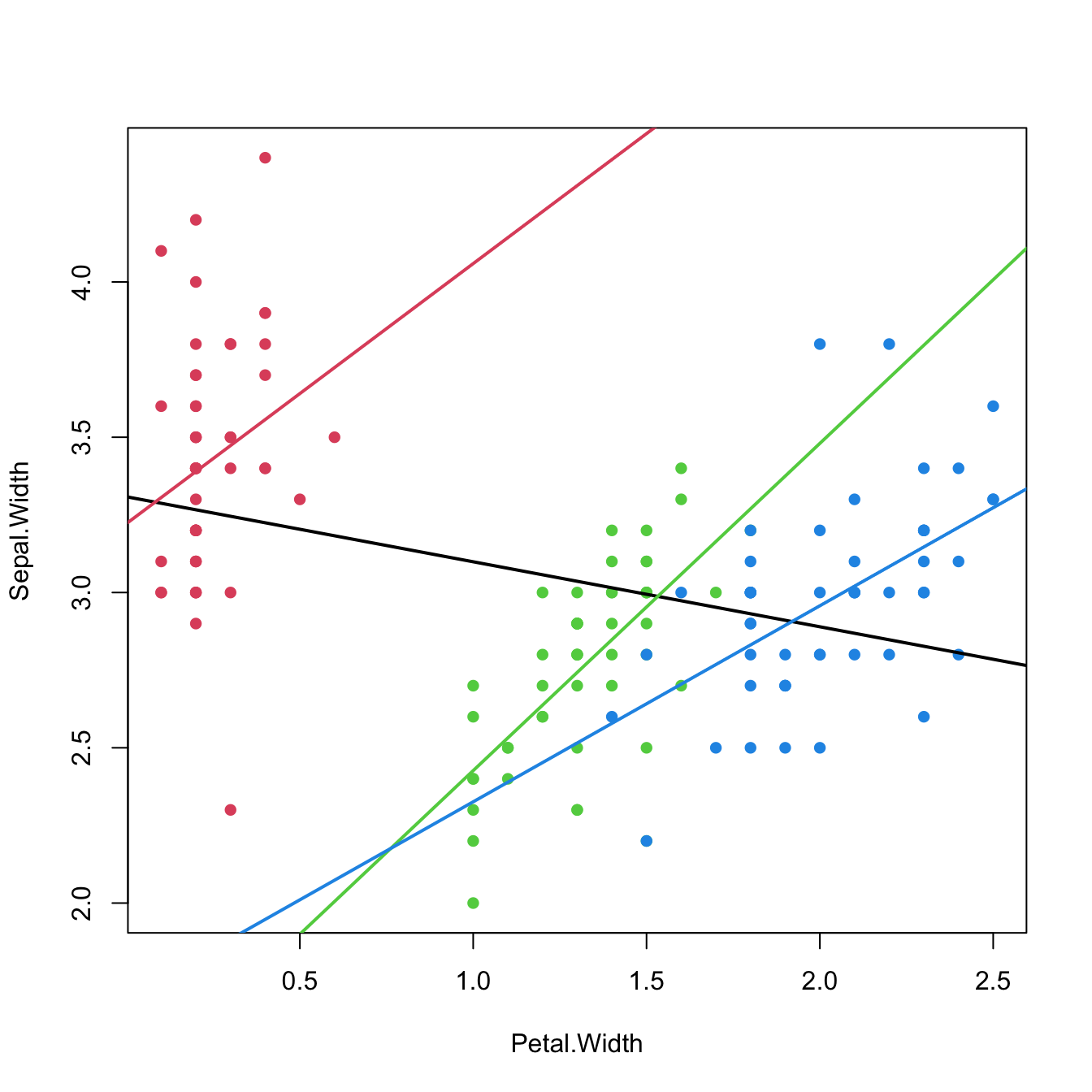

Figure 3.14: The three linear fits of Sepal.Width ~ Petal.Width * Species for each of the three levels in the Species factor (setosa in red, versicolor in green, and virginica in blue) in the iris dataset. The black line represents the linear fit for Sepal.Width ~ Petal.Width, that is, the linear fit without accounting for the levels in Species. Recall how Sepal.Width is positively correlated with Petal.Width within each group, but is negatively correlated in the aggregated data.

The last scatterplot is an illustration of the Simpson’s paradox. The simplest case of the paradox arises in simple linear regression, when there are two or more well-defined groups in the data such that:

1. Within each group, there is a clear and common correlation pattern between the response and the predictor.
2. When the groups are aggregated, the response and the predictor exhibit an opposite correlation pattern.

If groups are present in the data, always explore the intra-group correlations!

3.4.4 Case study application

The model employed in Harrison and Rubinfeld (1978) is different from the modBIC model. In the paper, several nonlinear transformations of the predictors and the response are done to improve the linear fit. Also, different units are used for medv, black, lstat, and nox. The authors considered these variables:

• Response: log(1000 * medv).
• Linear predictors: age, black / 1000 (this variable corresponds to their \((B-0.63)^2\)), tax, ptratio, crim, zn, indus, and chas.
• Nonlinear predictors: rm^2, log(dis), log(rad), log(lstat / 100), and (10 * nox)^2.

Exercise 3.8 Do the following:

1. Check if the model with such predictors corresponds to the one in the first column, Table VII, page 100 of Harrison and Rubinfeld (1978) (open-access paper available here). To do so, save this model as modelHarrison and summarize it.

2. Make a stepAIC selection of the variables in modelHarrison (use BIC) and save it as modelHarrisonSel. Summarize the fit.

3. Which model has a larger \(R^2\)? And \(R^2_\text{Adj}\)? Which is simpler and has more significant coefficients?

3.5 Model diagnostics

As we saw in Section 2.3, checking the assumptions of the multiple linear model through the visualization of the data becomes tricky even when \(p=2.\) To solve this issue, a series of diagnostic tools have been designed in order to evaluate graphically and systematically the validity of the assumptions of the linear model.

We will illustrate them in the wine dataset, which is available in the wine.RData workspace:

load("wine.RData")
mod <- lm(Price ~ Age + AGST + HarvestRain + WinterRain, data = wine)
summary(mod)

Before going into specifics, recall the following general comment on performing model diagnostics.

When one assumption fails, it is likely that this failure will affect other assumptions. For example, if linearity fails, then most likely homoscedasticity and normality will fail also. Therefore, identifying the root cause of the assumptions failure is key in order to try to find a patch.

3.5.1 Linearity

Linearity between the response \(Y\) and the predictors \(X_1,\ldots,X_p\) is the building block of the linear model. If this assumption fails, i.e., if there is a nonlinear trend linking \(Y\) and at least one of the predictors \(X_1,\ldots,X_p\) in a significant way, then the linear fit will yield flawed conclusions, with varying degrees of severity, about the explanation of \(Y.\) Therefore, linearity is a crucial assumption.

3.5.1.1 How to check it

The so-called residuals vs. fitted values plot is the scatterplot of \(\{(\hat Y_i,\hat\varepsilon_i)\}_{i=1}^n\) and is a very useful tool for detecting linearity departures using a single⁶⁹ graphical device. Figure 3.15 illustrates how the residuals vs. fitted values plots behave for situations in which the linearity is known to be respected or violated.

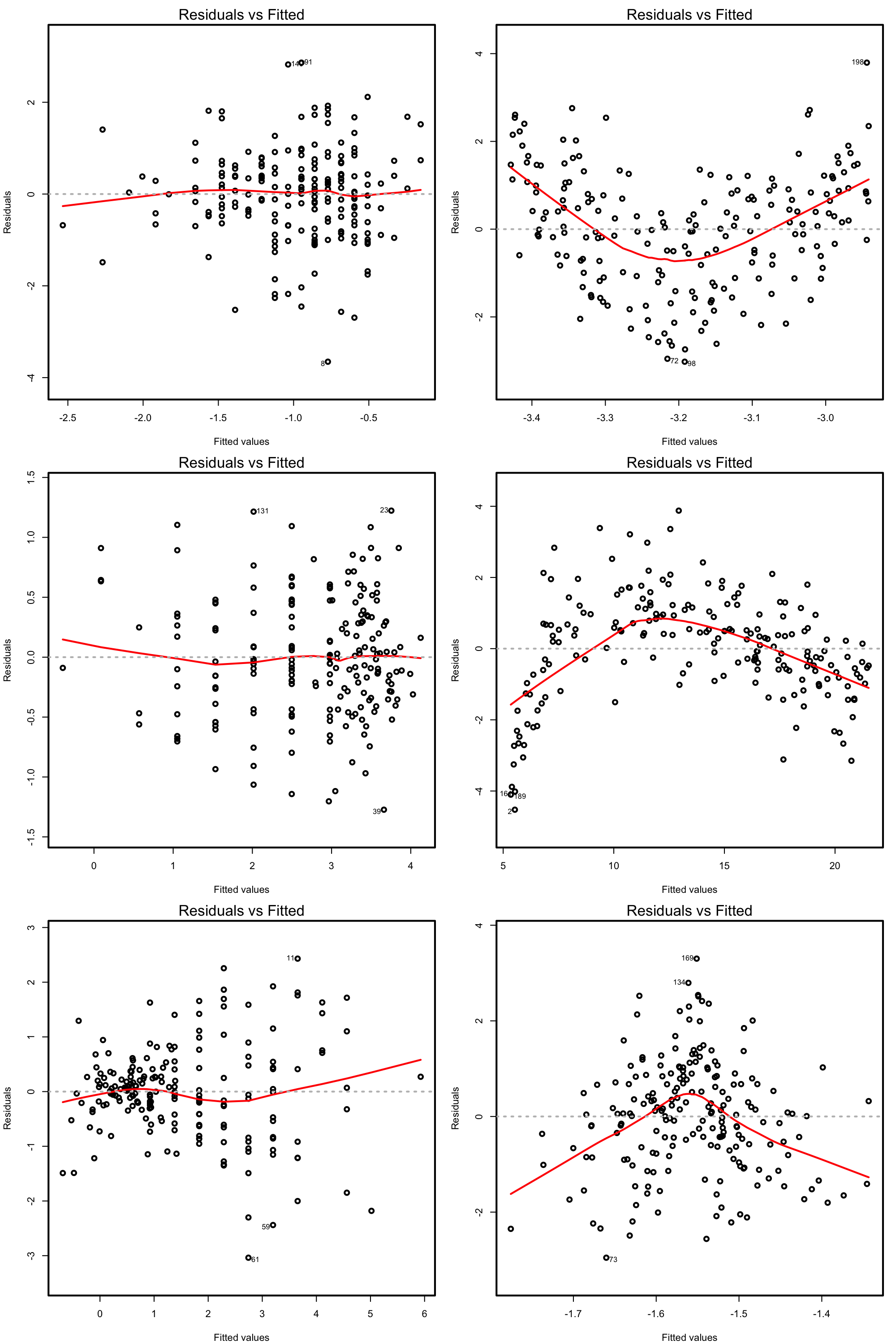
Figure 3.15: Residuals vs. fitted values plots for datasets respecting (left column) and violating (right column) the linearity assumption.

Under linearity, we expect that there is no significant trend in the residuals \(\hat\varepsilon_i\) with respect to \(\hat Y_i.\) This can be assessed by checking if a flexible fit of the mean of the residuals is constant. Such fit is given by the red line produced by:

plot(mod, 1)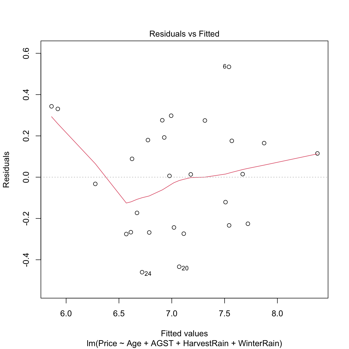

Figure 3.16: Residuals vs. fitted values for the Price ~ Age + AGST + HarvestRain + WinterRain model for the wine dataset.

If nonlinearities are observed, it is worth to plot the regression terms of the model. These are the \(p\) scatterplots of \(\{(X_{ij},Y_i)\}_{i=1}^n,\) for \(j=1,\ldots,p,\) that are accompanied by the regression lines \(y=\hat\beta_0+\hat\beta_jx_j,\) where \((\hat{\beta}_0,\hat{\beta}_1,\ldots,\hat{\beta}_p)^\top\) come from the multiple linear fit, not from individual simple linear regressions. The regression terms help identifying which predictors have nonlinear effects on \(Y.\)

par(mfrow = c(2, 2)) # We have 4 predictors
termplot(mod, partial.resid = TRUE)

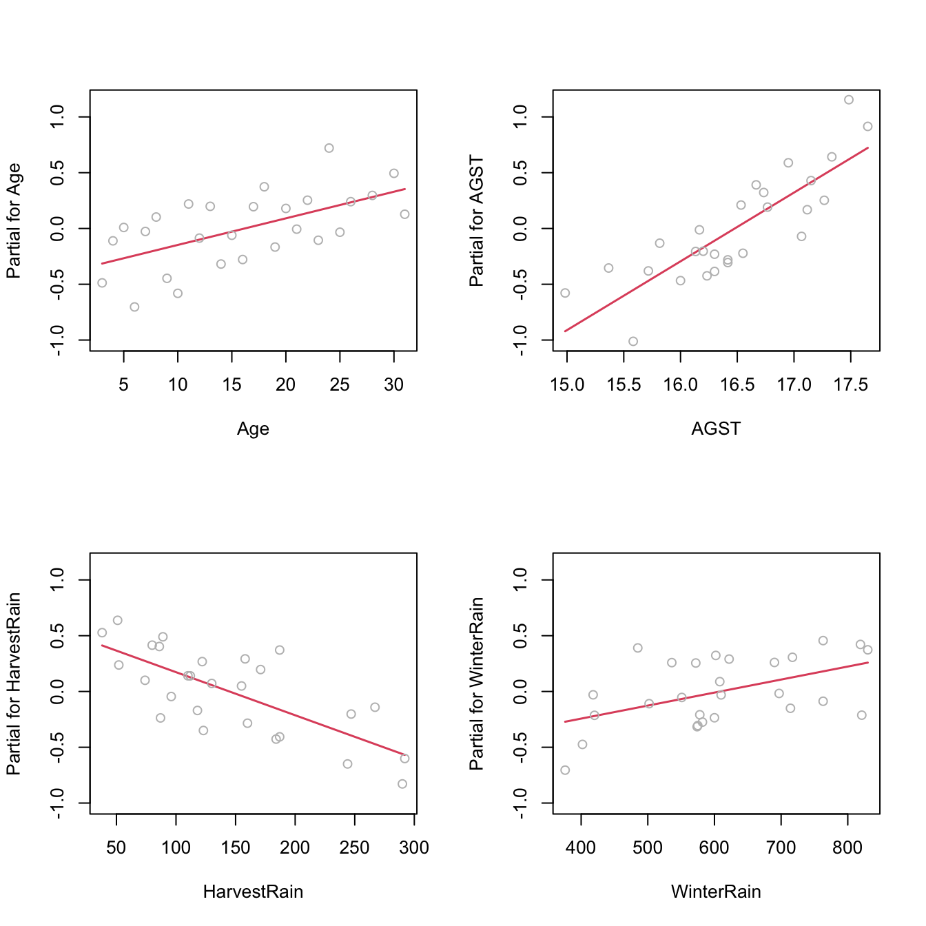
Figure 3.17: Regression terms for Price ~ Age + AGST + HarvestRain + WinterRain in the wine dataset.

3.5.1.2 What to do if it fails

Using an adequate nonlinear transformation for the problematic predictors or adding interaction terms, as we saw in Section 3.4, might be helpful in linearizing the relation between \(Y\) and \(X_1,\ldots,X_p.\) Alternatively, one can consider a nonlinear transformation \(f\) for the response \(Y,\) at the expenses of:

1. Modeling \(W:=f(Y)\) rather than \(Y,\) thus slightly changing the setting of the original modeling problem.
2. Alternatively, untransforming the linear prediction \(\hat{W}\) as \(\hat{Y}_f:=f^{-1}(\hat{W})\) and performing biased predictions⁷⁰ \(\!\!^,\)⁷¹ for \(Y.\)

Transformations of \(Y\) are explored in Section 3.5.7. Chapter 5 is devoted to replacing the untransformed approach with a more principled one.⁷²

Let’s see the transformation of predictors in the example that motivated Section 3.4.

par(mfrow = c(1, 2))
plot(lm(y ~ x, data = nonLinear), 1) # Nonlinear
plot(lm(y ~ I(x^2), data = nonLinear), 1) # Linear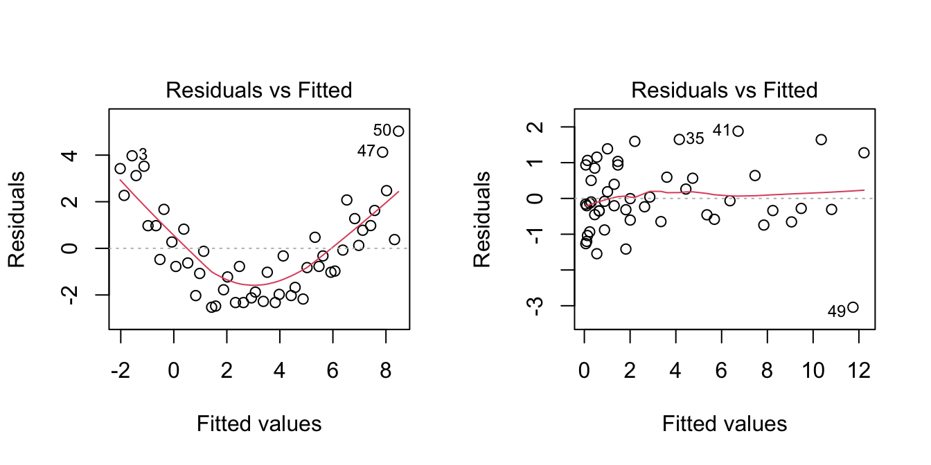

3.5.2 Normality

The assumed normality of the errors \(\varepsilon_1,\ldots,\varepsilon_n\) allows us to make exact inference in the linear model, in the sense that the distribution of \(\hat{\boldsymbol{\beta}}\) given in (2.11) is exact for any \(n,\) and not asymptotic with \(n\to\infty.\) If normality does not hold, then the inference we did (CIs for \(\beta_j,\) hypothesis testing, CIs for prediction) is to be somehow suspected. Why just somehow? Roughly speaking, the reason is that the central limit theorem will make \(\hat{\boldsymbol{\beta}}\) asymptotically normal⁷³, even if the errors are not. However, the speed of this asymptotic convergence greatly depends on how non-normal is the distribution of the errors. Hence the next rule of thumb:

Non-severe⁷⁴ departures from normality yield valid (asymptotic) inference for relatively large sample sizes \(n.\)

Therefore, the failure of normality is typically less problematic than other assumptions.

3.5.2.1 How to check it

The QQ-plot (theoretical quantile vs. empirical quantile plot) allows to check if the standardized residuals follow a \(\mathcal{N}(0,1).\) What it does is to compare the theoretical quantiles of a \(\mathcal{N}(0,1)\) with the quantiles of the sample of standardized residuals.

plot(mod, 2)

Figure 3.18: QQ-plot for the residuals of the Price ~ Age + AGST + HarvestRain + WinterRain model for the wine dataset.

Under normality, we expect the points to align with the diagonal line, which represents the expected position of the points if they were sampled from a \(\mathcal{N}(0,1).\) It is usual to have larger departures from the diagonal in the extremes⁷⁵ than in the center, even under normality, although these departures are more evident if the data is non-normal.

There are formal tests to check the null hypothesis of normality in our residuals. Two popular ones are the Shapiro–Wilk test, implemented by the shapiro.test function, and the Lilliefors test,⁷⁶ implemented by the nortest::lillie.test function:

# Shapiro-Wilk test of normality
shapiro.test(mod$residuals)
## 
##  Shapiro-Wilk normality test
## 
## data:  mod$residuals
## W = 0.95903, p-value = 0.3512
# We do not reject normality
# shapiro.test allows up to 5000 observations -- if dealing with more data
# points, randomization of the input is a possibility

# Lilliefors test -- the Kolmogorov-Smirnov adaptation for testing normality
nortest::lillie.test(mod$residuals)
## 
##  Lilliefors (Kolmogorov-Smirnov) normality test
## 
## data:  mod$residuals
## D = 0.13739, p-value = 0.2125
# We do not reject normality

Figure 3.19: QQ-plots for datasets respecting (left column) and violating (right column) the normality assumption.

Figure 3.20: The uncertainty behind the QQ-plot. The figure aggregates \(M=1000\) different QQ-plots of \(\mathcal{N}(0,1)\) data with \(n=100,\) displaying for each of them the pairs \((x_p,\hat x_p)\) evaluated at \(p=\frac{i-1/2}{n},\) \(i=1,\ldots,n\) (as they result from ppoints(n)). The uncertainty is measured by the asymptotic \(100(1-\alpha)\%\) CIs for \(\hat x_p,\) given by \(\left(x_p\pm\frac{z_{1-\alpha/2}}{\sqrt{n}}\frac{\sqrt{p(1-p)}}{\phi(x_p)}\right).\) These curves are displayed in red for \(\alpha=0.05.\) Observe that the vertical strips arise since the \(x_p\) coordinate is deterministic.

3.5.2.2 What to do if it fails

Patching non-normality is not easy and most of the time requires the consideration of other models, like the ones seen in Chapter 5. If \(Y\) is nonnegative, one possibility is to transform \(Y\) by means of the Box–Cox (Box and Cox 1964) transformation:

\[\begin{align} y^{(\lambda)}:=\begin{cases} \frac{y^\lambda-1}{\lambda},& \lambda\neq0,\\ \log(y),& \lambda=0. \end{cases}\tag{3.6} \end{align}\]

This transformation alleviates the skewness⁷⁷ of the data, therefore making it more symmetric and hence normal-like. The optimal data-dependent \(\hat\lambda\) that makes the data most normal-like can be found through maximum likelihood⁷⁸ on the transformed sample \(\{Y^{(\lambda)}_{i}\}_{i=1}^n.\) If \(Y\) is not nonnegative, (3.6) cannot be applied. A possible patch is to shift the data by a positive constant \(m=-\min(Y_1,\ldots,Y_n)+\delta,\) \(\delta>0,\) such that transformation (3.6) becomes

\[\begin{align*} y^{(\lambda,m)}:=\begin{cases} \frac{(y+m)^\lambda-1}{\lambda},& \lambda\neq0,\\ \log(y+m),& \lambda=0. \end{cases} \end{align*}\]

A neat alternative to this shifting is to rely on a transformation that is already designed for real \(Y,\) such as the Yeo–Johnson (Yeo and Johnson 2000) transformation:

\[\begin{align} y^{(\lambda)}:=\begin{cases} \frac{(y+1)^\lambda-1}{\lambda},& \lambda\neq0,y\geq 0,\\ \log(y+1),& \lambda=0,y\geq 0,\\ -\frac{(-y+1)^{2-\lambda}-1}{2-\lambda},& \lambda\neq2,y<0,\\ -\log(-y+1),& \lambda=2,y<0. \end{cases}\tag{3.7} \end{align}\]

The beauty of the Yeo–Johnson transformation is that it extends neatly the Box–Cox transformation, which appears as a particular case when \(Y\) is nonnegative and after performing a shift of \(1\) unit (see Figure 3.21). As with the Box–Cox transformation, the optimal \(\hat\lambda\) is estimated through maximum likelihood on the transformed sample \(\{Y^{(\lambda)}_{i}\}_{i=1}^n.\)

N <- 200
y <- seq(-4, 4, length.out = N)
lambda <- c(0, 0.5, 1, 2, -0.5, -1, -2)
l <- length(lambda)
psi <- sapply(lambda, function(la) car::yjPower(U = y, lambda = la))
matplot(y, psi, type = "l", ylim = c(-4, 4), lwd = 2, lty = 1:l,
        ylab = latex2exp::TeX("$y^{(\\lambda)}$"), col = 1:l, las = 1,
        main = "Yeo-Johnson transformation")
abline(v = 0, h = 0)
abline(v = -1, h = 0, lty = 2)
legend("bottomright", lty = 1:l, lwd = 2, col = 1:l,
       legend = latex2exp::TeX(paste0("$\\lambda = ", lambda, "$")))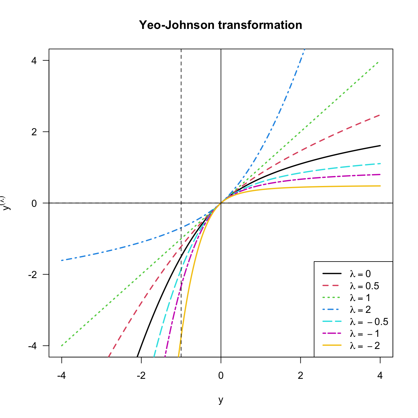

Figure 3.21: Yeo–Johnson transformation for some values of \(\lambda.\) The Box–Cox transformation for \(\lambda,\) and shifted by \(-1\) units, corresponds to the part \(y\geq -1\) of the plot.

Let’s see how to implement both transformations using the car::powerTransform, car::bcPower, and car::yjPower functions.

# Test data

# Predictors
n <- 200
set.seed(121938)
X1 <- rexp(n, rate = 1 / 5) # Nonnegative
X2 <- rchisq(n, df = 5) - 3 # Real

# Response of a linear model
epsilon <- rchisq(n, df = 10) - 10 # Centered error, but not normal
Y <- 10 - 0.5 * X1 + X2 + epsilon

# Transformation of non-normal data to achieve normal-like data (no model)

# Optimal lambda for Box-Cox
BC <- car::powerTransform(lm(X1 ~ 1), family = "bcPower") # Maximum-likelihood fit
# Note we use a regression model with no predictors
(lambdaBC <- BC$lambda) # The optimal lambda
##        Y1 
## 0.2412419
# lambda < 1, so positive skewness is corrected

# Box-Cox transformation
X1Transf <- car::bcPower(U = X1, lambda = lambdaBC)

# Comparison
par(mfrow = c(1, 2))
hist(X1, freq = FALSE, breaks = 10, ylim = c(0, 0.3))
hist(X1Transf, freq = FALSE, breaks = 10, ylim = c(0, 0.3))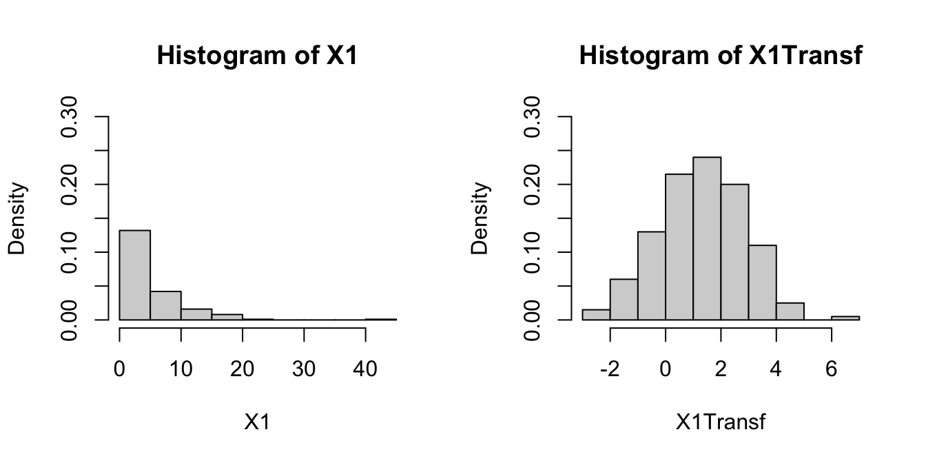

# Optimal lambda for Yeo-Johnson
YJ <- car::powerTransform(lm(X2 ~ 1), family = "yjPower")
(lambdaYJ <- YJ$lambda)
##        Y1 
## 0.5850791

# Yeo-Johnson transformation
X2Transf <- car::yjPower(U = X2, lambda = lambdaYJ)

# Comparison
par(mfrow = c(1, 2))
hist(X2, freq = FALSE, breaks = 10, ylim = c(0, 0.3))
hist(X2Transf, freq = FALSE, breaks = 10, ylim = c(0, 0.3))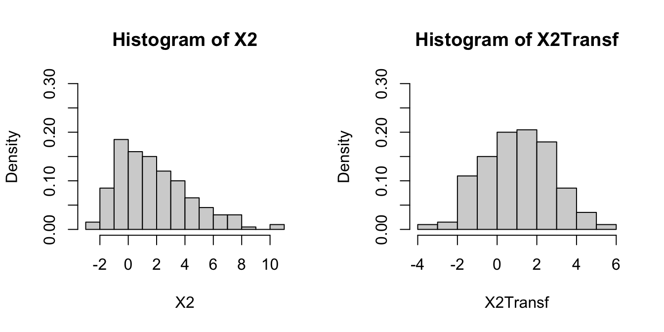

# Transformation of non-normal response in a linear model

# Optimal lambda for Yeo-Johnson
YJ <- car::powerTransform(lm(Y ~ X1 + X2), family = "yjPower")
(lambdaYJ <- YJ$lambda)
##        Y1 
## 0.9160924

# Yeo-Johnson transformation
YTransf <- car::yjPower(U = Y, lambda = lambdaYJ)

# Comparison for the residuals
par(mfrow = c(1, 2))
plot(lm(Y ~ X1 + X2), 2)
plot(lm(YTransf ~ X1 + X2), 2) # Slightly better

Be aware that using the previous transformations implies modeling the transformed response rather than \(Y.\) Normality is also possible to patch if it is a consequence of the failure of linearity or homoscedasticity, which translates the problem into fixing those assumptions.

3.5.3 Homoscedasticity

The constant-variance assumption of the errors is also key for obtaining the inferential results we saw. For example, if the assumption does not hold, then the CIs for prediction will not respect the confidence for which they were built.

3.5.3.1 How to check it

Heteroscedasticity can be detected by looking into irregular vertical dispersion patterns in the residuals vs. fitted values plot. However, it is simpler to use the scale-location plot, where the standardized residuals are transformed by a square root of its absolute value, and inspect the deviations in the positive axis.

plot(mod, 3)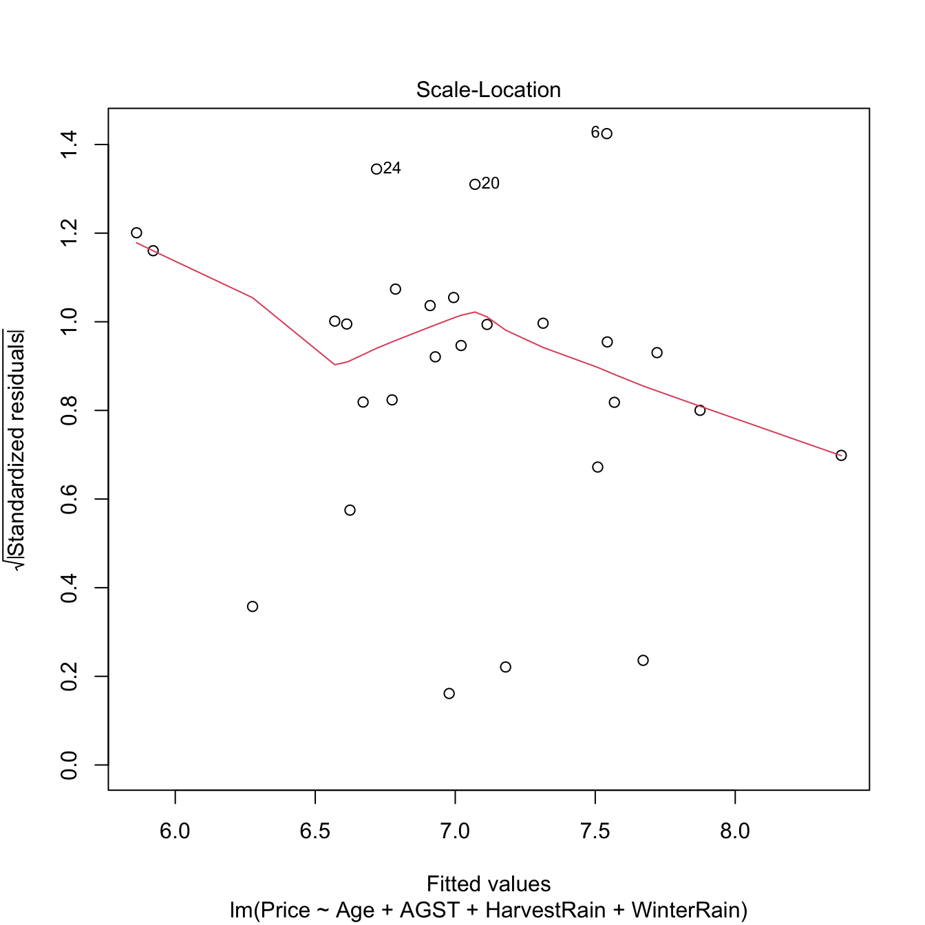

Figure 3.22: Scale-location plot for the Price ~ Age + AGST + HarvestRain + WinterRain model for the wine dataset.

Under homoscedasticity, we expect the red line, a flexible fit of the mean of the transformed residuals, to be almost constant about \(1\). If there are clear non-constant patterns, then there is evidence of heteroscedasticity.

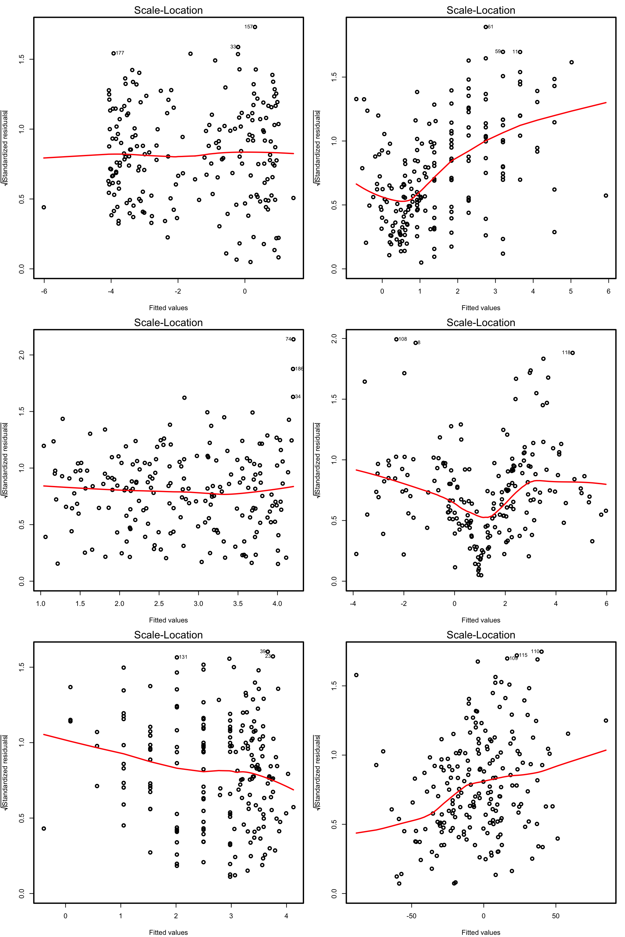
Figure 3.23: Scale-location plots for datasets respecting (left column) and violating (right column) the homoscedasticity assumption.

There are formal tests to check the null hypothesis of homoscedasticity in our residuals. For example, the Breusch–Pagan test implemented in car::ncvTest:

# Breusch-Pagan test
car::ncvTest(mod)
## Non-constant Variance Score Test 
## Variance formula: ~ fitted.values 
## Chisquare = 0.3254683, Df = 1, p = 0.56834
# We do not reject homoscedasticity

The Breusch–Pagan test checks homoscedasticity against a non-constant variance in the residuals that is linearly increasing with respect to the predictors. This means that the test can be fooled by a nonlinear pattern in the variance of the residuals that results in a flat linear fit (e.g., a quadratic pattern). It is advised then to check the scale-location plot if performing the Breusch–Pagan test, in order to identify evident non-constant variances hidden behind tricky nonlinearities.

The next code illustrates the previous warning with two examples.

# Heteroscedastic models
set.seed(123456)
x <- rnorm(100)
y1 <- 1 + 2 * x + rnorm(100, sd = x^2)
y2 <- 1 + 2 * x + rnorm(100, sd = 1 + x * (x > 0))
modHet1 <- lm(y1 ~ x)
modHet2 <- lm(y2 ~ x)

# Heteroscedasticity not detected
car::ncvTest(modHet1)
## Non-constant Variance Score Test 
## Variance formula: ~ fitted.values 
## Chisquare = 2.938652e-05, Df = 1, p = 0.99567
plot(modHet1, 3)

# Heteroscedasticity correctly detected
car::ncvTest(modHet2)
## Non-constant Variance Score Test 
## Variance formula: ~ fitted.values 
## Chisquare = 41.03562, Df = 1, p = 1.4948e-10
plot(modHet2, 3)

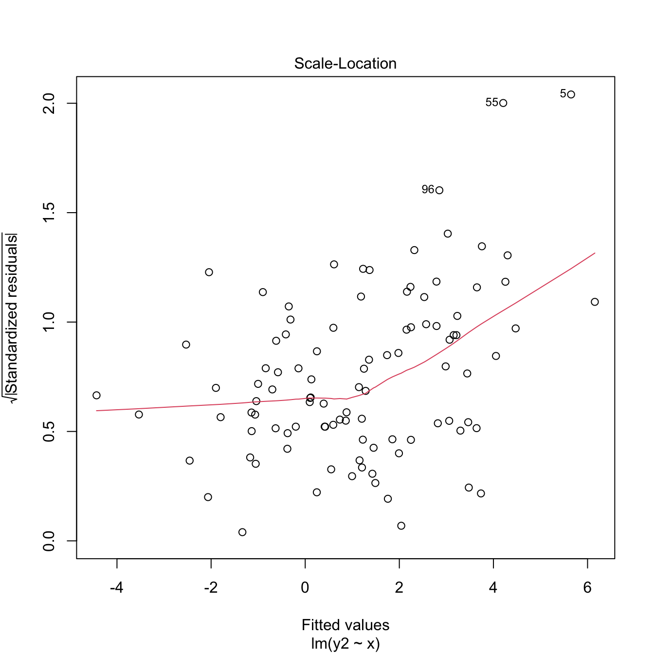
Figure 3.24: Two heteroscedasticity patterns that are undetected and detected, respectively, by the Breusch–Pagan test.

3.5.3.2 What to do if it fails

Using a nonlinear transformation for the response \(Y\) may help to control the variance. Typical choices are \(\log(Y)\) and \(\sqrt{Y},\) which reduce the scale of the larger responses and leads to a reduction of heteroscedasticity. Keep in mind that these transformations, as the Box–Cox transformations, are designed for nonnegative \(Y.\) The Yeo–Johnson transformation can be used instead if \(Y\) is real.

Let’s see some examples.

# Artificial data with heteroscedasticity
set.seed(12345)
X <- rchisq(500, df = 3)
e <- rnorm(500, sd = sqrt(0.1 + 2 * X))
Y <- 1 + X + e

# Original
plot(lm(Y ~ X), 3) # Very heteroscedastic

# Transformed
plot(lm(I(log(abs(Y))) ~ X), 3) # Much less heteroscedastic, but at the price
# of losing the signs in Y...

# Shifted and transformed
delta <- 1 # This is tunable
m <- -min(Y) + delta
plot(lm(I(log(Y + m)) ~ X), 3) # No signs loss

# Transformed by Yeo-Johnson

# Optimal lambda for Yeo-Johnson
YJ <- car::powerTransform(lm(Y ~ X), family = "yjPower")
(lambdaYJ <- YJ$lambda)
##        Y1 
## 0.6932053

# Yeo-Johnson transformation
YTransf <- car::yjPower(U = Y, lambda = lambdaYJ)
plot(lm(YTransf ~ X), 3) # Slightly less heteroscedastic

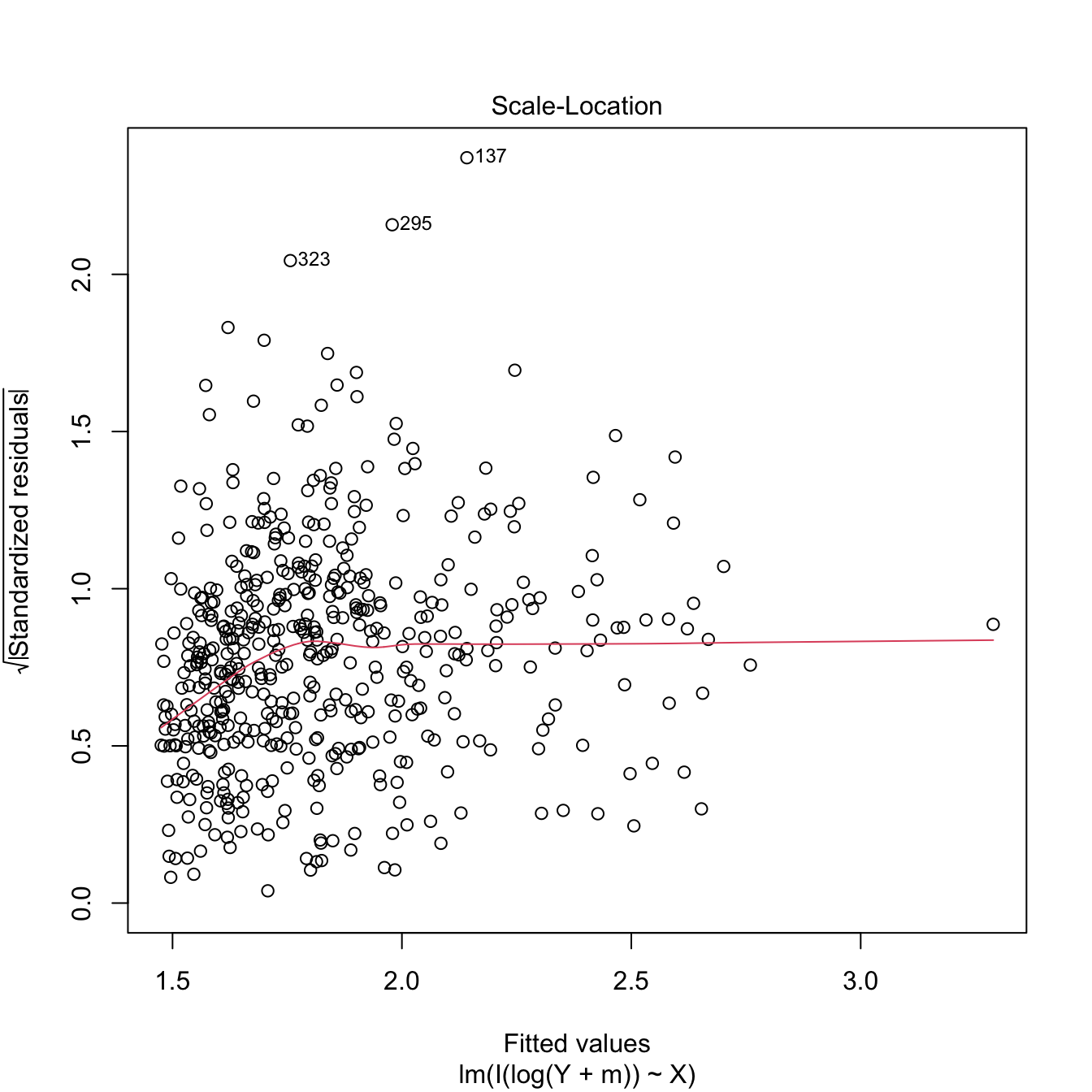
Figure 3.25: Patching of heteroscedasticity for an artificial dataset.

3.5.4 Independence

Independence is also a key assumption: it guarantees that the amount of information that we have on the relationship between \(Y\) and \(X_1,\ldots,X_p,\) from \(n\) observations, is maximal. If there is dependence, then information is repeated, and as a consequence the variability of the estimates will be larger. For example, \(95\%\) CIs built under the assumption of independence will be shorter than the adequate, meaning that they will not contain with a \(95\%\) confidence the unknown parameter, but with a lower confidence (say \(80\%\)).

An extreme case is the following: suppose we have two samples of sizes \(n\) and \(2n,\) where the \(2n\)-sample contains the elements of the \(n\)-sample twice. The information in both samples is the same, and so are the estimates for the coefficients \(\boldsymbol{\beta}.\) Yet, in the \(2n\)-sample the length of the confidence intervals is \(C(2n)^{-1/2},\) whereas in the \(n\)-sample they have length \(Cn^{-1/2}.\) A reduction by a factor of \(\sqrt{2}\) in the confidence interval has happened, but we have the same information! This will give us a wrong sense of confidence in our model, and the root of the evil is that the information that is actually in the sample is smaller due to dependence.

3.5.4.1 How to check it

The set of possible dependence structures on the residuals is immense, and there is no straightforward way of checking all of them. Usually what it is examined is the presence of autocorrelation, which appears when there is some kind of serial dependence in the measurement of observations. The serial plot of the residuals allows to detect time trends in them:

plot(mod$residuals, type = "o")

Figure 3.26: Serial plot of the residuals of the Price ~ Age + AGST + HarvestRain + WinterRain model for the wine dataset.

Under uncorrelation, we expect the series to show no tracking of the residuals. That is, that the closer observations do not take similar values, but rather change without any kind of distinguishable pattern. Tracking is associated to positive autocorrelation, but negative autocorrelation, manifested as alternating small-large or positive-negative residuals, is also possible. The lagged plots of \((\hat\varepsilon_{i-\ell},\hat\varepsilon_i),\) \(i=\ell+1,\ldots,n,\) obtained through lag.plot, allow us to detect both kinds of autocorrelations for a given lag \(\ell.\) Under independence, we expect no trend in such plot. Here is an example:

lag.plot(mod$residuals, lags = 1, do.lines = FALSE)

# No serious serial trend, but some negative autocorrelation is appreciated
cor(mod$residuals[-1], mod$residuals[-length(mod$residuals)])
## [1] -0.4267776

There are also formal tests for testing for the absence of autocorrelation, such as the Durbin–Watson test implemented in car::durbinWatsonTest:

# Durbin-Watson test
car::durbinWatsonTest(mod)
##  lag Autocorrelation D-W Statistic p-value
##    1      -0.4160168      2.787261   0.054
##  Alternative hypothesis: rho != 0
# Does not reject at alpha = 0.05

Figure 3.27: Serial plots of the residuals for datasets respecting (left column) and violating (right column) the independence assumption.

3.5.4.2 What to do if it fails

Little can be done if there is dependence in the data, once this has been collected. If the dependence is temporal, we must rely on the family of statistical models meant to deal with serial dependence: time series. Other kinds of dependence such as spatial dependence, spatio-temporal dependence, geometrically-driven dependencies, censorship, truncation, etc. need to be analyzed with a different set of tools to the ones covered in these notes.

However, there is a simple trick worth mentioning to deal with serial dependence. If the observations of the response \(Y,\) say \(Y_1,Y_2,\ldots,Y_n,\) present serial dependence, a differentiation of the sample that yields \(Y_1-Y_2,Y_2-Y_3,\ldots,Y_{n-1}-Y_n\) may lead to independent observations. These are called the innovations of the series of \(Y.\)

Exercise 3.9 Load the dataset assumptions3D.RData and compute the regressions y.3 ~ x1.3 + x2.3, y.4 ~ x1.4 + x2.4, y.5 ~ x1.5 + x2.5, and y.8 ~ x1.8 + x2.8. Use the presented diagnostic tools to test the assumptions of the linear model and look out for possible problems.

3.5.5 Multicollinearity

A common problem that arises in multiple linear regression is multicollinearity. This is the situation when two or more predictors are highly linearly related between them. Multicollinearity has important effects on the fit of the model:

• It reduces the precision of the estimates. As a consequence, the signs of fitted coefficients may be even reversed and valuable predictors may appear as non-significant. In limit cases, numerical instabilities may appear since \(\mathbf{X}^\top\mathbf{X}\) will be almost singular.
• It is difficult to determine how each of the highly-related predictors affects the response, since one masks the other.

Intuitively, multicollinearity can be visualized as a card (fitting plane) that is held on its opposite corners and that spins on its diagonal, where the data is concentrated. Then, very different planes will fit the data almost equally well, which results in a large variability of the optimal plane.

An approach to detect multicollinearity is to inspect the correlation matrix between the predictors.

# Numerically
round(cor(wine), 2)
##              Year Price WinterRain  AGST HarvestRain   Age FrancePop
## Year         1.00 -0.46       0.05 -0.29       -0.06 -1.00      0.99
## Price       -0.46  1.00       0.13  0.67       -0.51  0.46     -0.48
## WinterRain   0.05  0.13       1.00 -0.32       -0.27 -0.05      0.03
## AGST        -0.29  0.67      -0.32  1.00       -0.03  0.29     -0.30
## HarvestRain -0.06 -0.51      -0.27 -0.03        1.00  0.06     -0.03
## Age         -1.00  0.46      -0.05  0.29        0.06  1.00     -0.99
## FrancePop    0.99 -0.48       0.03 -0.30       -0.03 -0.99      1.00

# Graphically
corrplot::corrplot(cor(wine), addCoef.col = "grey")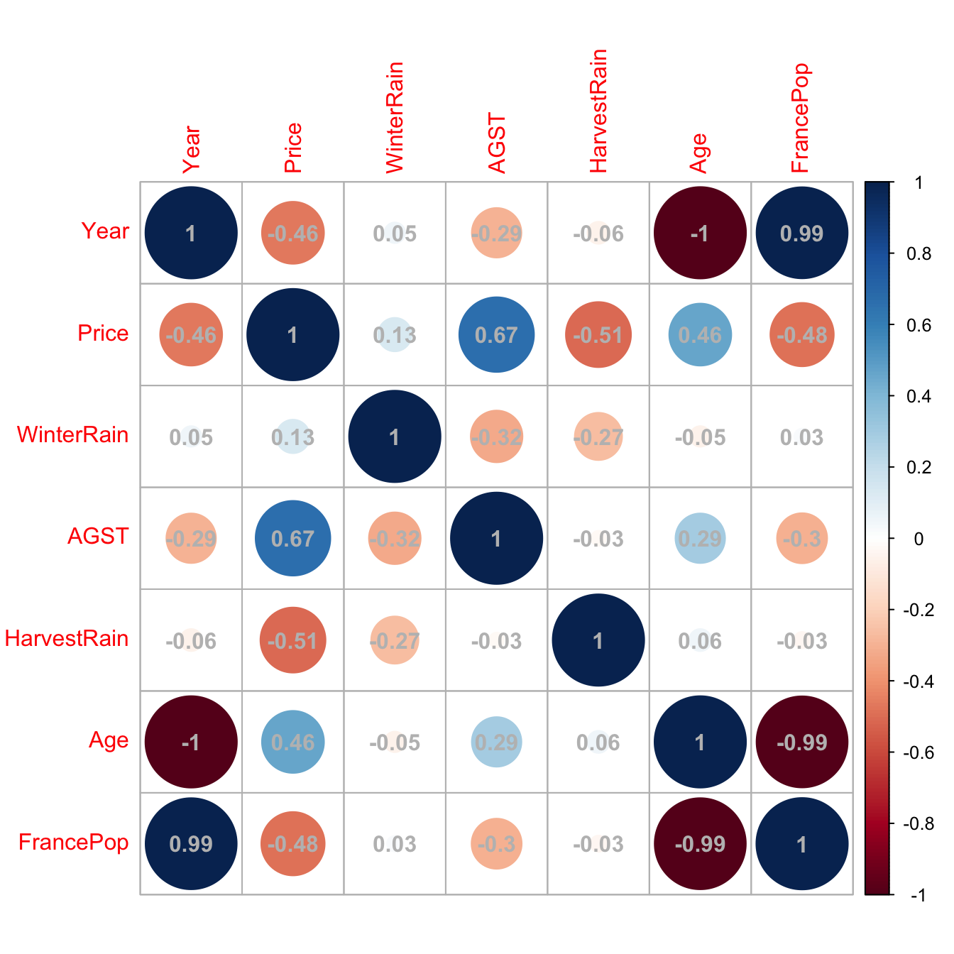

Figure 3.28: Graphical visualization of the correlation matrix.

Here we can see what we already knew from Section 2.1: Age and Year are perfectly linearly related and Age and FrancePop are highly linearly related. Then one approach will be to directly remove one of the highly-correlated predictors.

However, it is not enough to inspect pairwise correlations in order to get rid of multicollinearity. Indeed, it is possible to build counterexamples that show non-suspicious pairwise correlations but problematic complex linear relations that remain hidden. For the sake of illustration, here is one:

# Create predictors with multicollinearity: x4 depends on the rest
set.seed(45678)
x1 <- rnorm(100)
x2 <- 0.5 * x1 + rnorm(100)
x3 <- 0.5 * x2 + rnorm(100)
x4 <- -x1 + x2 + rnorm(100, sd = 0.25)

# Response
y <- 1 + 0.5 * x1 + 2 * x2 - 3 * x3 - x4 + rnorm(100)
data <- data.frame(x1 = x1, x2 = x2, x3 = x3, x4 = x4, y = y)

# Correlations -- none seems suspicious
corrplot::corrplot(cor(data), addCoef.col = "grey")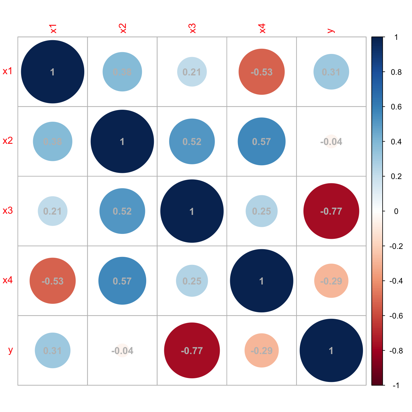

Figure 3.29: Unsuspicious correlation matrix with hidden multicollinearity.

A better approach to detect multicollinearity is to compute the Variance Inflation Factor (VIF) of each fitted coefficient \(\hat\beta_j.\) This is a measure of how linearly dependent is \(X_j\) on the rest of the predictors⁷⁹ and it is defined as

\[\begin{align*} \text{VIF}(\hat\beta_j)=\frac{1}{1-R^2_{X_j \mid X_{-j}}}, \end{align*}\]

where \(R^2_{X_j \mid X_{-j}}\) represents the \(R^2\) from the regression of \(X_j\) onto the remaining predictors \(X_1,\ldots,X_{j-1},X_{j+1}\ldots,X_p.\) Clearly, \(\text{VIF}(\hat\beta_j)\geq 1.\) The next simple rule of thumb gives direct insight into which predictors are multicollinear:

• VIF close to \(1\): absence of multicollinearity.
• VIF larger than \(5\) or \(10\): problematic amount of multicollinearity. Advised to remove the predictor with largest VIF.

VIF is computed with the car::vif function, which takes as an argument a linear model. Let’s see how it works in the previous example with hidden multicollinearity.

# Abnormal variance inflation factors: largest for x4, we remove it
modMultiCo <- lm(y ~ x1 + x2 + x3 + x4)
car::vif(modMultiCo)
##        x1        x2        x3        x4 
## 26.361444 29.726498  1.416156 33.293983

# Without x4
modClean <- lm(y ~ x1 + x2 + x3)

# Comparison
car::compareCoefs(modMultiCo, modClean)
## Calls:
## 1: lm(formula = y ~ x1 + x2 + x3 + x4)
## 2: lm(formula = y ~ x1 + x2 + x3)
## 
##             Model 1 Model 2
## (Intercept)   1.062   1.058
## SE            0.103   0.103
##                            
## x1            0.922   1.450
## SE            0.551   0.116
##                            
## x2            1.640   1.119
## SE            0.546   0.124
##                            
## x3           -3.165  -3.145
## SE            0.109   0.107
##                            
## x4           -0.529        
## SE            0.541        
## 
confint(modMultiCo)
##                  2.5 %     97.5 %
## (Intercept)  0.8568419  1.2674705
## x1          -0.1719777  2.0167093
## x2           0.5556394  2.7240952
## x3          -3.3806727 -2.9496676
## x4          -1.6030032  0.5446479
confint(modClean)
##                  2.5 %    97.5 %
## (Intercept)  0.8526681  1.262753
## x1           1.2188737  1.680188
## x2           0.8739264  1.364981
## x3          -3.3564513 -2.933473

# Summaries
summary(modMultiCo)
## 
## Call:
## lm(formula = y ~ x1 + x2 + x3 + x4)
## 
## Residuals:
##     Min      1Q  Median      3Q     Max 
## -1.9762 -0.6663  0.1195  0.6217  2.5568 
## 
## Coefficients:
##             Estimate Std. Error t value Pr(>|t|)    
## (Intercept)   1.0622     0.1034  10.270  < 2e-16 ***
## x1            0.9224     0.5512   1.673  0.09756 .  
## x2            1.6399     0.5461   3.003  0.00342 ** 
## x3           -3.1652     0.1086 -29.158  < 2e-16 ***
## x4           -0.5292     0.5409  -0.978  0.33040    
## ---
## Signif. codes:  0 '***' 0.001 '**' 0.01 '*' 0.05 '.' 0.1 ' ' 1
## 
## Residual standard error: 1.028 on 95 degrees of freedom
## Multiple R-squared:  0.9144, Adjusted R-squared:  0.9108 
## F-statistic: 253.7 on 4 and 95 DF,  p-value: < 2.2e-16
summary(modClean)
## 
## Call:
## lm(formula = y ~ x1 + x2 + x3)
## 
## Residuals:
##      Min       1Q   Median       3Q      Max 
## -1.91297 -0.66622  0.07889  0.65819  2.62737 
## 
## Coefficients:
##             Estimate Std. Error t value Pr(>|t|)    
## (Intercept)   1.0577     0.1033   10.24  < 2e-16 ***
## x1            1.4495     0.1162   12.47  < 2e-16 ***
## x2            1.1195     0.1237    9.05 1.63e-14 ***
## x3           -3.1450     0.1065  -29.52  < 2e-16 ***
## ---
## Signif. codes:  0 '***' 0.001 '**' 0.01 '*' 0.05 '.' 0.1 ' ' 1
## 
## Residual standard error: 1.028 on 96 degrees of freedom
## Multiple R-squared:  0.9135, Adjusted R-squared:  0.9108 
## F-statistic:   338 on 3 and 96 DF,  p-value: < 2.2e-16

# Variance inflation factors are normal
car::vif(modClean)
##       x1       x2       x3 
## 1.171942 1.525501 1.364878

Note that multicollinearity is another instance of the model correctness vs. usefulness. A model with multicollinearity might be perfectly valid in the sense of respecting the assumptions of the model. As we saw in Section 2.3, it does not matter whether the predictors are related or not, at least for the verification of the assumptions. But the model will be useless if the multicollinearity is high, since it can inflate the variability of the estimation without any kind of bound. In the extreme case in which the multicollinearity is perfect, then the model will not be identifiable, despite being correct.

The next simulation study illustrates how the non-identifiability of \(\boldsymbol\beta\) worsens with increasing multicollinearity, and therefore so does the error on estimating \(\boldsymbol\beta.\) We consider the linear model \[\begin{align*} Y=X_1+X_2+X_3+\varepsilon,\quad \varepsilon\sim\mathcal{N}(0, 1), \end{align*}\] where \[\begin{align*} X_1,X_2\sim\mathcal{N}(0,1),\quad X_3=b(X_1+X_2)+\delta,\quad \delta\sim \mathcal{N}(0, 0.25) \end{align*}\] and \(b\geq0\) controls the degree of multicollinearity of \(X_3\) with \(X_1\) and \(X_2\) (if \(b=0,\) \(X_3\) is uncorrelated with \(X_1\) and \(X_2\)). We aim to study how \(\mathbb{E}[\|\hat{\boldsymbol{\beta}}-\boldsymbol{\beta}\|]\) behaves when \(n\) grows, for different values of \(b.\) To do so, we consider \(n=2^\ell,\) \(\ell=3,\ldots,12,\) \(b=0,0.5,1,5,10,\) and approximate the expected error by Monte Carlo using \(M=500\) replicates. The results of the simulation study are shown in Figure 3.30, which illustrates that multicollinearity notably decreases the accuracy of \(\hat{\boldsymbol{\beta}},\) at all sample sizes \(n.\)

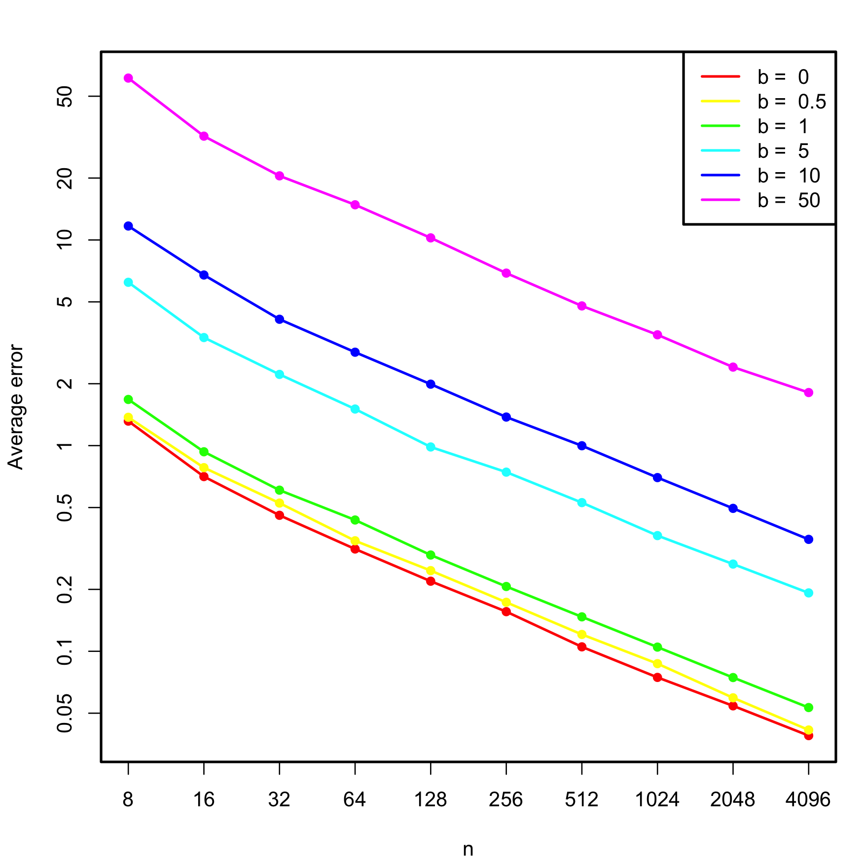
Figure 3.30: Estimated average error \(\mathbb{E}\lbrack\|\hat{\boldsymbol{\beta}}-\boldsymbol{\beta}\|\rbrack,\) for varying \(n\) and degrees of multicollinearity, indexed by \(b.\) The horizontal and vertical axes are in logarithmic scales.

Exercise 3.10 Replicate Figure 3.30 by implementing the simulation study behind it.

3.5.6 Outliers and high-leverage points

Outliers and high-leverage points are particular observations that have an important impact in the final linear model, either on the estimates or on the properties of the model. They are defined as follows:

• Outliers are the observations with a response \(Y_i\) far away from the regression plane. They typically do not affect the estimate of the plane, unless one of the predictors is also extreme (see next point). But they inflate \(\hat\sigma\) and, as a consequence, they draw down the \(R^2\) of the model and expand the CIs.
• High-leverage points are observations with an extreme predictor \(X_{ij}\) located far away from the rest of points. These observations are highly influential and may drive the linear model fit. The reason is the squared distance in the RSS: an individual extreme point may represent a large portion of the RSS.

Both outliers and high-leverage points can be identified with the residuals vs. leverage plot:

plot(mod, 5)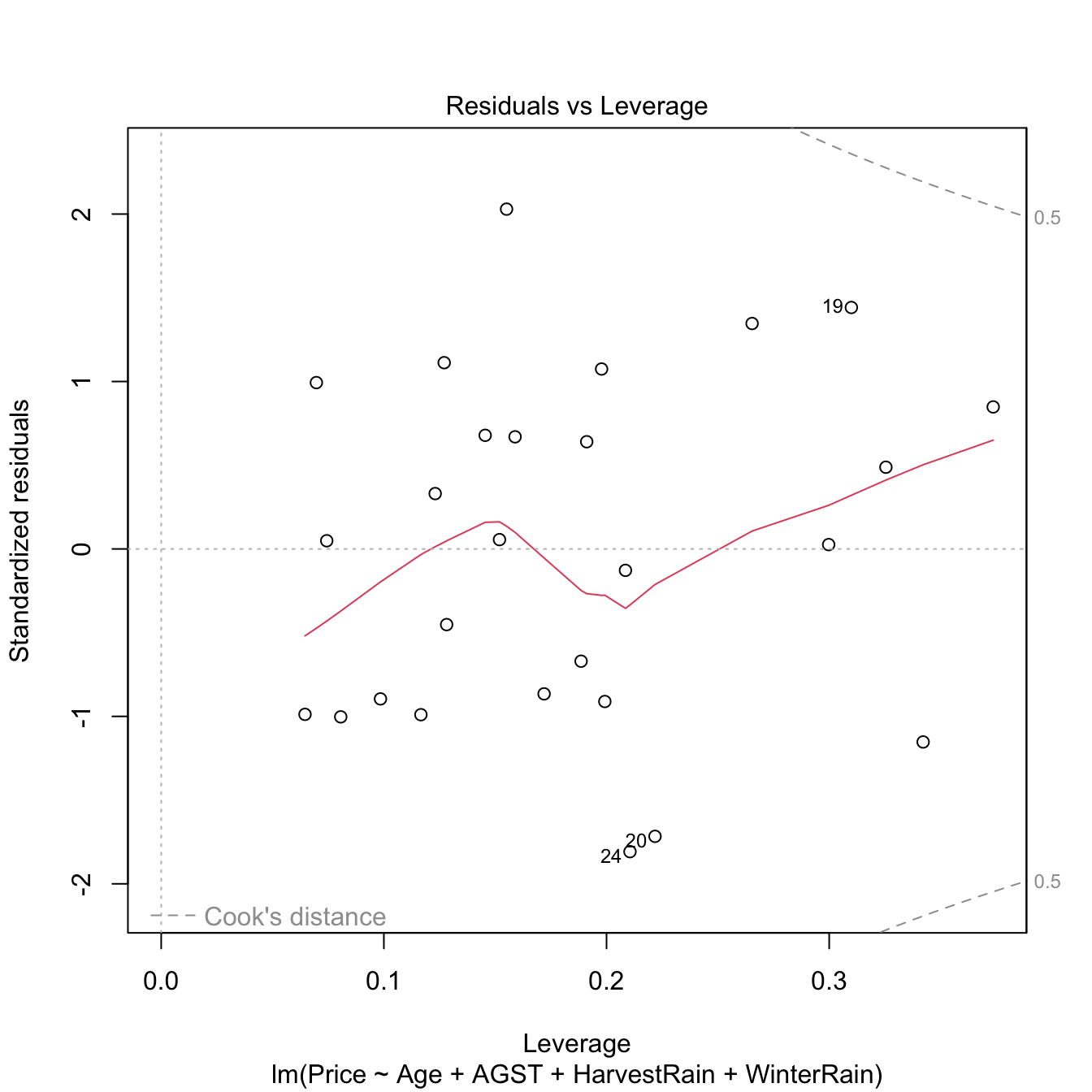

Figure 3.31: Residuals vs. leverage plot for the Price ~ Age + AGST + HarvestRain + WinterRain model for the wine dataset.

The rules of thumb for declaring outliers and high-leverage points are:

• If the standardized residual of an observation is larger than \(3\) in absolute value, then it may be an outlier.
• If the leverage statistic \(h_i\) is greatly exceeding \((p+1)/n\;\)⁸⁰ (see below), then the \(i\)-th observation may be suspected of having a high leverage.

Let’s see an artificial example.

# Create data
set.seed(12345)
x <- rnorm(100)
e <- rnorm(100, sd = 0.5)
y <- 1 + 2 * x + e

# Leverage expected value
2 / 101 # (p + 1) / n
## [1] 0.01980198

# Base model
m0 <- lm(y ~ x)
plot(x, y)
abline(coef = m0$coefficients, col = 2)

plot(m0, 5)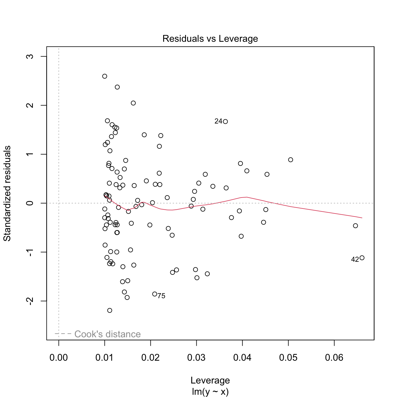

summary(m0)
## 
## Call:
## lm(formula = y ~ x)
## 
## Residuals:
##      Min       1Q   Median       3Q      Max 
## -1.10174 -0.30139 -0.00557  0.30949  1.30485 
## 
## Coefficients:
##             Estimate Std. Error t value Pr(>|t|)    
## (Intercept)  1.01103    0.05176   19.53   <2e-16 ***
## x            2.04727    0.04557   44.93   <2e-16 ***
## ---
## Signif. codes:  0 '***' 0.001 '**' 0.01 '*' 0.05 '.' 0.1 ' ' 1
## 
## Residual standard error: 0.5054 on 98 degrees of freedom
## Multiple R-squared:  0.9537, Adjusted R-squared:  0.9532 
## F-statistic:  2018 on 1 and 98 DF,  p-value: < 2.2e-16

# Make an outlier
x[101] <- 0; y[101] <- 30
m1 <- lm(y ~ x)
plot(x, y)
abline(coef = m1$coefficients, col = 2)

plot(m1, 5)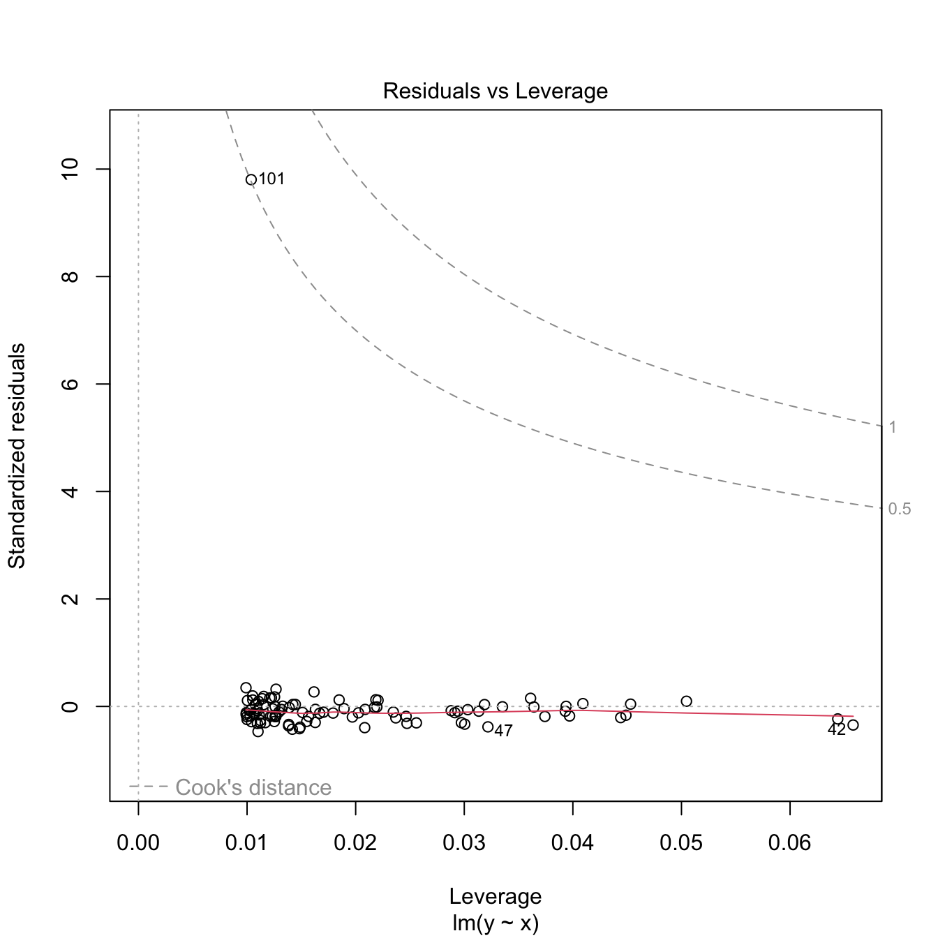

summary(m1)
## 
## Call:
## lm(formula = y ~ x)
## 
## Residuals:
##     Min      1Q  Median      3Q     Max 
## -1.3676 -0.5730 -0.2955  0.0941 28.6881 
## 
## Coefficients:
##             Estimate Std. Error t value Pr(>|t|)    
## (Intercept)   1.3119     0.2997   4.377 2.98e-05 ***
## x             1.9901     0.2652   7.505 2.71e-11 ***
## ---
## Signif. codes:  0 '***' 0.001 '**' 0.01 '*' 0.05 '.' 0.1 ' ' 1
## 
## Residual standard error: 2.942 on 99 degrees of freedom
## Multiple R-squared:  0.3627, Adjusted R-squared:  0.3562 
## F-statistic: 56.33 on 1 and 99 DF,  p-value: 2.708e-11

# Make a high-leverage point
x[101] <- 10; y[101] <- 5
m2 <- lm(y ~ x)
plot(x, y)
abline(coef = m2$coefficients, col = 2)

plot(m2, 5)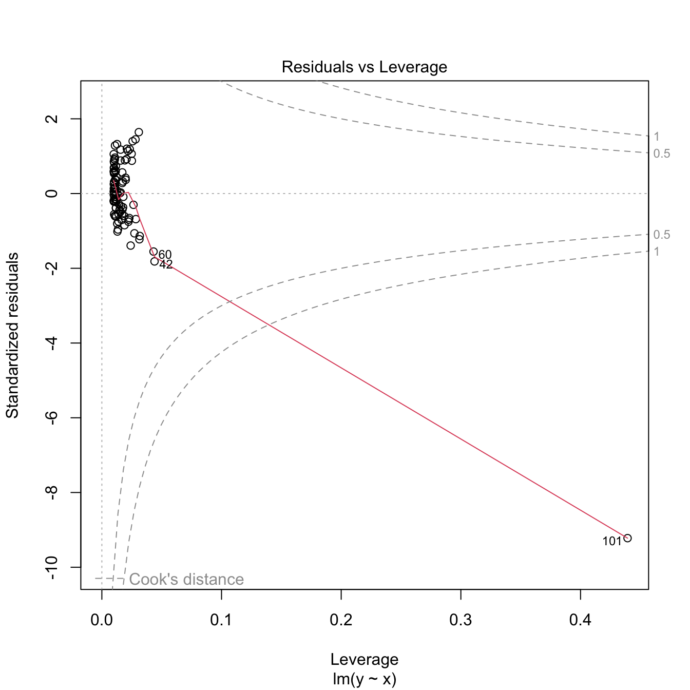

summary(m2)
## 
## Call:
## lm(formula = y ~ x)
## 
## Residuals:
##     Min      1Q  Median      3Q     Max 
## -9.2423 -0.6126  0.0373  0.7864  2.1652 
## 
## Coefficients:
##             Estimate Std. Error t value Pr(>|t|)    
## (Intercept)  1.09830    0.13676   8.031 2.06e-12 ***
## x            1.31440    0.09082  14.473  < 2e-16 ***
## ---
## Signif. codes:  0 '***' 0.001 '**' 0.01 '*' 0.05 '.' 0.1 ' ' 1
## 
## Residual standard error: 1.339 on 99 degrees of freedom
## Multiple R-squared:  0.6791, Adjusted R-squared:  0.6758 
## F-statistic: 209.5 on 1 and 99 DF,  p-value: < 2.2e-16

The leverage statistic associated to the \(i\)-th datum corresponds to the \(i\)-th diagonal entry of the hat matrix \(\mathbf{H}\):

\[\begin{align*} h_{i}:=\mathbf{H}_{ii}=(\mathbf{X}(\mathbf{X}^\top\mathbf{X})^{-1}\mathbf{X}^\top)_{ii}. \end{align*}\]

It can be seen that \(\frac{1}{n}\leq h_i\leq 1\) and that the mean \(\bar{h}=\frac{1}{n}\sum_{i=1}^nh_i=\frac{p+1}{n}.\) This can be clearly seen in the case of simple linear regression, where the leverage statistic has the explicit form

\[\begin{align*} h_{i}=\frac{1}{n}+\frac{(X_i-\bar{X})^2}{\sum_{j=1}^n(X_j-\bar{X})^2}. \end{align*}\]

Interestingly, this expression shows that the leverage statistic is directly dependent on the distance to the center of the predictor. A precise threshold for determining when \(h_i\) is greatly exceeding its expected value \(\bar{h}\) can be given if the predictors are assumed to be jointly normal. In this case, \(nh_i-1\sim\chi^2_p\) (Peña 2002) and hence the \(i\)-th point is declared as a potential high-leverage point if \(h_i>\frac{\chi^2_{p;\alpha}+1}{n},\) where \(\chi^2_{p;\alpha}\) is the \(\alpha\)-upper quantile of the \(\chi^2_p\) distribution (\(\alpha\) can be taken as \(0.05\) or \(0.01\)).

The functions influence, hat, and rstandard allow performing a finer inspection of the leverage statistics.

# Access leverage statistics
head(influence(model = m2, do.coef = FALSE)$hat)
##          1          2          3          4          5          6 
## 0.01017449 0.01052333 0.01083766 0.01281244 0.01022209 0.03137304

# Another option
h <- hat(x = x)

# 1% most influential points
n <- length(x)
p <- 1
hist(h, breaks = 20)
abline(v = (qchisq(0.99, df = p) + 1) / n, col = 2)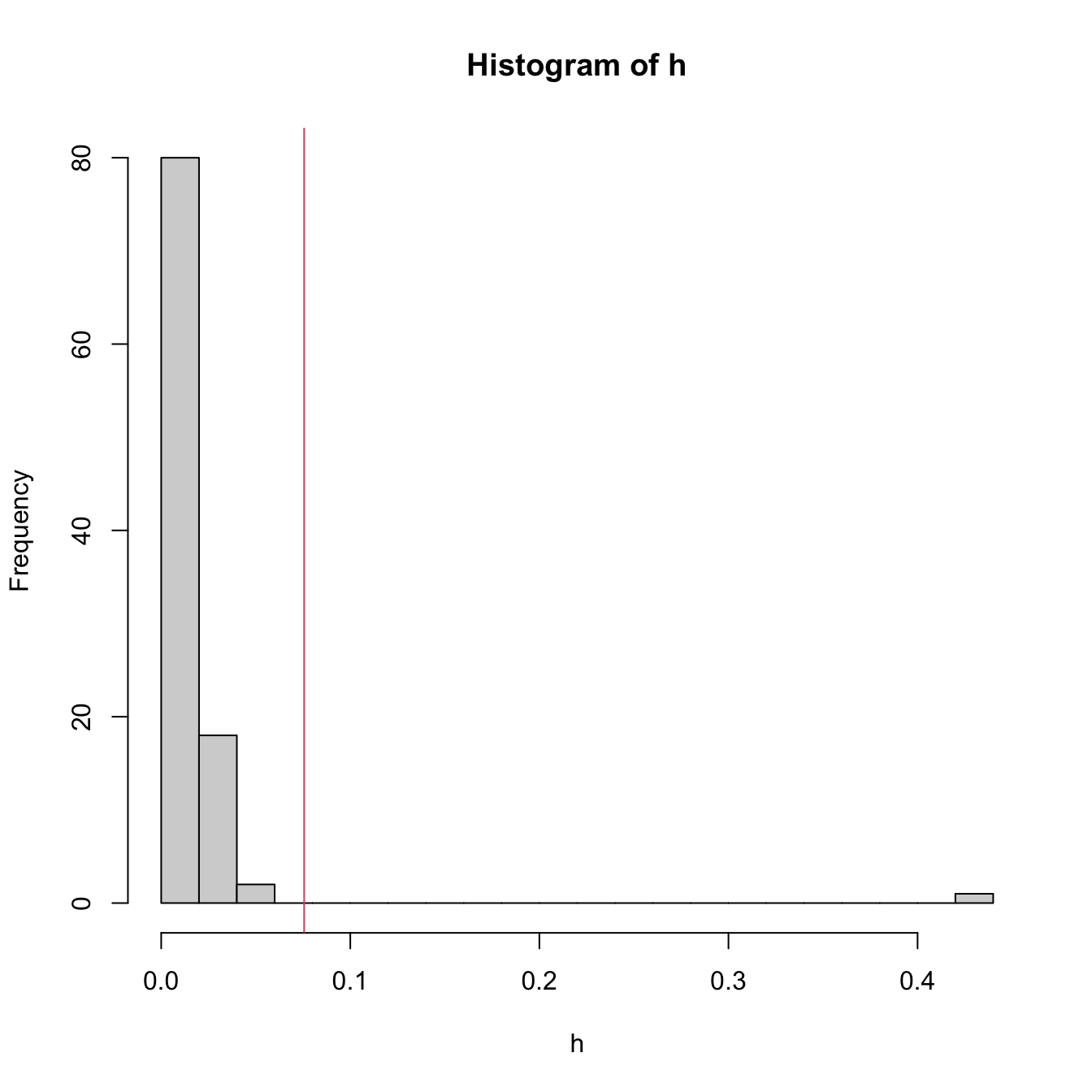

# Standardized residuals
rs <- rstandard(m2)
plot(m2, 2) # QQ-plot
points(qnorm(ppoints(n = n)), sort(rs), col = 2, pch = '+') # Manually computed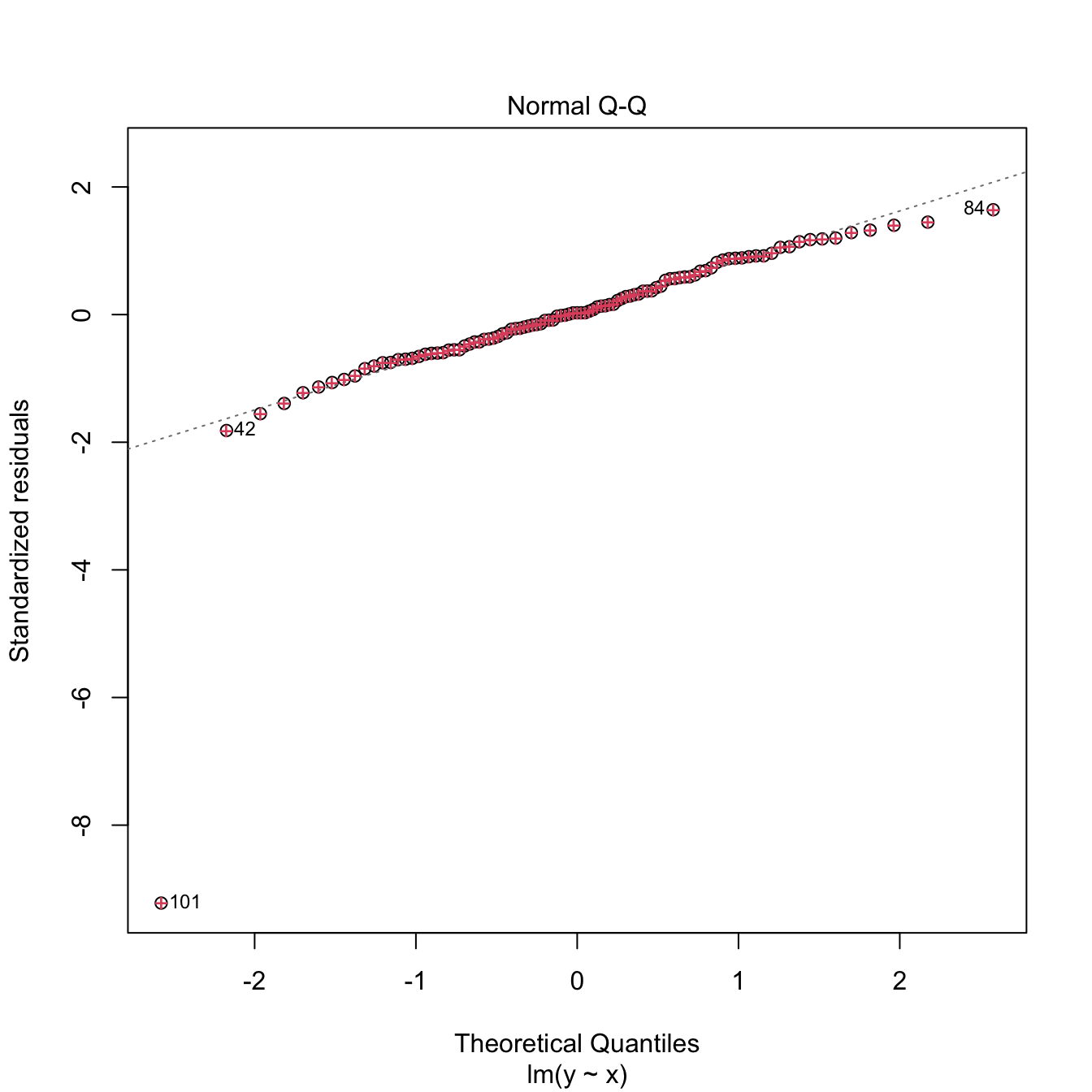

3.5.7 Case study application

Moore’s law (Moore 1965) is an empirical law that states that the power of a computer doubles approximately every two years. Translated into a mathematical formula, Moore’s law is

\[\begin{align*} \text{transistors}\approx 2^{\text{years}/2}. \end{align*}\]

Applying logarithms to both sides gives

\[\begin{align*} \log(\text{transistors})\approx \frac{\log(2)}{2}\text{years}. \end{align*}\]

We can write the above formula more generally as

\[\begin{align*} \log(\text{transistors})=\beta_0+\beta_1 \text{years}+\varepsilon, \end{align*}\]

where \(\varepsilon\) is a random error. This is a linear model!

Exercise 3.11 The dataset cpus.txt (source, retrieved in September 2016) contains the transistor counts for the CPUs appeared in the time range 1971–2015. For this data, do the following:

1. Import conveniently the data and name it as cpus.
2. Show a scatterplot of Transistor.count vs. Date.of.introduction with a linear regression.
3. Are the assumptions verified in Transistor.count ~ Date.of.introduction? Which ones are more “problematic”?
4. Create a new variable, named Log.Transistor.count, containing the logarithm of Transistor.count.
5. Show a scatterplot of Log.Transistor.count vs. Date.of.introduction with a linear regression.
6. Are the assumptions verified in Log.Transistor.count ~ Date.of.introduction? Which ones are more “problematic”?
7. Regress Log.Transistor.count ~ Date.of.introduction.
8. Summarize the fit. What are the estimates \(\hat\beta_0\) and \(\hat\beta_1\)? Is \(\hat\beta_1\) close to \(\frac{\log(2)}{2}\)?
9. Compute the CI for \(\beta_1\) at \(\alpha=0.05.\) Is \(\frac{\log(2)}{2}\) inside it? What happens at levels \(\alpha=0.10,0.01\)?
10. We want to forecast the average log-number of transistors for the CPUs to be released in 2024. Compute the adequate prediction and CI.
11. A new CPU design is expected for 2025. What is the range of log-number of transistors expected for it, at a \(95\%\) level of confidence?
12. Compute the ANOVA table for Log.Transistor.count ~ Date.of.introduction. Is \(\beta_1\) significant?

Exercise 3.12 The dataset gpus.txt (source, retrieved in September 2016) contains the transistor counts for the GPUs appeared in the period 1997–2016. Repeat the previous analysis for this dataset.

Exercise 3.13 Analyze the bias induced by transforming the response, fitting a linear model, and then untransforming. For that, consider the relation \[\begin{align} Y=\exp(\beta_0+\beta_1X+\varepsilon),\tag{3.8} \end{align}\] where \(X\sim\mathcal{N}(0,0.5)\) and \(\varepsilon\sim\mathcal{N}(0,1)\). Set \(\beta_0=-1\) and \(\beta_1=1.\) Then, follow these steps:

1. Compute the exact conditional distribution \(Y \mid X=x.\) Hint: use the lognormal distribution.
2. Based on Step 1, compute the true regression function \(m(x)=\mathbb{E}[Y \mid X=x]\) exactly and plot it.
3. Simulate a sample \(\{(X_i,Y_i)\}_{i=1}^n\) from (3.8), with \(n=200.\)
4. Define \(W:=\log(Y)\) and fit the linear model \(W=\beta_0+\) \(\beta_1X+\varepsilon\) from the previous sample. Are \((\beta_0,\beta_1)\) properly estimated?
5. Estimate \(\mathbb{E}[W \mid X=0]\) and \(\mathbb{E}[W \mid X=1]\) by \(\hat w_0=\hat\beta_0\) and \(\hat w_1=\hat\beta_0+\hat\beta_1,\) respectively.
6. Compute \(\hat y_0=\exp(\hat w_0)\) and \(\hat y_1=\exp(\hat w_1),\) the predictions with the transformed model of \(\mathbb{E}[Y \mid X=0]\) and \(\mathbb{E}[Y \mid X=1].\) Compare the estimates with \(m(0)\) and \(m(1).\)
7. Plot the fitted curve \(\hat y = \exp(\hat\beta_0+\hat\beta_1x)\) and compare with \(m\) in Step 2.
8. If \(n\) is increased in Step 3, does the estimation in Step 6 improve? Summarize your takeaways from the exercise.

3.6 Dimension reduction techniques

As we have seen in Section 3.2, the selection of the best linear model from a set of \(p\) predictors is a challenging task that increases with the dimension of the problem, that is, with \(p.\) In addition to the growth of the set of possible models as \(p\) grows, the model space becomes more complicated to explore due to the potential multicollinearity among the predictors. We will see in this section two methods to deal with these two problems simultaneously.

3.6.1 Review on principal component analysis

Principal Component Analysis (PCA) is a multivariate technique designed to summarize the most important features and relations of \(p\) numerical random variables \(X_1,\ldots,X_p.\) PCA computes a new set of variables, the principal components \(\Gamma_1,\ldots, \Gamma_p,\) that contain the same information as \(X_1,\ldots,X_p\) but expressed in a more convenient way. The goal of PCA is to retain only a limited number \(\ell,\) \(1\leq \ell\leq p,\) of principal components that explain most of the information, therefore performing dimension reduction.

If \(X_1,\ldots,X_p\) are centered,⁸¹ then the principal components are orthonormal linear combinations of \(X_1,\ldots,X_p\):

\[\begin{align} \Gamma_j:=a_{1j}X_1+a_{2j}X_2+\cdots+a_{pj}X_p=\mathbf{a}_j^\top\mathbf{X},\quad j=1,\ldots,p,\tag{3.9} \end{align}\]

where \(\mathbf{a}_j:=(a_{1j},\ldots,a_{pj})^\top,\) \(\mathbf{X}:=(X_1,\ldots,X_p)^\top,\) and the orthonormality condition is

\[\begin{align*} \mathbf{a}_i^\top\mathbf{a}_j=\begin{cases}1,&\text{if } i=j,\\0,&\text{if } i\neq j.\end{cases} \end{align*}\]

Remarkably, PCA computes the principal components in an ordered way: \(\Gamma_1\) is the principal component that explains the most of the information (quantified as the variance) of \(X_1,\ldots,X_p,\) and then the explained information decreases monotonically down to \(\Gamma_p,\) the principal component that explains the least information. Precisely:

\[\begin{align} \mathbb{V}\mathrm{ar}[\Gamma_1]\geq \mathbb{V}\mathrm{ar}[\Gamma_2]\geq\ldots\geq\mathbb{V}\mathrm{ar}[\Gamma_p].\tag{3.10} \end{align}\]

Mathematically, PCA computes the spectral decomposition⁸² of the covariance matrix \(\boldsymbol\Sigma:=\mathbb{V}\mathrm{ar}[\mathbf{X}]\):

\[\begin{align*} \boldsymbol\Sigma=\mathbf{A}\boldsymbol\Lambda\mathbf{A}^\top, \end{align*}\]

where \(\boldsymbol\Lambda=\mathrm{diag}(\lambda_1,\ldots,\lambda_p)\) contains the eigenvalues of \(\boldsymbol\Sigma\) and \(\mathbf{A}\) is the orthogonal matrix⁸³ whose columns are the unit-norm eigenvectors of \(\boldsymbol\Sigma.\) The matrix \(\mathbf{A}\) gives, thus, the coefficients of the orthonormal linear combinations:

\[\begin{align*} \mathbf{A}=\begin{pmatrix} \mathbf{a}_1 & \mathbf{a}_2 & \cdots & \mathbf{a}_p \end{pmatrix}=\begin{pmatrix} a_{11} & a_{12} & \cdots & a_{1p} \\ a_{21} & a_{22} & \cdots & a_{2p} \\ \vdots & \vdots & \ddots & \vdots \\ a_{p1} & a_{p2} & \cdots & a_{pp} \end{pmatrix}. \end{align*}\]

If the variables are not centered, the computation of the principal components is done by first subtracting \(\boldsymbol\mu=\mathbb{E}[\mathbf{X}]\) and then premultiplying with \(\mathbf{A}^\top\):

\[\begin{align} \boldsymbol{\Gamma}=\mathbf{A}^\top(\mathbf{X}-\boldsymbol{\mu}),\tag{3.11} \end{align}\]

where \(\boldsymbol{\Gamma}=(\Gamma_1,\ldots,\Gamma_p)^\top,\) \(\mathbf{X}=(X_1,\ldots,X_p)^\top,\) and \(\boldsymbol{\mu}=(\mu_1,\ldots,\mu_p)^\top.\) Note that, because of (1.3) and (3.11),

\[\begin{align} \mathbb{V}\mathrm{ar}[\boldsymbol{\Gamma}]=\mathbf{A}^\top\boldsymbol{\Sigma}\mathbf{A}=\mathbf{A}^\top\mathbf{A}\boldsymbol{\Lambda}\mathbf{A}^\top\mathbf{A}=\boldsymbol{\Lambda}. \end{align}\]

Therefore, \(\mathbb{V}\mathrm{ar}[\Gamma_j]=\lambda_j,\) \(j=1,\ldots,p,\) and as a consequence (3.10) indeed holds.

Also, from (3.11), it is evident that we can express the random vector \(\mathbf{X}\) in terms of \(\boldsymbol{\Gamma}\):

\[\begin{align} \mathbf{X}=\boldsymbol{\mu}+\mathbf{A}\boldsymbol{\Gamma},\tag{3.12} \end{align}\]

which admits an insightful interpretation: \(\boldsymbol{\Gamma}\) is an uncorrelated⁸⁴ vector that, once rotated by \(\mathbf{A}\) and translated to the location \(\boldsymbol{\mu},\) produces exactly \(\mathbf{X}.\) Therefore, \(\boldsymbol{\Gamma}\) contains the same information as \(\mathbf{X}\) but rearranged in a more convenient way, because the principal components are centered and uncorrelated between them:

\[\begin{align*} \mathbb{E}[\Gamma_i]=0\text{ and }\mathrm{Cov}[\Gamma_i,\Gamma_j]=\begin{cases}\lambda_i,&\text{if } i=j,\\0,&\text{if } i\neq j.\end{cases} \end{align*}\]

Due to the uncorrelation of \(\boldsymbol{\Gamma},\) we can measure the total variance of \(\boldsymbol{\Gamma}\) as \(\sum_{j=1}^p\mathbb{V}\mathrm{ar}[\Gamma_j]=\sum_{j=1}^p\lambda_j.\) Consequently, we can define the proportion of variance explained by the first \(\ell\) principal components, \(1\leq \ell\leq p,\) as

\[\begin{align*} \frac{\sum_{j=1}^\ell\lambda_j}{\sum_{j=1}^p\lambda_j}. \end{align*}\]

In the sample case⁸⁵ where a sample \(\mathbf{X}_1,\ldots,\mathbf{X}_n\) is given and \(\boldsymbol\mu\) and \(\boldsymbol\Sigma\) are unknown, \(\boldsymbol\mu\) is replaced by the sample mean \(\bar{\mathbf{X}}\) and \(\boldsymbol\Sigma\) by the sample variance-covariance matrix \(\mathbf{S}=\frac{1}{n}\sum_{i=1}^n(\mathbf{X}_i-\bar{\mathbf{X}})(\mathbf{X}_i-\bar{\mathbf{X}})^\top.\) Then, the spectral decomposition of \(\mathbf{S}\) is computed⁸⁶. This gives \(\hat{\mathbf{A}},\) the matrix of loadings, and produces the scores of the data:

\[\begin{align*} \hat{\boldsymbol{\Gamma}}_1:=\hat{\mathbf{A}}^\top(\mathbf{X}_1-\bar{\mathbf{X}}),\ldots,\hat{\boldsymbol{\Gamma}}_n:=\hat{\mathbf{A}}^\top(\mathbf{X}_n-\bar{\mathbf{X}}). \end{align*}\]

The scores are centered, uncorrelated, and have sample variances in each vector’s entry that are sorted in a decreasing way. The scores are the data coordinates with respect to the principal component basis.

The maximum number of principal components that can be determined from a sample \(\mathbf{X}_1,\ldots,\mathbf{X}_n\) is \(\min(n-1,p),\) assuming that the matrix formed by \(\left(\mathbf{X}_1 \cdots \mathbf{X}_n\right)\) is of full rank (i.e., if the rank is \(\min(n,p)\)). If \(n\geq p\) and the variables \(X_1,\ldots,X_p\) are such that only \(r\) of them are linearly independent, then the maximum is \(\min(n-1,r).\)

Let’s see an example of these concepts in La Liga 2015/2016 dataset. It contains the standings and team statistics for La Liga 2015/2016.

laliga <- readxl::read_excel("la-liga-2015-2016.xlsx", sheet = 1, col_names = TRUE)
laliga <- as.data.frame(laliga) # Avoid tibble since it drops row.names

A quick preprocessing gives:

rownames(laliga) <- laliga$Team # Set teams as case names to avoid factors
laliga$Team <- NULL
laliga <- laliga[, -c(2, 8)] # Do not add irrelevant information
summary(laliga)
##      Points           Wins           Draws           Loses        Goals.scored    Goals.conceded 
##  Min.   :32.00   Min.   : 8.00   Min.   : 4.00   Min.   : 4.00   Min.   : 34.00   Min.   :18.00  
##  1st Qu.:41.25   1st Qu.:10.00   1st Qu.: 8.00   1st Qu.:12.00   1st Qu.: 40.00   1st Qu.:42.50  
##  Median :44.50   Median :12.00   Median : 9.00   Median :15.50   Median : 45.50   Median :52.50  
##  Mean   :52.40   Mean   :14.40   Mean   : 9.20   Mean   :14.40   Mean   : 52.15   Mean   :52.15  
##  3rd Qu.:60.50   3rd Qu.:17.25   3rd Qu.:10.25   3rd Qu.:18.25   3rd Qu.: 51.25   3rd Qu.:63.25  
##  Max.   :91.00   Max.   :29.00   Max.   :18.00   Max.   :22.00   Max.   :112.00   Max.   :74.00  
##  Percentage.scored.goals Percentage.conceded.goals     Shots       Shots.on.goal   Penalties.scored  Assistances   
##  Min.   :0.890           Min.   :0.470             Min.   :346.0   Min.   :129.0   Min.   : 1.00    Min.   :23.00  
##  1st Qu.:1.050           1st Qu.:1.115             1st Qu.:413.8   1st Qu.:151.2   1st Qu.: 1.00    1st Qu.:28.50  
##  Median :1.195           Median :1.380             Median :438.0   Median :165.0   Median : 3.00    Median :32.50  
##  Mean   :1.371           Mean   :1.371             Mean   :452.4   Mean   :173.1   Mean   : 3.45    Mean   :37.85  
##  3rd Qu.:1.347           3rd Qu.:1.663             3rd Qu.:455.5   3rd Qu.:180.0   3rd Qu.: 4.50    3rd Qu.:36.75  
##  Max.   :2.950           Max.   :1.950             Max.   :712.0   Max.   :299.0   Max.   :11.00    Max.   :90.00  
##    Fouls.made    Matches.without.conceding  Yellow.cards     Red.cards       Offsides     
##  Min.   :385.0   Min.   : 4.0              Min.   : 66.0   Min.   :1.00   Min.   : 72.00  
##  1st Qu.:483.8   1st Qu.: 7.0              1st Qu.: 97.0   1st Qu.:4.00   1st Qu.: 83.25  
##  Median :530.5   Median :10.5              Median :108.5   Median :5.00   Median : 88.00  
##  Mean   :517.6   Mean   :10.7              Mean   :106.2   Mean   :5.05   Mean   : 92.60  
##  3rd Qu.:552.8   3rd Qu.:13.0              3rd Qu.:115.2   3rd Qu.:6.00   3rd Qu.:103.75  
##  Max.   :654.0   Max.   :24.0              Max.   :141.0   Max.   :9.00   Max.   :123.00

Let’s check that R’s function for PCA, princomp, returns the same principal components we outlined in the theory.

# PCA
pcaLaliga <- princomp(laliga, fix_sign = TRUE)
summary(pcaLaliga)
## Importance of components:
##                             Comp.1     Comp.2      Comp.3      Comp.4      Comp.5     Comp.6      Comp.7      Comp.8
## Standard deviation     104.7782561 48.5461449 22.13337511 12.66692413 8.234215354 7.83426116 6.068864168 4.137079559
## Proportion of Variance   0.7743008  0.1662175  0.03455116  0.01131644 0.004782025 0.00432876 0.002597659 0.001207133
## Cumulative Proportion    0.7743008  0.9405183  0.97506949  0.98638593 0.991167955 0.99549671 0.998094374 0.999301507
##                              Comp.9      Comp.10      Comp.11      Comp.12      Comp.13      Comp.14      Comp.15
## Standard deviation     2.0112480391 1.8580509157 1.126111e+00 9.568824e-01 4.716064e-01 1.707105e-03 8.365534e-04
## Proportion of Variance 0.0002852979 0.0002434908 8.943961e-05 6.457799e-05 1.568652e-05 2.055361e-10 4.935768e-11
## Cumulative Proportion  0.9995868048 0.9998302956 9.999197e-01 9.999843e-01 1.000000e+00 1.000000e+00 1.000000e+00
##                        Comp.16 Comp.17
## Standard deviation           0       0
## Proportion of Variance       0       0
## Cumulative Proportion        1       1
# The standard deviations are the square roots of the eigenvalues
# The cumulative proportion of variance explained accumulates the
# variance explained starting at the first component

# We use fix_sign = TRUE so that the signs of the loadings are
# determined by the first element of each loading, set to be
# nonnegative. Otherwise, the signs could change for different OS /
# R versions yielding to opposite interpretations of the PCs

# Plot of variances of each component (screeplot)
plot(pcaLaliga, type = "l")

# Useful for detecting an "elbow" in the graph whose location gives the
# "right" number of components to retain. Ideally, this elbow appears
# when the next variances are almost similar and notably smaller when
# compared with the previous

# Alternatively: plot of the cumulated percentage of variance
# barplot(cumsum(pcaLaliga$sdev^2) / sum(pcaLaliga$sdev^2))

# Computation of PCA from the spectral decomposition
n <- nrow(laliga)
eig <- eigen(cov(laliga) * (n - 1) / n) # By default, cov() computes the
# quasi-variance-covariance matrix that divides by n - 1, but PCA and princomp
# consider the sample variance-covariance matrix that divides by n
A <- eig$vectors

# Same eigenvalues
pcaLaliga$sdev^2 - eig$values
##        Comp.1        Comp.2        Comp.3        Comp.4        Comp.5        Comp.6        Comp.7        Comp.8 
## -5.456968e-12 -1.364242e-12  0.000000e+00 -4.263256e-13 -2.415845e-13 -1.278977e-13 -3.552714e-14 -4.263256e-14 
##        Comp.9       Comp.10       Comp.11       Comp.12       Comp.13       Comp.14       Comp.15       Comp.16 
## -2.025047e-13 -7.549517e-14 -1.088019e-14 -3.108624e-15 -1.626477e-14 -3.685726e-15  1.036604e-15 -2.025796e-13 
##       Comp.17 
##  1.435137e-12

# The eigenvectors (the a_j vectors) are the column vectors in $loadings
pcaLaliga$loadings
## 
## Loadings:
##                           Comp.1 Comp.2 Comp.3 Comp.4 Comp.5 Comp.6 Comp.7 Comp.8 Comp.9 Comp.10 Comp.11 Comp.12
## Points                     0.125         0.497  0.195  0.139  0.340         0.425         0.379   0.129   0.166 
## Wins                                     0.184                0.175         0.134 -0.198                  0.139 
## Draws                                                  0.101 -0.186                0.608  0.175   0.185  -0.251 
## Loses                                   -0.129        -0.114               -0.157 -0.410 -0.243  -0.166   0.112 
## Goals.scored               0.181         0.251 -0.186 -0.169  0.399  0.335 -0.603 -0.155  0.129   0.289  -0.230 
## Goals.conceded                          -0.471 -0.493 -0.277  0.257  0.280  0.441 -0.118  0.297                 
## Percentage.scored.goals                                                                                         
## Percentage.conceded.goals                                                                                       
## Shots                      0.718  0.442 -0.342  0.255  0.241         0.188                                      
## Shots.on.goal              0.386  0.213  0.182 -0.287 -0.532 -0.163 -0.599                                      
## Penalties.scored                                                           -0.350  0.258  0.378  -0.661   0.456 
## Assistances                0.148         0.198        -0.173  0.362  0.216  0.215  0.356 -0.685  -0.265         
## Fouls.made                -0.480  0.844  0.166               -0.110                                             
## Matches.without.conceding                0.151  0.129               -0.182  0.176 -0.369         -0.376  -0.411 
## Yellow.cards              -0.141  0.144 -0.363  0.113  0.225  0.637 -0.550 -0.126  0.156                        
## Red.cards                                                                         -0.123 -0.157   0.405   0.666 
## Offsides                          0.108  0.202 -0.696  0.647        -0.106                                      
##                           Comp.13 Comp.14 Comp.15 Comp.16 Comp.17
## Points                     0.138                   0.240   0.345 
## Wins                       0.147                          -0.904 
## Draws                     -0.304                   0.554  -0.215 
## Loses                      0.156                   0.794   0.130 
## Goals.scored              -0.153                                 
## Goals.conceded                                                   
## Percentage.scored.goals           -0.760  -0.650                 
## Percentage.conceded.goals          0.650  -0.760                 
## Shots                                                            
## Shots.on.goal                                                    
## Penalties.scored          -0.114                                 
## Assistances               -0.102                                 
## Fouls.made                                                       
## Matches.without.conceding -0.664                                 
## Yellow.cards                                                     
## Red.cards                 -0.587                                 
## Offsides                                                         
## 
##                Comp.1 Comp.2 Comp.3 Comp.4 Comp.5 Comp.6 Comp.7 Comp.8 Comp.9 Comp.10 Comp.11 Comp.12 Comp.13 Comp.14
## SS loadings     1.000  1.000  1.000  1.000  1.000  1.000  1.000  1.000  1.000   1.000   1.000   1.000   1.000   1.000
## Proportion Var  0.059  0.059  0.059  0.059  0.059  0.059  0.059  0.059  0.059   0.059   0.059   0.059   0.059   0.059
## Cumulative Var  0.059  0.118  0.176  0.235  0.294  0.353  0.412  0.471  0.529   0.588   0.647   0.706   0.765   0.824
##                Comp.15 Comp.16 Comp.17
## SS loadings      1.000   1.000   1.000
## Proportion Var   0.059   0.059   0.059
## Cumulative Var   0.882   0.941   1.000

# The scores is the representation of the data in the principal components -
# it has the same information as laliga
head(round(pcaLaliga$scores, 4))
##                   Comp.1   Comp.2  Comp.3   Comp.4  Comp.5  Comp.6  Comp.7  Comp.8  Comp.9 Comp.10 Comp.11 Comp.12
## Barcelona       242.2392 -21.5810 25.3801 -17.4375 -7.1797  9.0814 -5.5920 -7.3615 -0.3716  1.7161  0.0265 -1.0948
## Real Madrid     313.6026  63.2024 -8.7570   8.5558  0.7119  0.2221  6.7035  2.4456  1.8388 -2.9661 -0.1345  0.3410
## Atlético Madrid  45.9939  -0.6466 38.5410  31.3888  3.9163  3.2904  0.2432  5.0913 -3.0444  2.0975  0.6771 -0.3986
## Villarreal      -96.2201 -42.9329 50.0036 -11.2420 10.4733  2.4294 -3.0183  0.1958  1.2106 -1.7453  0.1351 -0.5735
## Athletic         14.5173 -16.1897 18.8840  -0.4122 -5.6491 -6.9330  8.0653  2.4783 -2.6921  0.8950  0.1542  1.4715
## Celta           -13.0748   6.7925  5.2271  -9.0945  6.1265 11.8795 -2.6148  6.9707  3.0826  0.3130  0.0860  1.9159
##                 Comp.13 Comp.14 Comp.15 Comp.16 Comp.17
## Barcelona        0.1516 -0.0010  -2e-04       0       0
## Real Madrid     -0.0332  0.0015   4e-04       0       0
## Atlético Madrid -0.1809  0.0005  -1e-04       0       0
## Villarreal      -0.5894 -0.0001  -2e-04       0       0
## Athletic         0.1109 -0.0031  -3e-04       0       0
## Celta            0.3722 -0.0018   3e-04       0       0

# Uncorrelated
corrplot::corrplot(cor(pcaLaliga$scores), addCoef.col = "gray")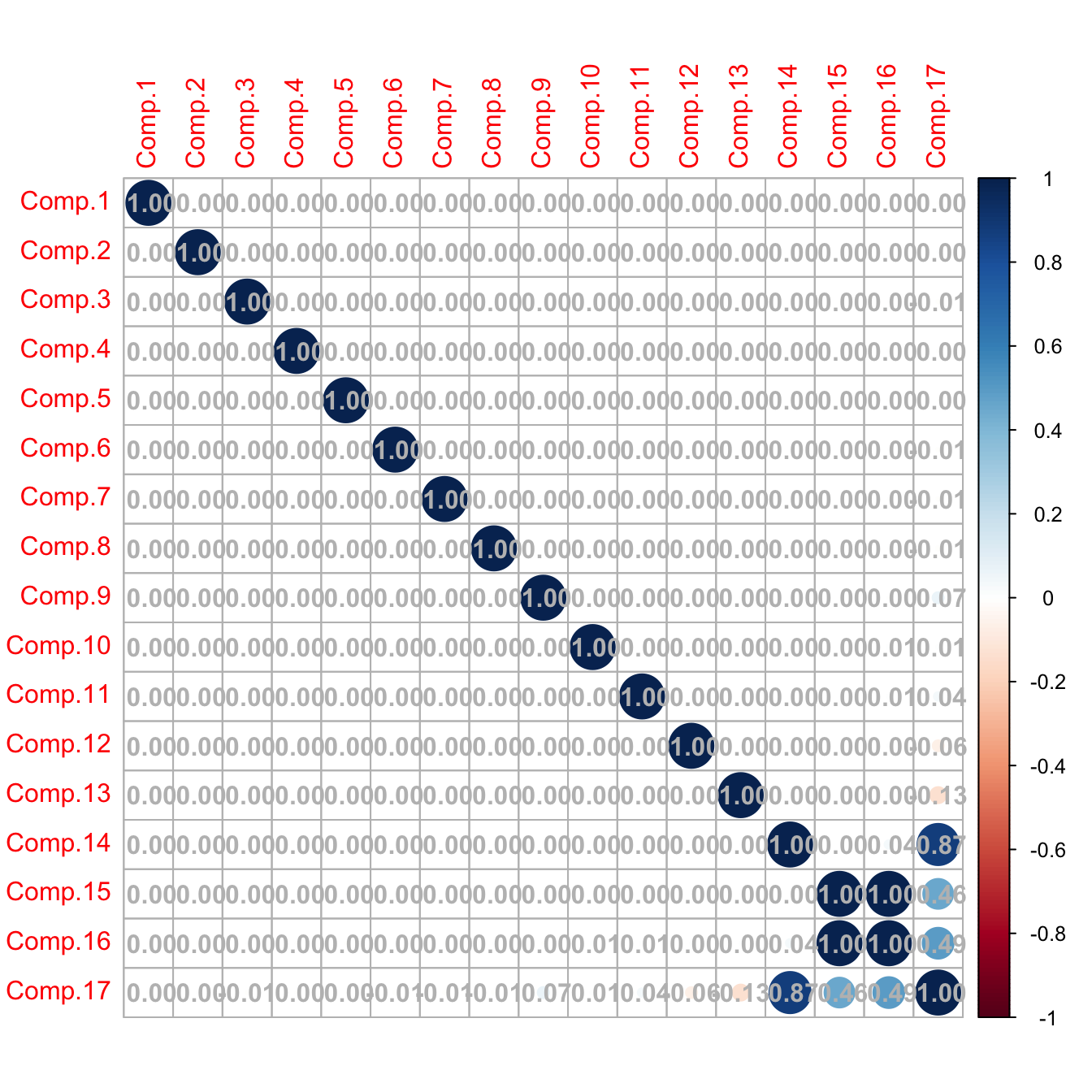

# Caution! What happened in the last columns? What happened is that the
# variance for the last principal components is close to zero (because there
# are linear dependencies on the variables; e.g., Points, Wins, Loses, Draws),
# so the computation of the correlation matrix becomes unstable for those
# variables (a 0/0 division takes place)

# Better to inspect the covariance matrix
corrplot::corrplot(cov(pcaLaliga$scores), addCoef.col = "gray", is.corr = FALSE)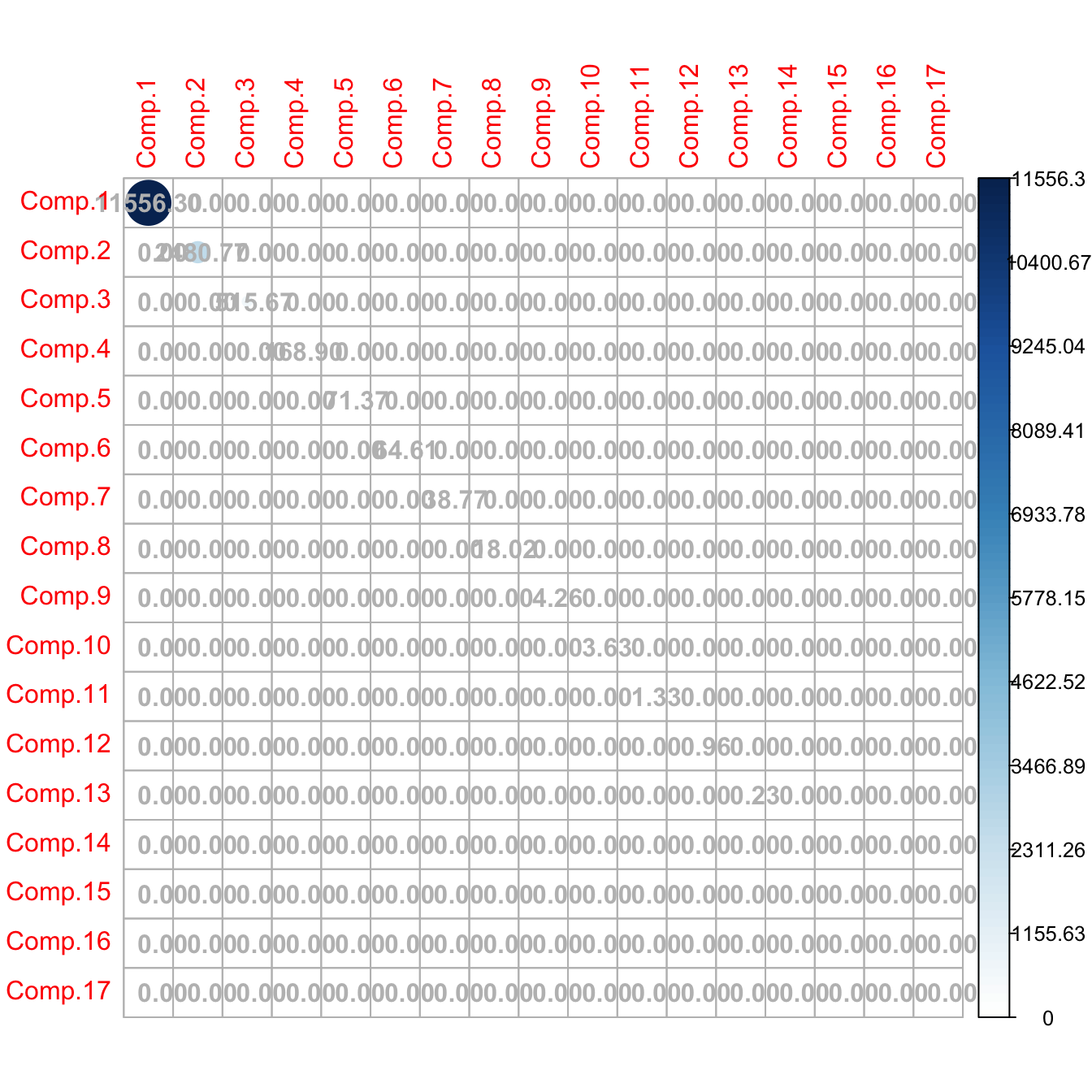

# The scores are A' * (X_i - mu). We center the data with scale()
# and then multiply each row by A'
scores <- scale(laliga, center = TRUE, scale = FALSE) %*% A

# Same as (but this is much slower)
# scores <- t(apply(scale(laliga, center = TRUE, scale = FALSE), 1,
#                   function(x) t(A) %*% x))

# Same scores (up to possible changes in signs)
max(abs(abs(pcaLaliga$scores) - abs(scores)))
## [1] 2.278507e-11

# Reconstruct the data from all the principal components
head(
  sweep(pcaLaliga$scores %*% t(pcaLaliga$loadings), 2, pcaLaliga$center, "+")
  )
##                 Points Wins Draws Loses Goals.scored Goals.conceded Percentage.scored.goals Percentage.conceded.goals
## Barcelona           91   29     4     5          112             29                    2.95                      0.76
## Real Madrid         90   28     6     4          110             34                    2.89                      0.89
## Atlético Madrid     88   28     4     6           63             18                    1.66                      0.47
## Villarreal          64   18    10    10           44             35                    1.16                      0.92
## Athletic            62   18     8    12           58             45                    1.53                      1.18
## Celta               60   17     9    12           51             59                    1.34                      1.55
##                 Shots Shots.on.goal Penalties.scored Assistances Fouls.made Matches.without.conceding Yellow.cards
## Barcelona         600           277               11          79        385                        18           66
## Real Madrid       712           299                6          90        420                        14           72
## Atlético Madrid   481           186                1          49        503                        24           91
## Villarreal        346           135                3          32        534                        17          100
## Athletic          450           178                3          42        502                        13           84
## Celta             442           170                4          43        528                        10          116
##                 Red.cards Offsides
## Barcelona               1      120
## Real Madrid             5      114
## Atlético Madrid         3       84
## Villarreal              4      106
## Athletic                5       92
## Celta                   6      103

An important issue when doing PCA is the scale of the variables, since the variance depends on the units in which the variable is measured.⁸⁷ Therefore, when variables with different ranges are mixed, the variability of one may dominate the other merely due to a scale artifact. To prevent this, we standardize the dataset prior to doing a PCA.

# Use cor = TRUE to standardize variables (all have unit variance)
# and avoid scale distortions
pcaLaligaStd <- princomp(x = laliga, cor = TRUE, fix_sign = TRUE)
summary(pcaLaligaStd)
## Importance of components:
##                           Comp.1    Comp.2     Comp.3     Comp.4     Comp.5     Comp.6     Comp.7      Comp.8
## Standard deviation     3.2918365 1.5511043 1.13992451 0.91454883 0.85765282 0.59351138 0.45780827 0.370649324
## Proportion of Variance 0.6374228 0.1415250 0.07643694 0.04919997 0.04326873 0.02072093 0.01232873 0.008081231
## Cumulative Proportion  0.6374228 0.7789478 0.85538472 0.90458469 0.94785342 0.96857434 0.98090308 0.988984306
##                             Comp.9     Comp.10     Comp.11      Comp.12     Comp.13      Comp.14      Comp.15
## Standard deviation     0.327182806 0.217470830 0.128381750 0.0976778705 0.083027923 2.582795e-03 1.226924e-03
## Proportion of Variance 0.006296976 0.002781974 0.000969522 0.0005612333 0.000405508 3.924019e-07 8.854961e-08
## Cumulative Proportion  0.995281282 0.998063256 0.999032778 0.9995940111 0.999999519 9.999999e-01 1.000000e+00
##                             Comp.16 Comp.17
## Standard deviation     9.256461e-09       0
## Proportion of Variance 5.040122e-18       0
## Cumulative Proportion  1.000000e+00       1

# The effects of the distortion can be clearly seen with the biplot
# Variability absorbed by Shots, Shots.on.goal, Fouls.made
biplot(pcaLaliga, cex = 0.75)

# The effects of the variables are more balanced
biplot(pcaLaligaStd, cex = 0.75)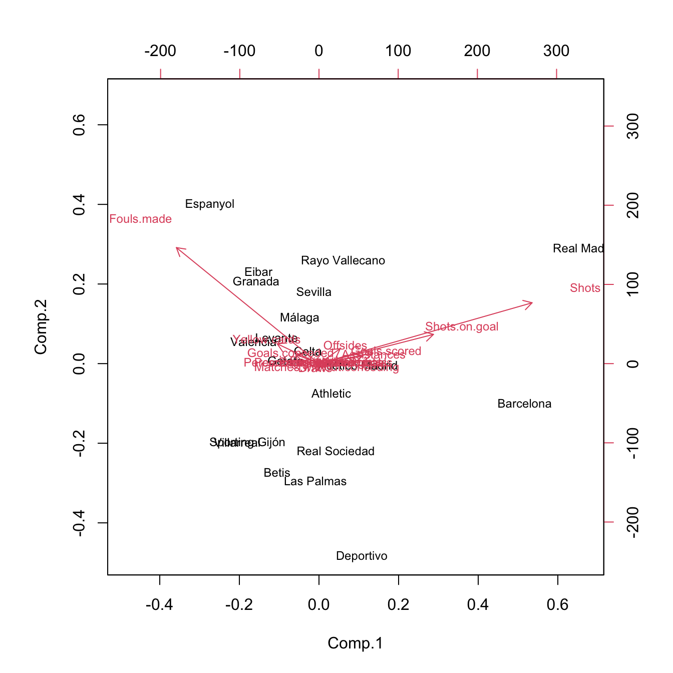

Figure 3.32: Biplots for laliga dataset, with unstandardized and standardized data, respectively.

The biplot⁸⁸ provides a powerful and succinct way of displaying the relevant information contained in the first two principal components. It shows:

1. The scores \(\{(\hat{\Gamma}_{i1},\hat{\Gamma}_{i2})\}_{i=1}^n\) by points (with optional text labels, depending if there are case names). These are the representations of the data in the first two principal components.
2. The loadings \(\{(\hat{a}_{j1},\hat{a}_{j2})\}_{j=1}^p\) by the arrows, centered at \((0,0).\) These are the representations of the variables in the first two principal components.

Let’s examine the population⁸⁹ arrow associated to the variable \(X_j.\) \(X_j\) is expressed in terms of \(\Gamma_1\) and \(\Gamma_2\) by the loadings \(a_{j1}\) and \(a_{j2}\;\)⁹⁰:

\[\begin{align*} X_j=a_{j1}\Gamma_{1} + a_{j2}\Gamma_{2} + \cdots + a_{jp}\Gamma_{p}\approx a_{j1}\Gamma_{1} + a_{j2}\Gamma_{2}. \end{align*}\]

The weights \(a_{j1}\) and \(a_{j2}\) have the same sign as \(\mathrm{Cor}(X_j,\Gamma_{1})\) and \(\mathrm{Cor}(X_j,\Gamma_{2}),\) respectively. The arrow associated to \(X_j\) is given by the segment joining \((0,0)\) and \((a_{j1},a_{j2}).\) Therefore:

• If the arrow points right (\(a_{j1}>0\)), there is positive correlation between \(X_j\) and \(\Gamma_1.\) Analogous if the arrow points left.
• If the arrow is approximately vertical (\(a_{j1}\approx0\)), there is uncorrelation between \(X_j\) and \(\Gamma_1.\)

Analogously:

• If the arrow points up (\(a_{j2}>0\)), there is positive correlation between \(X_j\) and \(\Gamma_2.\) Analogous if the arrow points down.
• If the arrow is approximately horizontal (\(a_{j2}\approx0\)), there is uncorrelation between \(X_j\) and \(\Gamma_2.\)

In addition, the magnitude of the arrow informs us about the strength of the correlation of \(X_j\) with \((\Gamma_{1}, \Gamma_{2}).\)

The biplot also informs about the direct relation between variables, at sight of their expressions in \(\Gamma_1\) and \(\Gamma_2.\) The angle of the arrows of variable \(X_j\) and \(X_k\) gives an approximation to the correlation between them, \(\mathrm{Cor}(X_j,X_k)\):

• If \(\text{angle}\approx 0^\circ,\) the two variables are highly positively correlated.
• If \(\text{angle}\approx 90^\circ,\) they are approximately uncorrelated.
• If \(\text{angle}\approx 180^\circ,\) the two variables are highly negatively correlated.

The insights obtained from the approximate correlations between variables are as precise as the percentage of variance explained by the first two principal components.

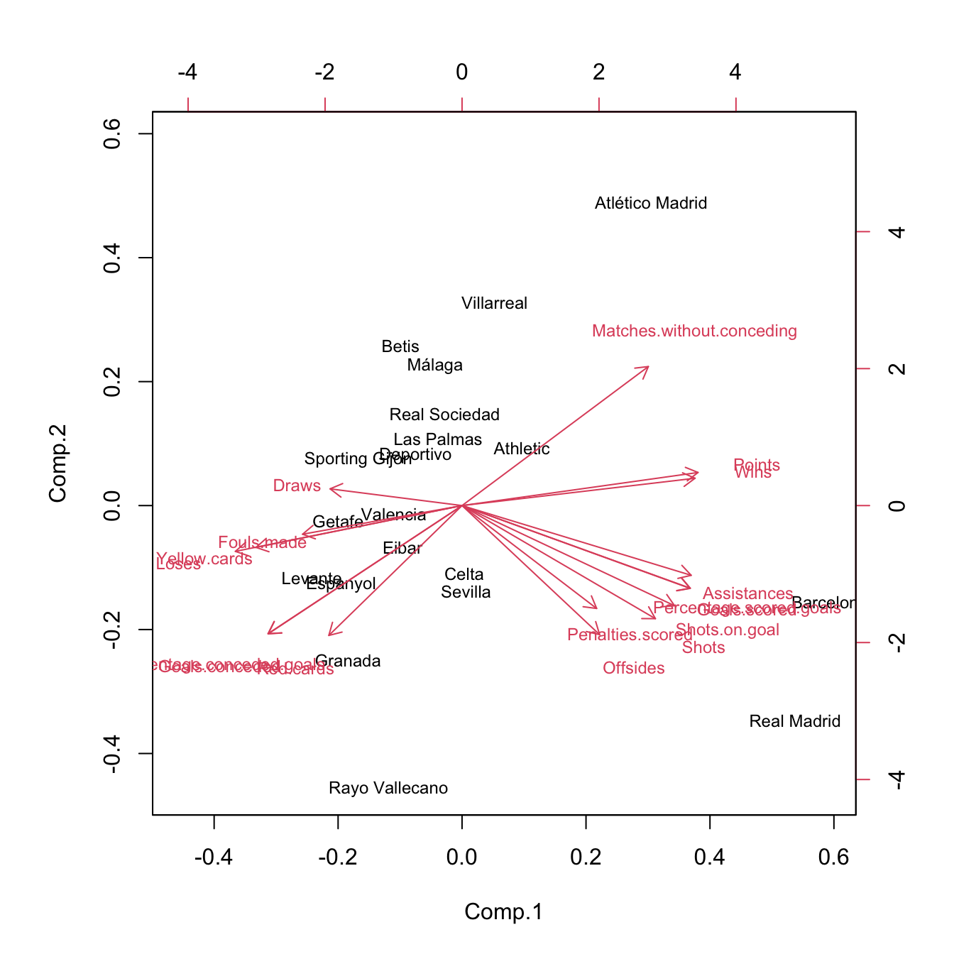
Figure 3.33: Biplot for laliga dataset. The interpretations of the first two principal components are driven by the signs of the variables inside them (directions of the arrows) and by the strength of their correlations with the variables (length of the arrows). The scores of the data serve also to cluster similar observations according to their proximity in the biplot.

Some interesting insights in La Liga 2015/2016 biplot, obtained from the previous remarks, are:⁹¹

• The first component can be regarded as the performance of a team during the season. It is positively correlated with Wins, Points, etc. and negatively correlated with Draws, Loses, Yellow.cards, etc. The best performing teams are not surprising: Barcelona, Real Madrid, and Atlético Madrid. On the other hand, among the worst-performing teams are Levante, Getafe, and Granada.
• The second component can be seen as the efficiency of a team (obtaining points with little participation in the game). Using this interpretation we can see that Atlético Madrid and Villareal were the most efficient teams and that Rayo Vallecano and Real Madrid were the most inefficient.
• Offsides is approximately uncorrelated with Red.cards and Matches.without.conceding.

A 3D representation of the biplot can be computed through:

pca3d::pca3d(pcaLaligaStd, show.labels = TRUE, biplot = TRUE)
## [1] 0.1747106 0.0678678 0.0799681
rgl::rglwidget()

Finally, the biplot function allows us to construct the biplot using two arbitrary principal components using the choices argument. Keep in mind than these pseudo-biplots will explain a lower proportion of variance than the default choices = 1:2:

biplot(pcaLaligaStd, choices = c(1, 3)) # 0.7138 proportion of variance
biplot(pcaLaligaStd, choices = c(2, 3)) # 0.2180 proportion of variance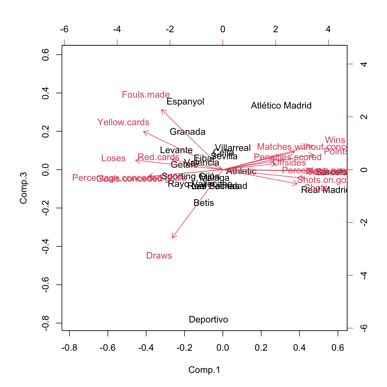

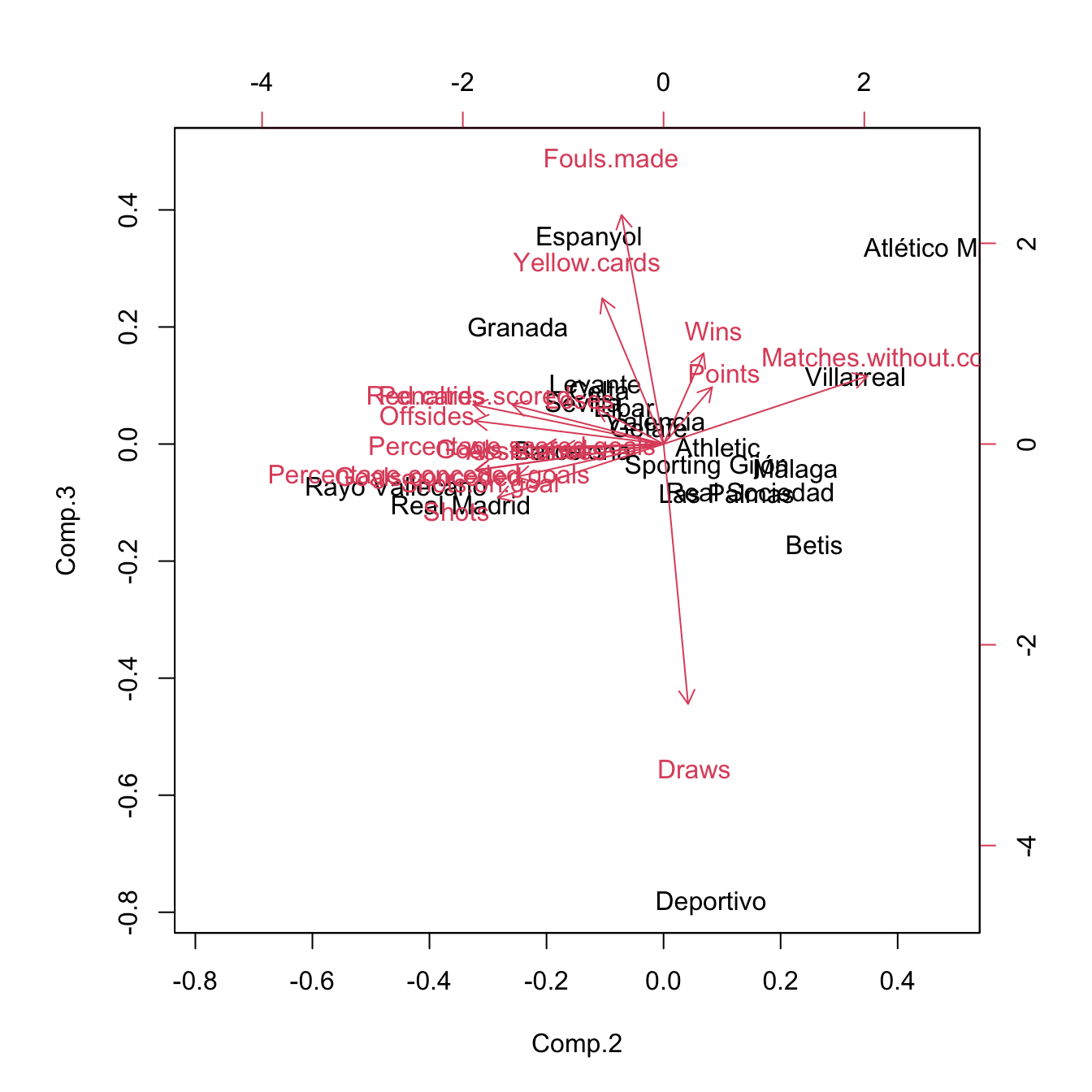
Figure 3.34: Pseudo-biplots for laliga dataset based on principal components 1 and 3, and principal components 2 and 3, respectively.

Exercise 3.14 At the sight of the previous plots, can you think about an interpretation for the third principal component?

3.6.2 Principal components regression

The key idea behind Principal Components Regression (PCR) is to regress the response \(Y\) in a set of principal components \(\Gamma_1,\ldots,\Gamma_\ell\) obtained from the predictors \(X_1,\ldots,X_p,\) where \(\ell<p.\) The motivation is that often a small number of principal components is enough to explain most of the variability of the predictors and consequently their relationship with \(Y.\)⁹² Therefore, we look for fitting the linear model⁹³

\[\begin{align} Y=\alpha_0+\alpha_1\Gamma_1+\cdots+\alpha_\ell\Gamma_\ell+\varepsilon.\tag{3.13} \end{align}\]

The main advantages of PCR are two:

1. Multicollinearity is avoided by design: \(\Gamma_1,\ldots,\Gamma_\ell\) are uncorrelated between them.
2. There are less coefficients to estimate (\(\ell\) instead of \(p\)), hence the accuracy of the estimation increases.

However, keep in mind that PCR affects the linear model in two fundamental ways:

1. Interpretation of the coefficients is not directly related with the predictors, but with the principal components. Hence, the interpretability of a given coefficient in the regression model is tied to the interpretability of the associated principal component.
2. Prediction needs an extra step, since it is required to obtain the scores of the new observations of the predictors.

The first point is elaborated next. The PCR model (3.13) can be seen as a linear model expressed in terms of the original predictors. To make this point clearer, let’s re-express (3.13) as

\[\begin{align} Y=\alpha_0+\boldsymbol{\Gamma}_{1:\ell}^\top\boldsymbol{\alpha}_{1:\ell}+\varepsilon,\tag{3.14} \end{align}\]

where the subindex \(1:\ell\) denotes the inclusion of the vector entries from \(1\) to \(\ell.\) Now, we can express the PCR problem (3.14) in terms of the original predictors:⁹⁴

\[\begin{align*} Y&=\alpha_0+(\mathbf{A}_{1:\ell}^\top(\mathbf{X}-\boldsymbol{\mu}))^\top\boldsymbol{\alpha}_{1:\ell}+\varepsilon\\ &=(\alpha_0-\boldsymbol{\mu}^\top\mathbf{A}_{1:\ell}\boldsymbol{\alpha}_{1:\ell})+\mathbf{X}^\top\mathbf{A}_{1:\ell}\boldsymbol{\alpha}_{1:\ell}+\varepsilon\\ &=\gamma_0+\mathbf{X}^\top\boldsymbol{\gamma}_{1:p}+\varepsilon, \end{align*}\]

where \(\mathbf{A}_{1:\ell}\) represents the \(\mathbf{A}\) matrix with only its first \(\ell\) columns and

\[\begin{align} \gamma_0:=\alpha_0-\boldsymbol{\mu}^\top\mathbf{A}_{1:\ell}\boldsymbol{\alpha}_{1:\ell},\quad \boldsymbol{\gamma}_{1:p}:=\mathbf{A}_{1:\ell}\boldsymbol{\alpha}_{1:\ell}.\tag{3.15} \end{align}\]

In other words, the coefficients \(\boldsymbol{\alpha}_{1:\ell}\) of the PCR done with \(\ell\) principal components in (3.13) translate into the coefficients (3.15) of the linear model based on the \(p\) original predictors:

\[\begin{align*} Y=\gamma_0+\gamma_1X_1+\cdots+\gamma_pX_p+\varepsilon. \end{align*}\]

In the sample case, we have that

\[\begin{align} \hat{\gamma}_0=\hat\alpha_0-\bar{\mathbf{X}}^\top\hat{\mathbf{A}}_{1:\ell}\hat{\boldsymbol{\alpha}}_{1:\ell},\quad \hat{\boldsymbol{\gamma}}_{1:p}=\hat{\mathbf{A}}_{1:\ell}\hat{\boldsymbol{\alpha}}_{1:\ell}.\tag{3.16} \end{align}\]

Notice that \(\hat{\boldsymbol{\gamma}}\) is not the least squares estimator performed with the original predictors, that we denote by \(\hat{\boldsymbol{\beta}}.\) \(\hat{\boldsymbol{\gamma}}\) contains the coefficients of the PCR that are associated to the original predictors. Consequently, \(\hat{\boldsymbol{\gamma}}\) is useful for the interpretation of the linear model produced by PCR, as it can be interpreted in the same way \(\hat{\boldsymbol{\beta}}\) was.⁹⁵

Finally, remember that the usefulness of PCR relies on how well we are able to reduce the dimensionality⁹⁶ of the predictors and the veracity of the assumption that the \(\ell\) principal components are related with \(Y.\)

Keep in mind that PCR considers the PCA done in the set of predictors, that is, we exclude the response for obvious reasons (a perfect and useless fit). It is important to remove the response from the call to princomp if we want to use the output in lm.

We see now two approaches for performing PCR, which we illustrate with the laliga dataset. The common objective is to predict Points using the remaining variables (excluding those directly related: Wins, Draws, Loses, and Matches.without.conceding) in order to quantify, explain, and predict the final points of a team from its performance.

The first approach combines the use of the princomp and lm functions. Its strong points are that it is both able to predict and explain, and is linked with techniques we have employed so far. The weak point is that it requires extra coding.

# A linear model is problematic
mod <- lm(Points ~ . - Wins - Draws - Loses - Matches.without.conceding,
          data = laliga)
summary(mod) # Lots of non-significant predictors
## 
## Call:
## lm(formula = Points ~ . - Wins - Draws - Loses - Matches.without.conceding, 
##     data = laliga)
## 
## Residuals:
##     Min      1Q  Median      3Q     Max 
## -5.2117 -1.4766  0.0544  1.9515  4.1422 
## 
## Coefficients:
##                             Estimate Std. Error t value Pr(>|t|)  
## (Intercept)                 77.11798   26.12915   2.951   0.0214 *
## Goals.scored               -28.21714   17.44577  -1.617   0.1498  
## Goals.conceded             -24.23628   15.45595  -1.568   0.1608  
## Percentage.scored.goals   1066.98731  655.69726   1.627   0.1477  
## Percentage.conceded.goals  896.94781  584.97833   1.533   0.1691  
## Shots                       -0.10246    0.07754  -1.321   0.2279  
## Shots.on.goal                0.02024    0.13656   0.148   0.8863  
## Penalties.scored            -0.81018    0.77600  -1.044   0.3312  
## Assistances                  1.41971    0.44103   3.219   0.0147 *
## Fouls.made                  -0.04438    0.04267  -1.040   0.3328  
## Yellow.cards                 0.27850    0.16814   1.656   0.1416  
## Red.cards                    0.68663    1.44229   0.476   0.6485  
## Offsides                    -0.00486    0.14854  -0.033   0.9748  
## ---
## Signif. codes:  0 '***' 0.001 '**' 0.01 '*' 0.05 '.' 0.1 ' ' 1
## 
## Residual standard error: 4.274 on 7 degrees of freedom
## Multiple R-squared:  0.9795, Adjusted R-squared:  0.9443 
## F-statistic: 27.83 on 12 and 7 DF,  p-value: 9.784e-05

# We try to clean the model
modBIC <- MASS::stepAIC(mod, k = log(nrow(laliga)), trace = 0)
summary(modBIC) # Better, but still unsatisfactory
## 
## Call:
## lm(formula = Points ~ Goals.scored + Goals.conceded + Percentage.scored.goals + 
##     Percentage.conceded.goals + Shots + Assistances + Yellow.cards, 
##     data = laliga)
## 
## Residuals:
##     Min      1Q  Median      3Q     Max 
## -5.4830 -1.4505  0.9008  1.1813  5.8662 
## 
## Coefficients:
##                            Estimate Std. Error t value Pr(>|t|)    
## (Intercept)                62.91373   10.73528   5.860 7.71e-05 ***
## Goals.scored              -23.90903   11.22573  -2.130  0.05457 .  
## Goals.conceded            -12.16610    8.11352  -1.499  0.15959    
## Percentage.scored.goals   894.56861  421.45891   2.123  0.05528 .  
## Percentage.conceded.goals 440.76333  307.38671   1.434  0.17714    
## Shots                      -0.05752    0.02713  -2.120  0.05549 .  
## Assistances                 1.42267    0.28462   4.999  0.00031 ***
## Yellow.cards                0.11313    0.07868   1.438  0.17603    
## ---
## Signif. codes:  0 '***' 0.001 '**' 0.01 '*' 0.05 '.' 0.1 ' ' 1
## 
## Residual standard error: 3.743 on 12 degrees of freedom
## Multiple R-squared:  0.973,  Adjusted R-squared:  0.9572 
## F-statistic: 61.77 on 7 and 12 DF,  p-value: 1.823e-08

# Also, huge multicollinearity
car::vif(modBIC)
##              Goals.scored            Goals.conceded   Percentage.scored.goals Percentage.conceded.goals 
##              77998.044760              22299.952547              76320.612579              22322.307151 
##                     Shots               Assistances              Yellow.cards 
##                  6.505748                 32.505831                  3.297224

# A quick way of removing columns without knowing its position
laligaRed <- subset(laliga, select = -c(Points, Wins, Draws, Loses,
                                        Matches.without.conceding))
# PCA without Points, Wins, Draws, Loses, and Matches.without.conceding
pcaLaligaRed <- princomp(x = laligaRed, cor = TRUE, fix_sign = TRUE)
summary(pcaLaligaRed) # l = 3 gives 86% of variance explained
## Importance of components:
##                           Comp.1    Comp.2     Comp.3    Comp.4     Comp.5    Comp.6      Comp.7      Comp.8
## Standard deviation     2.7437329 1.4026745 0.91510249 0.8577839 0.65747209 0.5310954 0.332556029 0.263170555
## Proportion of Variance 0.6273392 0.1639580 0.06978438 0.0613161 0.03602246 0.0235052 0.009216126 0.005771562
## Cumulative Proportion  0.6273392 0.7912972 0.86108155 0.9223977 0.95842012 0.9819253 0.991141438 0.996913000
##                             Comp.9     Comp.10      Comp.11      Comp.12
## Standard deviation     0.146091551 0.125252621 3.130311e-03 1.801036e-03
## Proportion of Variance 0.001778562 0.001307352 8.165704e-07 2.703107e-07
## Cumulative Proportion  0.998691562 0.999998913 9.999997e-01 1.000000e+00

# Interpretation of PC1 and PC2
biplot(pcaLaligaRed)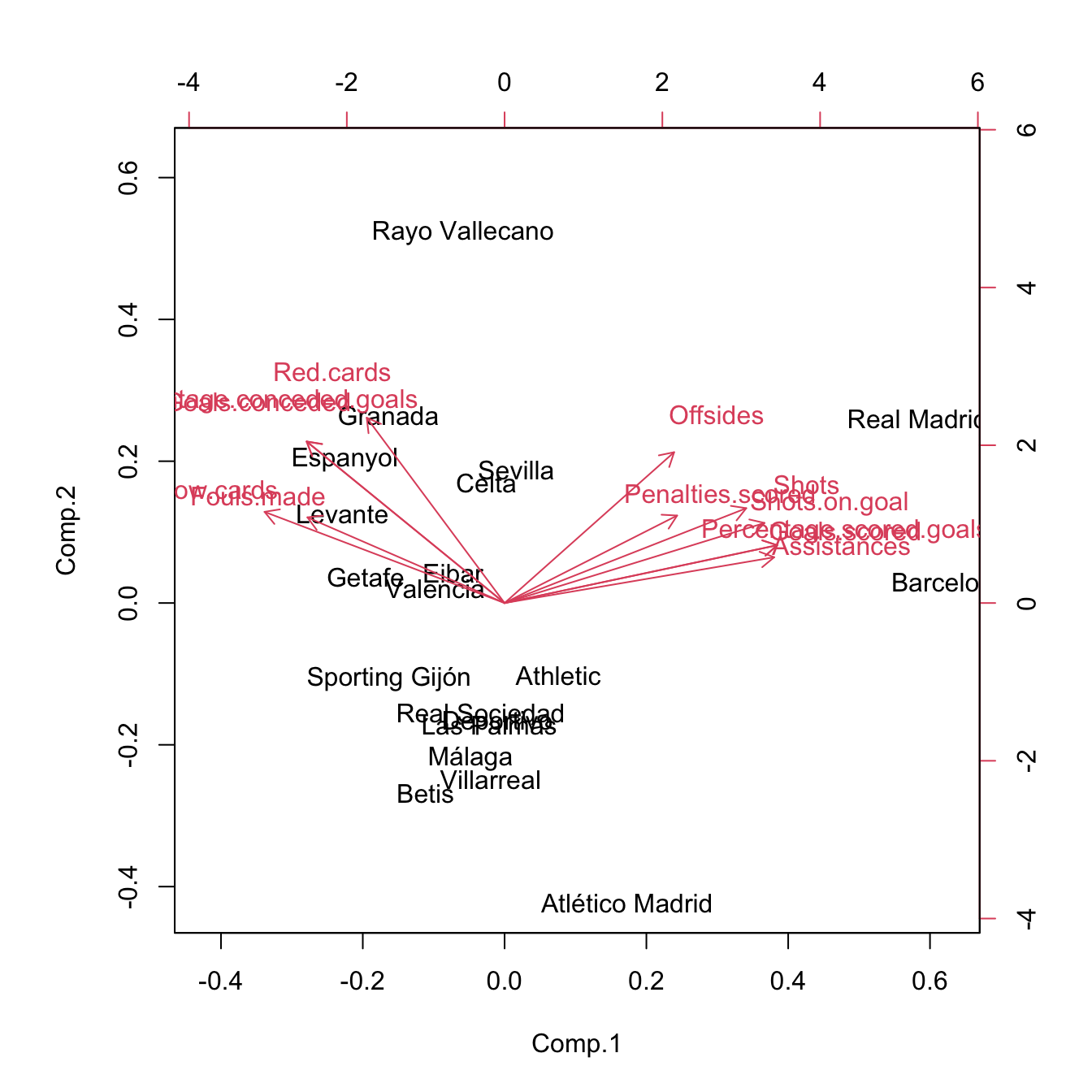

# PC1: attack performance of the team

# Create a new dataset with the response + principal components
laligaPCA <- data.frame("Points" = laliga$Points, pcaLaligaRed$scores)

# Regression on all the principal components
modPCA <- lm(Points ~ ., data = laligaPCA)
summary(modPCA) # Predictors clearly significant -- same R^2 as mod
## 
## Call:
## lm(formula = Points ~ ., data = laligaPCA)
## 
## Residuals:
##     Min      1Q  Median      3Q     Max 
## -5.2117 -1.4766  0.0544  1.9515  4.1422 
## 
## Coefficients:
##              Estimate Std. Error t value Pr(>|t|)    
## (Intercept)   52.4000     0.9557  54.831 1.76e-10 ***
## Comp.1         5.7690     0.3483  16.563 7.14e-07 ***
## Comp.2        -2.4376     0.6813  -3.578   0.0090 ** 
## Comp.3         3.4222     1.0443   3.277   0.0135 *  
## Comp.4        -3.6079     1.1141  -3.238   0.0143 *  
## Comp.5         1.9713     1.4535   1.356   0.2172    
## Comp.6         5.7067     1.7994   3.171   0.0157 *  
## Comp.7        -3.4169     2.8737  -1.189   0.2732    
## Comp.8         9.0212     3.6313   2.484   0.0419 *  
## Comp.9        -4.6455     6.5415  -0.710   0.5006    
## Comp.10      -10.2087     7.6299  -1.338   0.2227    
## Comp.11      222.0340   305.2920   0.727   0.4907    
## Comp.12     -954.7650   530.6164  -1.799   0.1150    
## ---
## Signif. codes:  0 '***' 0.001 '**' 0.01 '*' 0.05 '.' 0.1 ' ' 1
## 
## Residual standard error: 4.274 on 7 degrees of freedom
## Multiple R-squared:  0.9795, Adjusted R-squared:  0.9443 
## F-statistic: 27.83 on 12 and 7 DF,  p-value: 9.784e-05
car::vif(modPCA) # No problems at all
##  Comp.1  Comp.2  Comp.3  Comp.4  Comp.5  Comp.6  Comp.7  Comp.8  Comp.9 Comp.10 Comp.11 Comp.12 
##       1       1       1       1       1       1       1       1       1       1       1       1

# Using the first three components
modPCA3 <- lm(Points ~ Comp.1 + Comp.2 + Comp.3, data = laligaPCA)
summary(modPCA3)
## 
## Call:
## lm(formula = Points ~ Comp.1 + Comp.2 + Comp.3, data = laligaPCA)
## 
## Residuals:
##    Min     1Q Median     3Q    Max 
## -8.178 -4.541 -1.401  3.501 16.093 
## 
## Coefficients:
##             Estimate Std. Error t value Pr(>|t|)    
## (Intercept)  52.4000     1.5672  33.435 3.11e-16 ***
## Comp.1        5.7690     0.5712  10.100 2.39e-08 ***
## Comp.2       -2.4376     1.1173  -2.182   0.0444 *  
## Comp.3        3.4222     1.7126   1.998   0.0630 .  
## ---
## Signif. codes:  0 '***' 0.001 '**' 0.01 '*' 0.05 '.' 0.1 ' ' 1
## 
## Residual standard error: 7.009 on 16 degrees of freedom
## Multiple R-squared:  0.8738, Adjusted R-squared:  0.8501 
## F-statistic: 36.92 on 3 and 16 DF,  p-value: 2.027e-07

# Coefficients associated with each original predictor (gamma)
alpha <- modPCA3$coefficients
gamma <- pcaLaligaRed$loadings[, 1:3] %*% alpha[-1] # Slopes
gamma <- c(alpha[1] - pcaLaligaRed$center %*% gamma, gamma) # Intercept
names(gamma) <- c("Intercept", rownames(pcaLaligaRed$loadings))
gamma
##                 Intercept              Goals.scored            Goals.conceded   Percentage.scored.goals 
##               -44.2288551                 1.7305124                -3.4048178                 1.7416378 
## Percentage.conceded.goals                     Shots             Shots.on.goal          Penalties.scored 
##                -3.3944235                 0.2347716                 0.8782162                 2.6044699 
##               Assistances                Fouls.made              Yellow.cards                 Red.cards 
##                 1.4548813                -0.1171732                -1.7826488                -2.6423211 
##                  Offsides 
##                 1.3755697

# We can overpenalize to have a simpler model -- also one single
# principal component does quite well
modPCABIC <- MASS::stepAIC(modPCA, k = 2 * log(nrow(laliga)), trace = 0)
summary(modPCABIC)
## 
## Call:
## lm(formula = Points ~ Comp.1 + Comp.2 + Comp.3 + Comp.4 + Comp.6 + 
##     Comp.8, data = laligaPCA)
## 
## Residuals:
##     Min      1Q  Median      3Q     Max 
## -6.6972 -2.6418 -0.3265  2.3535  8.4944 
## 
## Coefficients:
##             Estimate Std. Error t value Pr(>|t|)    
## (Intercept)  52.4000     1.0706  48.946 3.95e-16 ***
## Comp.1        5.7690     0.3902  14.785 1.65e-09 ***
## Comp.2       -2.4376     0.7632  -3.194  0.00705 ** 
## Comp.3        3.4222     1.1699   2.925  0.01182 *  
## Comp.4       -3.6079     1.2481  -2.891  0.01263 *  
## Comp.6        5.7067     2.0158   2.831  0.01416 *  
## Comp.8        9.0212     4.0680   2.218  0.04502 *  
## ---
## Signif. codes:  0 '***' 0.001 '**' 0.01 '*' 0.05 '.' 0.1 ' ' 1
## 
## Residual standard error: 4.788 on 13 degrees of freedom
## Multiple R-squared:  0.9521, Adjusted R-squared:  0.9301 
## F-statistic: 43.11 on 6 and 13 DF,  p-value: 7.696e-08
# Note that the order of the principal components does not correspond
# exactly to its importance in the regression!

# To perform prediction we need to compute first the scores associated to the
# new values of the predictors, conveniently preprocessed
# Predictions for FCB and RMA (although they are part of the training sample)
newPredictors <- laligaRed[1:2, ]
newPredictors <- scale(newPredictors, center = pcaLaligaRed$center,
                       scale = pcaLaligaRed$scale) # Centered and scaled
newScores <- t(apply(newPredictors, 1,
                     function(x) t(pcaLaligaRed$loadings) %*% x))

# We need a data frame for prediction
newScores <- data.frame("Comp" = newScores)
predict(modPCABIC, newdata = newScores, interval = "prediction")
##                  fit      lwr      upr
## Barcelona   93.64950 80.35115 106.9478
## Real Madrid 90.05622 77.11876 102.9937

# Reality
laliga[1:2, 1]
## [1] 91 90

The second approach employs the function pls::pcr and is more direct, yet less connected with the techniques we have seen so far. It employs a model object that is different from the lm object and, as a consequence, functions like summary, BIC, MASS::stepAIC, or plot will not work properly. This implies that inference, model selection, and model diagnostics are not so straightforward. In exchange, pls::pcr allows for model fitting in an easier way and model selection through the use of cross-validation. In overall, this is a more pure predictive approach than predictive and explicative.

# Create a dataset without the problematic predictors and with the response
laligaRed2 <- subset(laliga, select = -c(Wins, Draws, Loses,
                                         Matches.without.conceding))

# Simple call to pcr
library(pls)
modPcr <- pcr(Points ~ ., data = laligaRed2, scale = TRUE)
# Notice we do not need to create a data.frame with PCA, it is automatically
# done within pcr. We also have flexibility to remove predictors from the PCA
# scale = TRUE means that the predictors are scaled internally before computing
# PCA

# The summary of the model is different
summary(modPcr)
## Data:    X dimension: 20 12 
##  Y dimension: 20 1
## Fit method: svdpc
## Number of components considered: 12
## TRAINING: % variance explained
##         1 comps  2 comps  3 comps  4 comps  5 comps  6 comps  7 comps  8 comps  9 comps  10 comps  11 comps  12 comps
## X         62.73    79.13    86.11    92.24    95.84    98.19    99.11    99.69    99.87    100.00       100    100.00
## Points    80.47    84.23    87.38    90.45    90.99    93.94    94.36    96.17    96.32     96.84        97     97.95
# First row: percentage of variance explained of the predictors
# Second row: percentage of variance explained of Y (the R^2)
# Note that we have the same R^2 for 3 and 12 components as in the previous
# approach

# Slots of information in the model -- most of them as 3-dim arrays with the
# third dimension indexing the number of components considered
names(modPcr)
##  [1] "coefficients"  "scores"        "loadings"      "Yloadings"     "projection"    "Xmeans"        "Ymeans"       
##  [8] "fitted.values" "residuals"     "Xvar"          "Xtotvar"       "fit.time"      "ncomp"         "method"       
## [15] "center"        "scale"         "call"          "terms"         "model"

# The coefficients of the original predictors (gammas), not of the components!
modPcr$coefficients[, , 12]
##              Goals.scored            Goals.conceded   Percentage.scored.goals Percentage.conceded.goals 
##             -602.85050765             -383.07010184              600.61255371              374.38729000 
##                     Shots             Shots.on.goal          Penalties.scored               Assistances 
##               -8.27239221                0.88174787               -2.14313238               24.42240486 
##                Fouls.made              Yellow.cards                 Red.cards                  Offsides 
##               -2.96044265                5.51983512                1.20945331               -0.07231723
# pcr() computes up to ncomp (in this case, 12) linear models, each one
# considering one extra principal component. $coefficients returns in a
# 3-dim array the coefficients of all the linear models

# Prediction is simpler and can be done for different number of components
predict(modPcr, newdata = laligaRed2[1:2, ], ncomp = 12)
## , , 12 comps
## 
##               Points
## Barcelona   92.01244
## Real Madrid 91.38026

# Selecting the number of components to retain. All the components up to ncomp
# are selected, no further flexibility is possible
modPcr2 <- pcr(Points ~ ., data = laligaRed2, scale = TRUE, ncomp = 3)
summary(modPcr2)
## Data:    X dimension: 20 12 
##  Y dimension: 20 1
## Fit method: svdpc
## Number of components considered: 3
## TRAINING: % variance explained
##         1 comps  2 comps  3 comps
## X         62.73    79.13    86.11
## Points    80.47    84.23    87.38

# Selecting the number of components to retain by Leave-One-Out
# cross-validation
modPcrCV1 <- pcr(Points ~ ., data = laligaRed2, scale = TRUE,
                 validation = "LOO")
summary(modPcrCV1)
## Data:    X dimension: 20 12 
##  Y dimension: 20 1
## Fit method: svdpc
## Number of components considered: 12
## 
## VALIDATION: RMSEP
## Cross-validated using 20 leave-one-out segments.
##        (Intercept)  1 comps  2 comps  3 comps  4 comps  5 comps  6 comps  7 comps  8 comps  9 comps  10 comps  11 comps
## CV           18.57    8.505    8.390    8.588    7.571    7.688    6.743     7.09    6.224    6.603     7.547     8.375
## adjCV        18.57    8.476    8.356    8.525    7.513    7.663    6.655     7.03    6.152    6.531     7.430     8.236
##        12 comps
## CV        7.905
## adjCV     7.760
## 
## TRAINING: % variance explained
##         1 comps  2 comps  3 comps  4 comps  5 comps  6 comps  7 comps  8 comps  9 comps  10 comps  11 comps  12 comps
## X         62.73    79.13    86.11    92.24    95.84    98.19    99.11    99.69    99.87    100.00       100    100.00
## Points    80.47    84.23    87.38    90.45    90.99    93.94    94.36    96.17    96.32     96.84        97     97.95

# View cross-validation Mean Squared Error in Prediction
validationplot(modPcrCV1, val.type = "MSEP") # l = 8 gives the minimum CV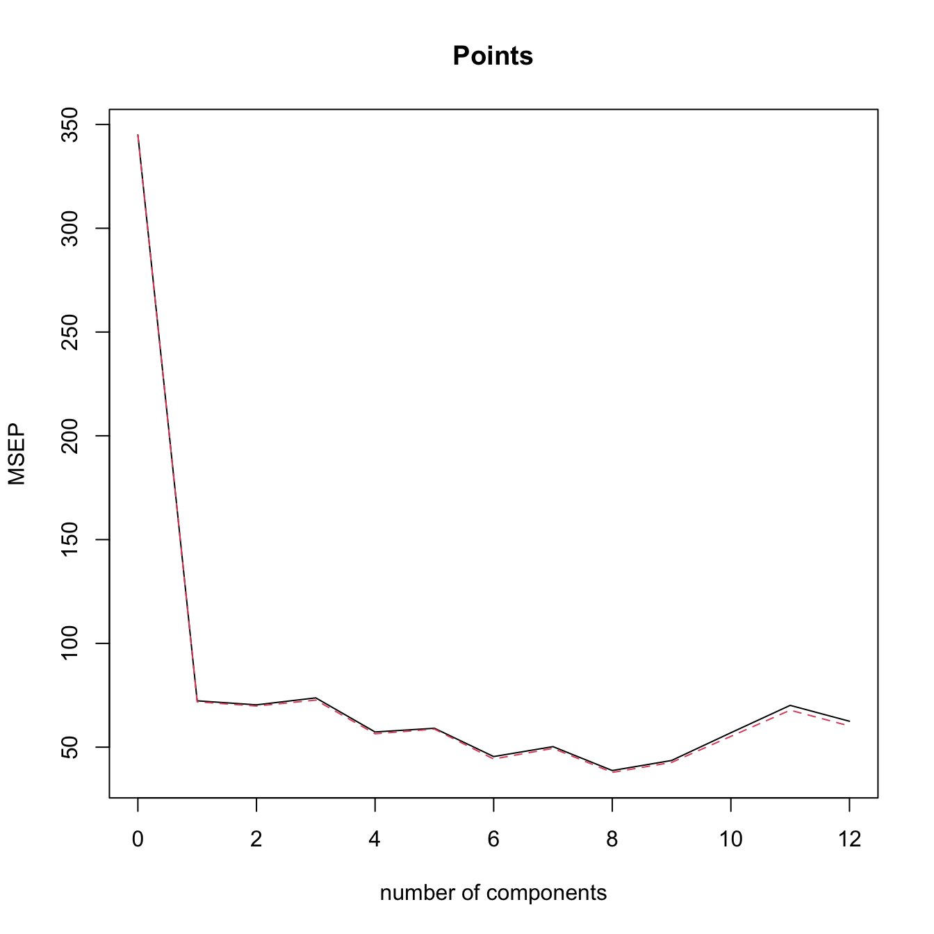

# The black is the CV loss, the dashed red line is the adjCV loss, a bias
# corrected version of the MSEP (not described in the notes)

# Selecting the number of components to retain by 10-fold Cross-Validation
# (k = 10 is the default, this can be changed with the argument segments)
modPcrCV10 <- pcr(Points ~ ., data = laligaRed2, scale = TRUE,
                  validation = "CV")
summary(modPcrCV10)
## Data:    X dimension: 20 12 
##  Y dimension: 20 1
## Fit method: svdpc
## Number of components considered: 12
## 
## VALIDATION: RMSEP
## Cross-validated using 10 random segments.
##        (Intercept)  1 comps  2 comps  3 comps  4 comps  5 comps  6 comps  7 comps  8 comps  9 comps  10 comps  11 comps
## CV           18.57    8.520    8.392    8.911    7.187    7.124    6.045    6.340    5.728    6.073     7.676     9.300
## adjCV        18.57    8.464    8.331    8.768    7.092    7.043    5.904    6.252    5.608    5.953     7.423     8.968
##        12 comps
## CV        9.151
## adjCV     8.782
## 
## TRAINING: % variance explained
##         1 comps  2 comps  3 comps  4 comps  5 comps  6 comps  7 comps  8 comps  9 comps  10 comps  11 comps  12 comps
## X         62.73    79.13    86.11    92.24    95.84    98.19    99.11    99.69    99.87    100.00       100    100.00
## Points    80.47    84.23    87.38    90.45    90.99    93.94    94.36    96.17    96.32     96.84        97     97.95
validationplot(modPcrCV10, val.type = "MSEP") # l = 8 gives the minimum CV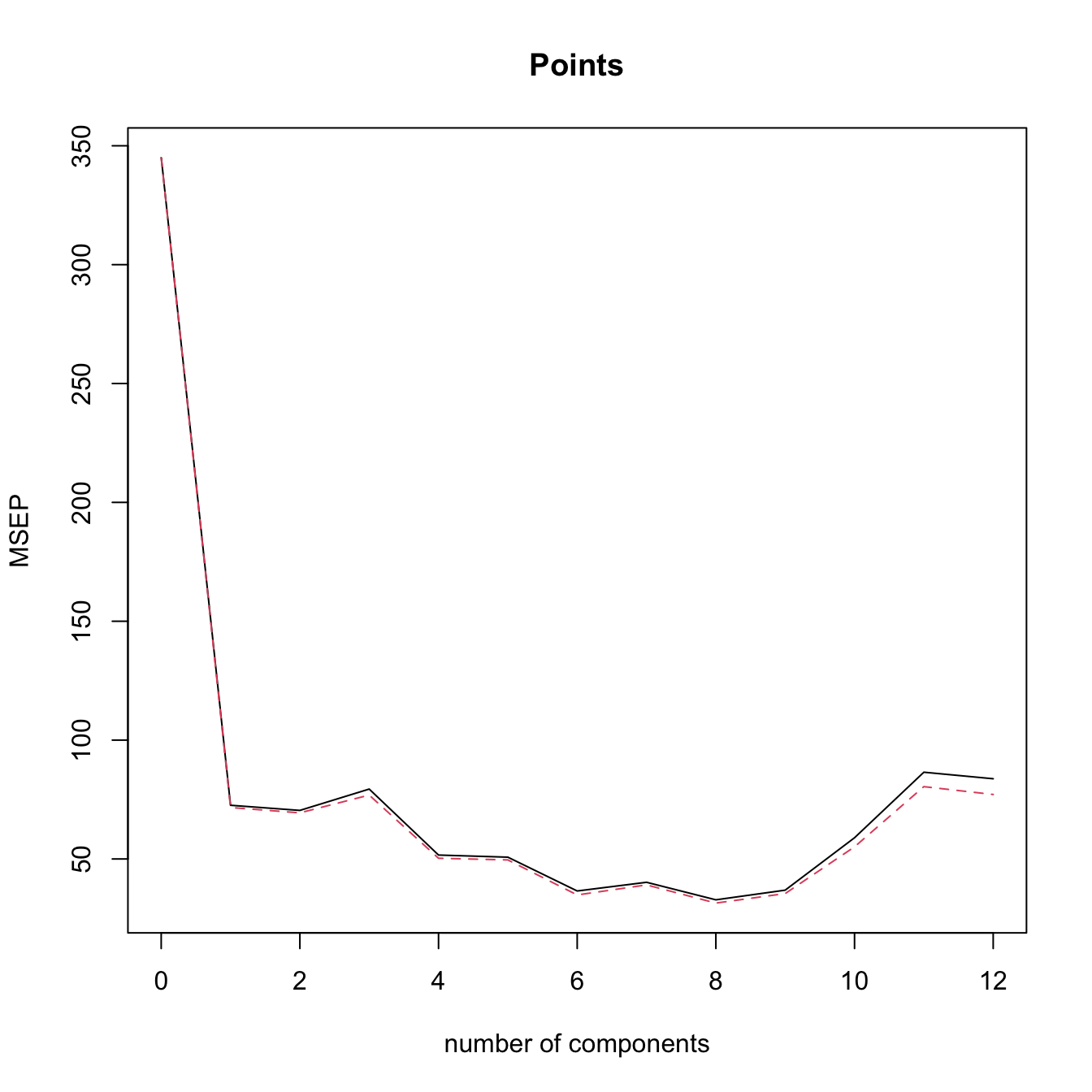

pcr() does an internal scaling of the predictors by their quasi-standard deviations. This means that each variable is divided by \(\frac{1}{\sqrt{n-1}},\) when in princomp a scaling of \(\frac{1}{\sqrt{n}}\) is applied (the standard deviations are employed). This results in a minor discrepancy in the scores object of both methods that is easily patchable. The scores of princomp() are the ones of pcr() multiplied by \(\sqrt{\frac{n}{n-1}}.\) This problem is inherited to the coefficients, which assume scores divided by \(\frac{1}{\sqrt{n-1}}.\) Therefore, the \(\hat{\boldsymbol{\gamma}}\) coefficients described in (3.16) are obtained by dividing the coefficients of pcr() by \(\sqrt{\frac{n}{n-1}}.\)

The next chunk of code illustrates the previous warning.

# Equality of loadings from princomp() and pcr()
max(abs(abs(pcaLaligaRed$loadings[, 1:3]) - abs(modPcr$loadings[, 1:3])))
## [1] 2.664535e-15

# Equality of scores from princomp() and pcr() (with the same standardization)
max(abs(abs(pcaLaligaRed$scores[, 1:3]) -
          abs(modPcr$scores[, 1:3] * sqrt(n / (n - 1)))))
## [1] 9.298118e-15

# Equality of the gamma coefficients obtained previously for 3 PCA
# (with the same standardization)
modPcr$coefficients[, , 3] / sqrt(n / (n - 1))
##              Goals.scored            Goals.conceded   Percentage.scored.goals Percentage.conceded.goals 
##                 1.7305124                -3.4048178                 1.7416378                -3.3944235 
##                     Shots             Shots.on.goal          Penalties.scored               Assistances 
##                 0.2347716                 0.8782162                 2.6044699                 1.4548813 
##                Fouls.made              Yellow.cards                 Red.cards                  Offsides 
##                -0.1171732                -1.7826488                -2.6423211                 1.3755697
gamma[-1]
##              Goals.scored            Goals.conceded   Percentage.scored.goals Percentage.conceded.goals 
##                 1.7305124                -3.4048178                 1.7416378                -3.3944235 
##                     Shots             Shots.on.goal          Penalties.scored               Assistances 
##                 0.2347716                 0.8782162                 2.6044699                 1.4548813 
##                Fouls.made              Yellow.cards                 Red.cards                  Offsides 
##                -0.1171732                -1.7826488                -2.6423211                 1.3755697

# Coefficients associated with the principal components -- same as in modPCA3
lm(Points ~ ., data = data.frame("Points" = laliga$Points,
                                 modPcr$scores[, 1:3] * sqrt(n / (n - 1))))
## 
## Call:
## lm(formula = Points ~ ., data = data.frame(Points = laliga$Points, 
##     modPcr$scores[, 1:3] * sqrt(n/(n - 1))))
## 
## Coefficients:
## (Intercept)       Comp.1       Comp.2       Comp.3  
##      52.400       -5.769        2.438       -3.422
modPCA3
## 
## Call:
## lm(formula = Points ~ Comp.1 + Comp.2 + Comp.3, data = laligaPCA)
## 
## Coefficients:
## (Intercept)       Comp.1       Comp.2       Comp.3  
##      52.400        5.769       -2.438        3.422
# Of course, flipping of signs is always possible with PCA

The selection of \(\ell\) by cross-validation attempts to minimize the Mean Squared Error in Prediction (MSEP) or, equivalently, the Root MSEP (RMSEP) of the model.⁹⁷ This is a Swiss army knife method valid for the selection of any tuning parameter \(\lambda\) that affects the form of the estimate \(\hat{m}_\lambda\) of the regression function \(m\) (remember (1.1)). Given the sample \(\{(\mathbf{X}_i,Y_i)\}_{i=1}^n,\) leave-one-out cross-validation considers the tuning parameter

\[\begin{align} \hat{\lambda}_\text{CV}:=\arg\min_{\lambda\geq0} \sum_{i=1}^n (Y_i-\hat{m}_{\lambda,-i}(\mathbf{X}_i))^2,\tag{3.17} \end{align}\]

where \(\hat{m}_{\lambda,-i}\) represents the fit of the model \(\hat{m}_\lambda\) without the \(i\)-th observation \((\mathbf{X}_i,Y_i).\)

A less computationally expensive variation on leave-one-out cross-validation is \(k\)-fold cross-validation, which partitions the data into \(k\) folds \(F_1,\ldots, F_k\) of approximately equal size, trains the model \(\hat{m}_\lambda\) in the aggregation of \(k-1\) folds, and evaluates its MSEP in the remaining fold:

\[\begin{align} \hat{\lambda}_{k\text{-CV}}:=\arg\min_{\lambda\geq0} \sum_{j=1}^k \sum_{i\in F_j} (Y_i-\hat{m}_{\lambda,-F_{j}}(\mathbf{X}_i))^2,\tag{3.18} \end{align}\]

where \(\hat{m}_{\lambda,-F_{j}}\) represents the fit of the model \(\hat{m}_\lambda\) excluding the data from the \(j\)-th fold \(F_{j}.\) Recall that \(k\)-fold cross-validation is more general than leave-one-out cross-validation, since the latter is a particular case of the former with \(k=n.\)

\(k\)-fold cross validation with \(k<n\) depends on the choice of the folds for splitting the data (i.e., how each datum is assigned to each of the \(k\) folds). Some statistical softwares do this assignment randomly, which means that the selection of \(\hat{\lambda}_{k\text{-CV}}\) may vary from one run to another. Thus, fixing the seed prior to the parameter selection is important to ensure reproducibility. Another alternative is to aggregate, in a convenient way, the results of several \(k\)-fold cross-validations done in different random partitions. This problem is not present in leave-one-out cross-validation (where \(k=n\)).

Inference in PCR can be carried out as in the standard linear model. The key point is to realize that it is about the coefficients \(\boldsymbol{\alpha}_{0:\ell}\) associated with the \(\ell\) principal components, and that it can be carried out by the summary() function on the output of lm(). The coefficients \(\boldsymbol{\alpha}_{0:\ell}\) are the ones estimated by least squares when considering the scores of the \(\ell\) principal components as the predictors. This transformation of the predictors does not affect the validity of the inferential results of Section 2.4 (derived conditionally on the predictors). But recall that this inference is not about \(\boldsymbol{\gamma}.\)

Inference in PCR is based on the assumptions of the linear model being satisfied for the considered principal components. The evaluation of the assumptions can be done using the exact same tools described in Section 3.5. However, keep in mind that PCA is a linear transformation of the data. Therefore:

• If the linearity assumption fails for the predictors \(X_1,\ldots,X_p,\) then it will also likely fail for \(\Gamma_1,\ldots,\Gamma_\ell,\) since the transformation will not introduce nonlinearities able to capture the nonlinear effects.
• Similarly, if the homoscedasticity, normality, or independence assumptions fail for \(X_1,\ldots,X_p,\) then they will also likely fail for \(\Gamma_1,\ldots,\Gamma_\ell.\)

Exceptions to the previous common implications are possible, and may involve the association of one or several problematic predictors (e.g., have nonlinear effects on the response) to the principal components that are excluded from the model. Up to which extent the failure of the assumptions in the original predictors can be mitigated by PCR depends on each application.

3.6.3 Partial least squares regression

PCR works by replacing the predictors \(X_1,\ldots,X_p\) by a set of principal components \(\Gamma_1,\ldots,\Gamma_\ell,\) under the hope that these directions, that explain most of the variability of the predictors, are also the best directions for predicting the response \(Y.\) While this is a reasonable belief, it is not a guaranteed fact. Partial Least Squares Regression (PLSR) precisely tackles this point with the idea of regressing the response \(Y\) on a set of new variables \(P_1,\ldots,P_\ell\) that are constructed with the objective of predicting \(Y\) from \(X_1,\ldots,X_p\) in the best linear way.

As with PCA, the idea is to find linear combinations of the predictors \(X_1,\ldots,X_p,\) that is, to have:

\[\begin{align} P_1:=\sum_{j=1}^pa_{1j}X_j,\,\ldots,\,P_p:=\sum_{j=1}^pa_{pj}X_j.\tag{3.19} \end{align}\]

These new predictors are called PLS components.⁹⁸

The question is how to choose the coefficients \(a_{kj},\) \(j,k=1,\ldots,p.\) PLSR does it by placing the most weight in the predictors that are most strongly correlated with \(Y\) and in such a way that the resulting \(P_1,\ldots,P_p\) are uncorrelated between them. After standardizing the variables, for \(P_1\) this is achieved by setting \(a_{1j}\) equal to the theoretical slope coefficient of regressing \(Y\) into \(X_j,\) that is:⁹⁹

\[\begin{align*} a_{1j}:=\frac{\mathrm{Cov}[X_j,Y]}{\mathbb{V}\mathrm{ar}[X_j]}, \end{align*}\]

where \(a_{1j}\) stems from \(Y=a_{0}+a_{1j}X_j+\varepsilon.\)

The second partial least squares direction, \(P_2,\) is computed in a similar way, but once the linear effects of \(P_1\) on \(X_1,\ldots,X_p\) are removed. This is achieved by:

1. Regressing each of \(X_1,\ldots,X_p\) on \(P_1.\) That is, fit the \(p\) simple linear models

\[\begin{align*} X_j=\alpha_0+\alpha_{1j}P_1+\varepsilon_j,\quad j=1,\ldots,p. \end{align*}\]

2. Regress \(Y\) on each of the \(p\) random errors \(\varepsilon_{1},\ldots,\varepsilon_{p}\;\)¹⁰⁰ from the above regressions, yielding

   \[\begin{align*} a_{2j}:=\frac{\mathrm{Cov}[\varepsilon_j,Y]}{\mathbb{V}\mathrm{ar}[\varepsilon_j]}, \end{align*}\]

   where \(a_{2j}\) stems from \(Y=a_{0}+a_{2j}\varepsilon_j+\varepsilon.\)

The coefficients for \(P_j,\) \(j>2,\) are computed¹⁰¹ by iterating the former process. Once \(P_1,\ldots,P_\ell\) are obtained, then PLSR proceeds as PCR and fits the model

\[\begin{align*} Y=\beta_0+\beta_1P_1+\cdots+\beta_\ell P_\ell+\varepsilon. \end{align*}\]

The implementation of PLSR can be done by the function pls::plsr, which has an analogous syntax to pls::pcr.

# Simple call to plsr -- very similar to pcr
modPlsr <- plsr(Points ~ ., data = laligaRed2, scale = TRUE)

# The summary of the model
summary(modPlsr)
## Data:    X dimension: 20 12 
##  Y dimension: 20 1
## Fit method: kernelpls
## Number of components considered: 12
## TRAINING: % variance explained
##         1 comps  2 comps  3 comps  4 comps  5 comps  6 comps  7 comps  8 comps  9 comps  10 comps  11 comps  12 comps
## X         62.53    76.07    84.94    88.29    92.72    95.61    98.72    99.41    99.83    100.00    100.00    100.00
## Points    83.76    91.06    93.93    95.43    95.94    96.44    96.55    96.73    96.84     96.84     97.69     97.95
# First row: percentage of variance explained of the predictors
# Second row: percentage of variance explained of Y (the R^2)
# Note we have the same R^2 for 12 components as in the linear model

# Slots of information in the model
names(modPlsr)
##  [1] "coefficients"    "scores"          "loadings"        "loading.weights" "Yscores"         "Yloadings"      
##  [7] "projection"      "Xmeans"          "Ymeans"          "fitted.values"   "residuals"       "Xvar"           
## [13] "Xtotvar"         "fit.time"        "ncomp"           "method"          "center"          "scale"          
## [19] "call"            "terms"           "model"

# PLS scores
head(modPlsr$scores)
##                      Comp 1     Comp 2     Comp 3     Comp 4     Comp 5      Comp 6     Comp 7     Comp 8      Comp 9
## Barcelona        7.36407868 -0.6592285 -0.4262822 -0.1357589  0.8668796 -0.52701770 -0.1547704 -0.3104798 -0.15841110
## Real Madrid      6.70659816 -1.2848902  0.7191143  0.5679398 -0.5998745  0.30663290  0.5382173  0.2110337  0.15242836
## Atlético Madrid  2.45577740  2.6469837  0.4573647  0.6179274 -0.4307465  0.13368949  0.2951566 -0.1597672 -0.15232469
## Villarreal       0.06913485  2.0275895  0.6548014 -0.2358589  0.8350426  0.61305618 -0.6684330  0.0556628  0.07919102
## Athletic         0.96513341  0.3860060 -0.2718465 -0.1580349 -0.2649106  0.01822319 -0.1899969  0.3846156 -0.28926416
## Celta           -0.39588401 -0.5296417  0.6148093  0.1494496  0.5817902  0.69106828  0.1586472  0.2396975  0.41575546
##                     Comp 10       Comp 11       Comp 12
## Barcelona       -0.18952142 -0.0001005279  0.0011993985
## Real Madrid      0.15826286 -0.0011752690 -0.0030013550
## Atlético Madrid  0.05857664  0.0028149603  0.0012838990
## Villarreal      -0.05343433  0.0012705829 -0.0001652195
## Athletic         0.03702926 -0.0008077855  0.0052995290
## Celta           -0.03488514  0.0003208900  0.0022585552

# Also uncorrelated
head(cov(modPlsr$scores))
##               Comp 1        Comp 2        Comp 3        Comp 4        Comp 5        Comp 6        Comp 7        Comp 8
## Comp 1  7.393810e+00  3.973430e-16 -2.337312e-16 -7.304099e-18  9.115515e-16  1.149665e-15  3.272236e-16  7.011935e-17
## Comp 2  3.973430e-16  1.267859e+00 -2.980072e-16 -1.840633e-16 -2.103580e-16 -1.920978e-16 -2.337312e-17 -9.495329e-17
## Comp 3 -2.337312e-16 -2.980072e-16  9.021126e-01 -8.399714e-18  1.256305e-16  1.003401e-16 -2.921640e-18  5.843279e-18
## Comp 4 -7.304099e-18 -1.840633e-16 -8.399714e-18  3.130984e-01 -5.660677e-17 -4.660928e-17 -3.652049e-19  2.282531e-17
## Comp 5  9.115515e-16 -2.103580e-16  1.256305e-16 -5.660677e-17  2.586132e-01  9.897054e-17  8.180591e-17  3.432926e-17
## Comp 6  1.149665e-15 -1.920978e-16  1.003401e-16 -4.660928e-17  9.897054e-17  2.792408e-01  1.132135e-17  1.314738e-17
##               Comp 9       Comp 10       Comp 11       Comp 12
## Comp 1 -4.090295e-17 -2.571043e-16 -1.349090e-16 -3.928806e-16
## Comp 2 -1.358562e-16 -3.652049e-17 -1.000234e-16  2.990686e-17
## Comp 3 -1.168656e-17 -2.848599e-17  8.478176e-18 -9.205732e-18
## Comp 4  2.246010e-17  2.757297e-17 -2.658007e-17 -7.249889e-18
## Comp 5  4.382459e-18  1.679943e-17 -5.937433e-18  7.983152e-18
## Comp 6  1.150396e-17  2.191230e-18 -2.137412e-17 -5.567770e-18

# The coefficients of the original predictors, not of the components!
modPlsr$coefficients[, , 2]
##              Goals.scored            Goals.conceded   Percentage.scored.goals Percentage.conceded.goals 
##                 1.8192870                -4.4038213                 1.8314760                -4.4045722 
##                     Shots             Shots.on.goal          Penalties.scored               Assistances 
##                 0.4010902                 0.9369002                -0.2006251                 2.3688050 
##                Fouls.made              Yellow.cards                 Red.cards                  Offsides 
##                 0.2807601                -1.6677725                -2.4952503                 1.2187529

# Obtaining the coefficients of the PLS components
lm(formula = Points ~., data = data.frame("Points" = laliga$Points,
                                          modPlsr$scores[, 1:3]))
## 
## Call:
## lm(formula = Points ~ ., data = data.frame(Points = laliga$Points, 
##     modPlsr$scores[, 1:3]))
## 
## Coefficients:
## (Intercept)       Comp.1       Comp.2       Comp.3  
##      52.400        6.093        4.341        3.232

# Prediction
predict(modPlsr, newdata = laligaRed2[1:2, ], ncomp = 12)
## , , 12 comps
## 
##               Points
## Barcelona   92.01244
## Real Madrid 91.38026

# Selecting the number of components to retain
modPlsr2 <- plsr(Points ~ ., data = laligaRed2, scale = TRUE, ncomp = 2)
summary(modPlsr2)
## Data:    X dimension: 20 12 
##  Y dimension: 20 1
## Fit method: kernelpls
## Number of components considered: 2
## TRAINING: % variance explained
##         1 comps  2 comps
## X         62.53    76.07
## Points    83.76    91.06

# Selecting the number of components to retain by Leave-One-Out cross-validation
modPlsrCV1 <- plsr(Points ~ ., data = laligaRed2, scale = TRUE,
                   validation = "LOO")
summary(modPlsrCV1)
## Data:    X dimension: 20 12 
##  Y dimension: 20 1
## Fit method: kernelpls
## Number of components considered: 12
## 
## VALIDATION: RMSEP
## Cross-validated using 20 leave-one-out segments.
##        (Intercept)  1 comps  2 comps  3 comps  4 comps  5 comps  6 comps  7 comps  8 comps  9 comps  10 comps  11 comps
## CV           18.57    8.307    7.221    6.807    6.254    6.604    6.572    6.854    7.348    7.548     7.532     7.854
## adjCV        18.57    8.282    7.179    6.742    6.193    6.541    6.490    6.764    7.244    7.430     7.416     7.717
##        12 comps
## CV        7.905
## adjCV     7.760
## 
## TRAINING: % variance explained
##         1 comps  2 comps  3 comps  4 comps  5 comps  6 comps  7 comps  8 comps  9 comps  10 comps  11 comps  12 comps
## X         62.53    76.07    84.94    88.29    92.72    95.61    98.72    99.41    99.83    100.00    100.00    100.00
## Points    83.76    91.06    93.93    95.43    95.94    96.44    96.55    96.73    96.84     96.84     97.69     97.95

# View cross-validation Mean Squared Error Prediction
validationplot(modPlsrCV1, val.type = "MSEP") # l = 4 gives the minimum CV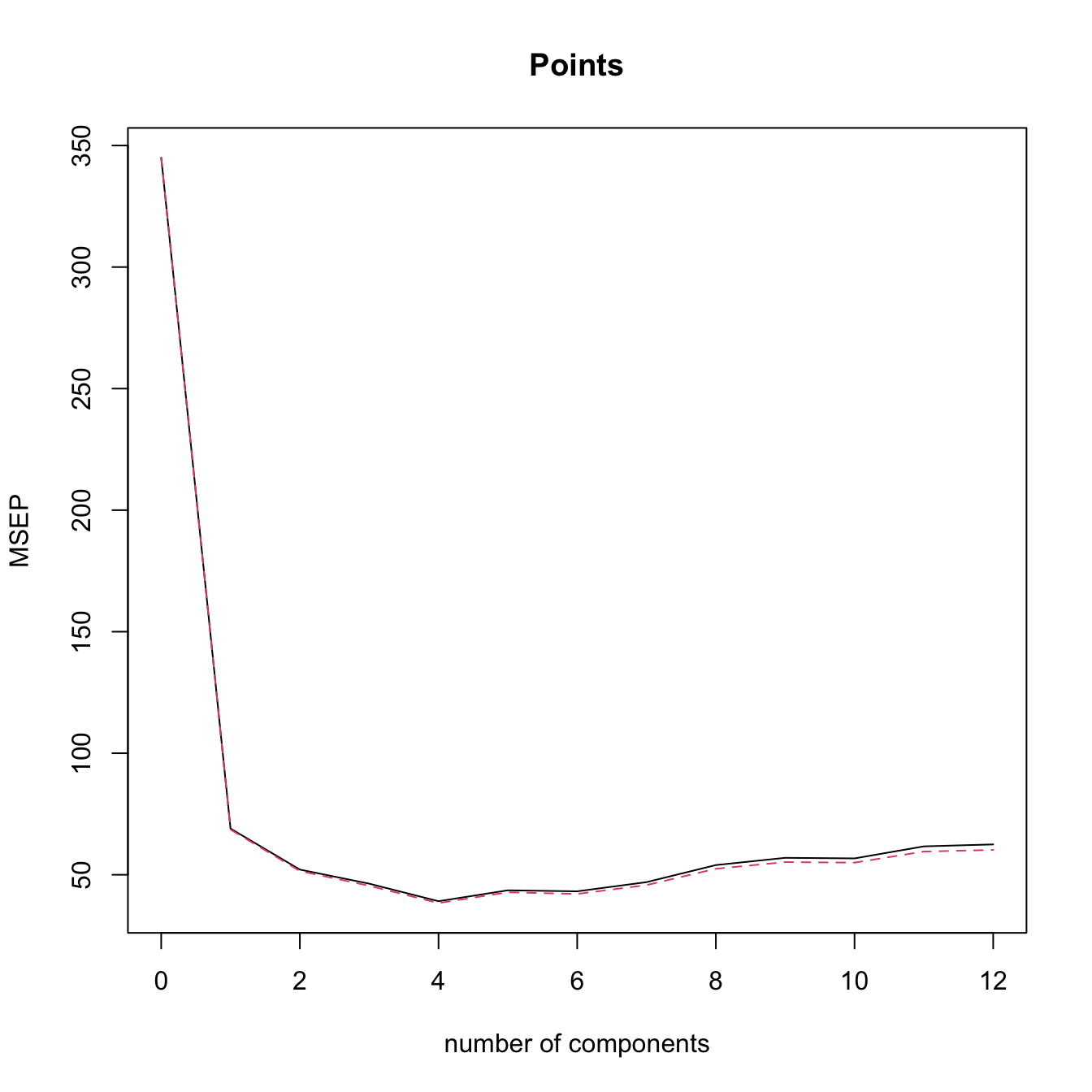

# Selecting the number of components to retain by 10-fold Cross-Validation
# (k = 10 is the default)
modPlsrCV10 <- plsr(Points ~ ., data = laligaRed2, scale = TRUE,
                    validation = "CV")
summary(modPlsrCV10)
## Data:    X dimension: 20 12 
##  Y dimension: 20 1
## Fit method: kernelpls
## Number of components considered: 12
## 
## VALIDATION: RMSEP
## Cross-validated using 10 random segments.
##        (Intercept)  1 comps  2 comps  3 comps  4 comps  5 comps  6 comps  7 comps  8 comps  9 comps  10 comps  11 comps
## CV           18.57    7.895    6.944    6.571    6.330    6.396    6.607    7.018    7.487    7.612     7.607     8.520
## adjCV        18.57    7.852    6.868    6.452    6.201    6.285    6.444    6.830    7.270    7.372     7.368     8.212
##        12 comps
## CV        8.014
## adjCV     7.714
## 
## TRAINING: % variance explained
##         1 comps  2 comps  3 comps  4 comps  5 comps  6 comps  7 comps  8 comps  9 comps  10 comps  11 comps  12 comps
## X         62.53    76.07    84.94    88.29    92.72    95.61    98.72    99.41    99.83    100.00    100.00    100.00
## Points    83.76    91.06    93.93    95.43    95.94    96.44    96.55    96.73    96.84     96.84     97.69     97.95
validationplot(modPlsrCV10, val.type = "MSEP")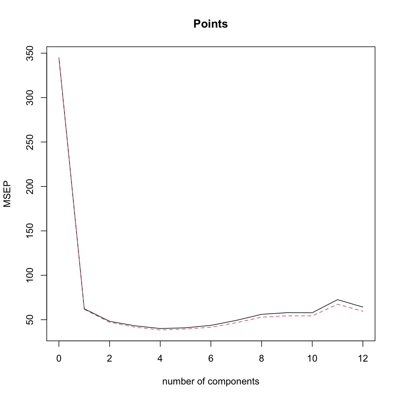

# l = 4 is close to the minimum CV

# Regress manually Points in the scores, in order to have an lm object
# Create a new dataset with the response + PLS components
laligaPLS <- data.frame("Points" = laliga$Points, cbind(modPlsr$scores))

# Regression on the first two PLS
modPlsr <- lm(Points ~ Comp.1 + Comp.2, data = laligaPLS)
summary(modPlsr) # Predictors clearly significant -- same R^2 as in modPlsr2
## 
## Call:
## lm(formula = Points ~ Comp.1 + Comp.2, data = laligaPLS)
## 
## Residuals:
##     Min      1Q  Median      3Q     Max 
## -9.3565 -3.6157  0.4508  2.3288 12.3116 
## 
## Coefficients:
##             Estimate Std. Error t value Pr(>|t|)    
## (Intercept)  52.4000     1.2799  40.941  < 2e-16 ***
## Comp.1        6.0933     0.4829  12.618 4.65e-10 ***
## Comp.2        4.3413     1.1662   3.723  0.00169 ** 
## ---
## Signif. codes:  0 '***' 0.001 '**' 0.01 '*' 0.05 '.' 0.1 ' ' 1
## 
## Residual standard error: 5.724 on 17 degrees of freedom
## Multiple R-squared:  0.9106, Adjusted R-squared:    0.9 
## F-statistic: 86.53 on 2 and 17 DF,  p-value: 1.225e-09
car::vif(modPlsr) # No problems at all
## Comp.1 Comp.2 
##      1      1

Exercise 3.15 Let’s perform PCR and PLSR in the iris dataset. Recall that this dataset contains a factor variable, which can not be treated directly by princomp but can be used in PCR/PLSR (it is transformed internally to two dummy variables). Do the following:

1. Compute the PCA of iris, excluding Species. What is the percentage of variability explained with two components?
2. Draw the biplot and look for interpretations of the principal components.
3. Plot the PCA scores in a car::scatterplotMatrix plot such that the scores are colored by the levels in Species (you can use the groups argument).
4. Compute the PCR of Petal.Width with \(\ell=2\) (exclude Species). Inspect by leave-one-out cross-validation the best selection of \(\ell.\)
5. Repeat the previous point with PLSR.
6. Plot the PLS scores of the data in a car::scatterplotMatrix plot such that the scores are colored by the levels in Species. Compare with the PCA scores. Is there any interesting interpretation? (A quick way of converting the scores to a matrix is with rbind.)

In theory, the dimensionality reduction of PLSR is more adequate for linear regression than that of PCR. However, in many practical situations PLSR and PCR tend to perform similarly, since the variance of the PLSR predictors \(P_1,\ldots,P_\ell\) is larger (due to the iterative linear-filtering procedure on which they are constructed) than the variance of the PCR predictors \(\Gamma_1,\ldots,\Gamma_\ell.\)

Inference for PLSR is more involved since, differently to what happens in PCR, the PLS directions are dependent on the response \(Y\). This directly breaks a core assumption made in Section 2.4: that the randomness of the regression model came only from the error terms and not from the predictors.

We conclude by illustrating the differences between PLSR and PCR with a small numerical example. For that, we consider two correlated predictors \[\begin{align} \begin{pmatrix}X_1\\X_2\end{pmatrix}\sim \mathcal{N}_2\left(\begin{pmatrix}0\\0\end{pmatrix},\begin{pmatrix}1&\rho\\\rho&1\end{pmatrix}\right), \quad -1\leq\rho\leq1,\tag{3.20} \end{align}\] and the linear model \[\begin{align} Y=\beta_1X_1+\beta_2X_2+\varepsilon,\quad \boldsymbol{\beta}=\begin{pmatrix}\cos(\theta)\\\sin(\theta)\end{pmatrix},\tag{3.21} \end{align}\] where \(\theta\in[0,2\pi)\) and \(\varepsilon\sim\mathcal{N}(0,1).\) Therefore:

• The correlation \(\rho\) controls the linear dependence between \(X_1\) and \(X_2\). This parameter is the only one that affects the two principal components \(\Gamma_1=a_{11}X_1+a_{21}X_2\) and \(\Gamma_2=a_{12}X_1+a_{22}X_2\) (recall (3.9)). The loadings \((\hat{a}_{11},\hat{a}_{21})^\top\) and \((\hat{a}_{12},\hat{a}_{22})^\top\) are the (sample) PC1 and PC2 directions.
• The angle \(\theta\) controls the direction of \(\boldsymbol{\beta},\) that is, the linear relation between \(Y\) and \((X_1,X_2)\). Consequently, \(\theta\) affects the PLS components \(P_1=b_{11}X_1+b_{21}X_2\) and \(P_2=b_{12}X_1+b_{22}X_2\) (recall (3.19), with adapted notation). The loadings \((\hat{b}_{11},\hat{b}_{21})^\top\) and \((\hat{b}_{12},\hat{b}_{22})^\top\) are the (sample) PLS1 and PLS2 directions.

The animation in Figure 3.35 contains samples from (3.20) colored according to their expected value under (3.21). It illustrates the following insights:

• PC directions are unaware of \(\boldsymbol{\beta};\) PLS directions are affected by \(\boldsymbol{\beta}.\)
• PC directions are always orthogonal; PLS directions are not.
• PLS1 aligns¹⁰² with \(\boldsymbol{\beta}\) when \(\rho = 0.\) This does not happen when \(\rho \neq 0\) (remember Figure 2.7).
• Under high correlation, the PLS and PC directions are very similar.
• Under low-moderate correlation, PLS1 better explains¹⁰³ \(\boldsymbol{\beta}\) than PC1.

Figure 3.35: Illustration of the differences and similarities between PCR and PLSR. The points are sampled from (3.20) and colored according to their expected value under (3.21): yellow for larger values; dark violet for smaller. The color gradient is thus controlled by the direction of \(\boldsymbol{\beta}\) (black arrow) and informs on the position of the plane \(y=\beta_1x_1+\beta_2x_2.\) The PC/PLS directions are described in the text. Application available here.

References

Box, G. E. P., and D. R. Cox. 1964. “An Analysis of Transformations.” Journal of the Royal Statistical Society, Series B (Methodological) 26 (2): 211–52. https://doi.org/10.1111/j.2517-6161.1964.tb00553.x.

Harrison, D., and D. L. Rubinfeld. 1978. “Hedonic Housing Prices and the Demand for Clean Air.” Journal of Environmental Economics and Management 5 (1): 81–102. https://doi.org/10.1016/0095-0696(78)90006-2.

Moore, G. E. 1965. “Cramming More Components onto Integrated Circuits.” Electronics 38 (8): 114–17. https://doi.org/10.1109/JPROC.1998.658762.

Peña, D. 2002. Regresión y Diseño de Experimentos. Madrid: Alianza Editorial. https://www.alianzaeditorial.es/libro/manuales/regresion-y-diseno-de-experimentos-daniel-pena-9788420693897/.

Schwarz, G. 1978. “Estimating the Dimension of a Model.” The Annals of Statistics 6 (2): 461–64. https://doi.org/10.1214/aos/1176344136.

Shao, J. 1993. “Linear Model Selection by Cross-Validation.” Journal of the American Statistical Association 88 (422): 486–94. https://doi.org/10.2307/2290328.

Yeo, I.-K., and R. A. Johnson. 2000. “A New Family of Power Transformations to Improve Normality or Symmetry.” Biometrika 87 (4): 954–59. https://doi.org/10.1093/biomet/87.4.954.

---

51. A hedonic model is a model that decomposes the price of an item into separate components that determine its price. For example, a hedonic model for the price of a house may decompose its price into the house characteristics, the kind of neighborhood, and the location.↩︎

52. But be aware of the changes in units for medv, black, lstat, and nox.↩︎

53. Applying its formula, we would obtain \(\hat\sigma^2=0/0\) and so \(\hat\sigma^2\) will not be defined.↩︎

54. Of course, with the same responses.↩︎

55. Recall that \(\log(n)>2\) if \(n\geq8.\)↩︎

56. Also, because the BIC is consistent, see Section 3.2.2.↩︎

57. Since we have to take \(p\) binary decisions on whether to include or not each of the \(p\) predictors.↩︎

58. The function always prints ‘AIC’, even if ‘BIC’ is employed.↩︎

59. Note the - before FrancePop. Note also the convenient sorting of the BICs in an increasing form, so that the next best action always corresponds to the first row.↩︎

60. If possible!↩︎

61. The specifics of this result for the linear model are given in Schwarz (1978).↩︎

62. Cross-validation and its different variants are formally addressed at the end of Section 3.6.2.↩︎

63. To account for the \(J-1\) possible departures from a reference level.↩︎

64. In particular, Taylor’s theorem allows to approximate a sufficiently regular function \(m\) by a polynomial, which is identifiable with a multiple linear model as seen in Section 3.4.2. This idea, applied locally, is elaborated in Section 6.2.2.↩︎

65. The consideration of more than one predictor is conceptually straightforward, yet notationally more cumbersome.↩︎

66. Precisely, the type of orthogonal polynomials considered are a data-driven shifting and rescaling of the Legendre polynomials in \((-1,1).\) The Legendre polynomials \(p_j\) and \(p_\ell\) in \((-1,1)\) satisfy that \(\int_{-1}^1 p_j(x)p_\ell(x)\,\mathrm{d}x=\frac{2}{2j+1}\delta_{j\ell},\) where \(\delta_{j\ell}\) is the Kronecker’s delta. The first five Legendre polynomials in \((-1,1)\) are, respectively: \(p_1(x)=x,\) \(p_2(x)=\frac{1}{2}(3x^2-1),\) \(p_3(x)=\frac{1}{2}(5x^3-3x),\) \(p_4(x)=\frac{1}{8}(35x^4-30x^2+3),\) and \(p_5(x)=\frac{1}{8}(63x^5-70x^3+15x).\) Also, \(p_0(x)=1.\) The recursive formula \(p_{k+1}(x)=(k+1)^{-1}\big[(2k+1)xp_k(x)-kp_{k-1}(x)\big]\) allows to obtain the \((k+1)\)-th order Legendre polynomial from the previous two ones. Notice that from \(k\geq 3,\) \(p_k(x)\) involves more monomials than just \(x^k,\) precisely all the monomials with a lower order and with the same parity. This may complicate the interpretation of a coefficient related to \(p_k(X)\) for \(k\geq3,\) as it is not directly associated to a \(k\)-th order effect of \(X.\)↩︎

67. This is due to how the second matrix of (3.5) is computed: by means of a \(QR\) decomposition associated to the first matrix. The decomposition yields a data matrix formed by polynomials that are not exactly the Legendre polynomials but a data-driven shifting and rescaling of them.↩︎

68. Of course, the roles of \(X_1\) and \(X_2\) can be interchanged in this interpretation.↩︎

69. If \(p=1,\) then it is possible to inspect the scatterplot of the \(\{(X_{i1},Y_i)\}_{i=1}^n\) in order to determine whether linearity is plausible. But the usefulness of this graphical check quickly decays with the dimension \(p,\) as \(p\) scatterplots need to be investigated. That is precisely the key point for relying in the residuals vs. fitted values plot.↩︎

70. Assume that \(f(Y)=\beta_0+\beta_1X+\varepsilon,\) with \(f\) nonlinear and invertible. Clearly, \(W=f(Y)\) satisfies \(W=\beta_0+\beta_1X+\varepsilon,\) and we can estimate \(\mathbb{E}[W \mid X=x]\) with \(\hat{w}=\hat{\beta}_0+\hat{\beta}_1x\) unbiasedly, i.e., \(\mathbb{E}[\hat{w} \mid X_1,\ldots,X_n]=\mathbb{E}[W \mid X=x].\) Define \(\hat{y}_f:=f^{-1}(\hat{w}).\) Because of the delta method (see next footnote), \(\mathbb{E}[\hat{y}_f \mid X_1,\ldots,X_n]\) is asymptotically equal to \(f^{-1}(\mathbb{E}[W \mid X=x]).\) However, \(f^{-1}(\mathbb{E}[W \mid X=x])\neq (\mathbb{E}[f^{-1}(W) \mid X=x])=\mathbb{E}[Y \mid X=x],\) so \(\hat{y}_f\) is a biased estimator of \(\mathbb{E}[Y \mid X=x].\) Indeed, if \(f\) is strictly convex (e.g., \(f=\log\)), then \(f^{-1}\) is strictly concave, and Jensen’s inequality guarantees that \(f^{-1}(\mathbb{E}[W \mid X=x])\geq \mathbb{E}[f^{-1}(W) \mid X=x],\) that is, \(\hat{y}_f\) underestimates \(\mathbb{E}[Y \mid X=x].\)↩︎

71. Delta method. Let \(\hat{\theta}\) be an estimator of \(\theta\) such that \(\sqrt{n}(\hat{\theta}-\theta)\) is asymptotically a \(\mathcal{N}(0,\sigma^2)\) when \(n\to\infty.\) If \(g\) is a real-valued function such that \(g'(\theta)\neq0\) exists, then \(\sqrt{n}(g(\hat{\theta})-g(\theta))\) is asymptotically a \(\mathcal{N}(0,\sigma^2(g'(\theta))^2).\)↩︎

72. Given that removing the bias introduced by considering \(\hat{Y}_f=f^{-1}(\hat{W})\) is challenging.↩︎

73. Recall that \(\hat\beta_j=\mathbf{e}_j^ op(\mathbf{X}^ op\mathbf{X})^{-1}\mathbf{X}^ op\mathbf{Y}=:\sum_{i=1}^nw_{ij}Y_i,\) where \(\mathbf{e}_j\) is the canonical vector of \(\mathbb{R}^{p+1}\) with \(1\) in the \(j\)-th position and \(0\) elsewhere. Therefore, \(\hat\beta_j\) is a weighted sum of the random variables \(Y_1,\ldots,Y_n\) (recall that we assume that \(\mathbf{X}\) is given and therefore is deterministic). Even if \(Y_1,\ldots,Y_n\) are not normal, the central limit theorem entails that \(\sqrt{n}(\hat\beta_j-\beta_j)\) is asymptotically normally distributed when \(n\to\infty,\) provided that linearity holds.↩︎

74. Distributions that are not heavy tailed, not heavily multimodal, and not heavily skewed.↩︎

75. For \(X\sim F,\) the \(p\)-th quantile \(x_p=F^{-1}(p)\) of \(X\) is estimated through the sample quantile \(\hat{x}_p:=F_n^{(-1)}(p),\) where \(F_n(x)=\frac{1}{n}\sum_{i=1}^n1_{\{X_i\leq x\}}\) is the empirical cdf of \(X_1,\ldots,X_n\) and \(F_n^{(-1)}\) is the generalized inverse function of \(F_n.\) If \(X\sim f\) is continuous, then \(\sqrt{n}(\hat{x}_p-x_p)\) is asymptotically a \(\mathcal{N}\left(0,\frac{p(1-p)}{f(x_p)^2}\right).\) Therefore, the variance of \(\hat x_p\) grows if \(p\to0\) or \(p\to1,\) hence more variability is expected on the extremes of the QQ-plot (see Figure 3.20).↩︎

76. This is the Kolmogorov–Smirnov test shown in Section A but adapted to testing the normality of the data with unknown mean and variance. More precisely, the test tests the composite null hypothesis \(H_0:F=\Phi(\cdot;\mu,\sigma^2)\) with \(\mu\) and \(\sigma^2\) unknown. Note that this is different from the simple null hypothesis \(H_0:F=F_0\) of the Kolmogorov–Smirnov test in which \(F_0\) is completely specified. Further tests of normality can be derived by adapting other tests for the simple null hypothesis \(H_0:F=F_0,\) such as the Cramér–von Mises and the Anderson–Darling tests, and these are implemented in the functions nortest::cvm.test and nortest::ad.test.↩︎

77. Precisely, if \(\lambda<1,\) positive skewness (or skewness to the right) is palliated (large values of \(Y\) shrink, small values grow), whereas if \(\lambda>1\) negative skewness (or skewness to the left) is corrected (large values of \(Y\) grow, small values shrink).↩︎

78. Maximum likelihood for a \(\mathcal{N}(\mu,\sigma^2)\) and potentially using the linear model structure if we are performing the transformation to achieve normality in errors of the linear model. Recall that optimally transforming \(Y\) such that \(Y\) is normal-like or \(Y \mid (X_1,\ldots,X_p)\) is normal-like (the assumption in the linear model) are very different goals!↩︎

79. And therefore more informative on the linear dependence of the predictors than the correlations of \(X_j\) with each of the remaining predictors.↩︎

80. This is the expected value for the leverage statistic \(h_i\) if the linear model holds. However, the distribution of \(h_i\) depends on the joint distribution of the predictors \((X_1,\ldots,X_p).\)↩︎

81. That is, \(\mathbb{E}[X_j]=0,\) \(j=1,\ldots,p.\) This is important since PCA is sensitive to the centering of the data.↩︎

82. Recall that the covariance matrix is a real, symmetric, semi-positive definite matrix.↩︎

83. Therefore, \(\mathbf{A}^{-1}=\mathbf{A}^\top.\)↩︎

84. Since the variance-covariance matrix \(\mathbb{V}\mathrm{ar}[\boldsymbol{\Gamma}]\) is diagonal.↩︎

85. Up to now, the exposition has been focused exclusively on the population case.↩︎

86. Some care is needed here. The matrix \(\mathbf{S}\) is obtained from linear combinations of the \(n\) vectors \(\mathbf{X}_1-\bar{\mathbf{X}},\ldots,\mathbf{X}_n-\bar{\mathbf{X}}.\) Recall that these \(n\) vectors are not linearly independent, as they are guaranteed to add \(\mathbf{0},\) \(\sum_{i=1}^n[\mathbf{X}_i-\bar{\mathbf{X}}]=\mathbf{0},\) so it is possible to express one perfectly on the rest. That implies that the \(p\times p\) matrix \(\mathbf{S}\) has rank smaller or equal to \(n-1.\) If \(p\leq n-1,\) then the matrix has full rank \(p\) and it is invertible (excluding degenerate cases in which the \(p\) variables are collinear). But if \(p\geq n,\) then \(\mathbf{S}\) is singular and, as a consequence, \(\lambda_j=0\) for \(j\geq n.\) This implies that the principal components for those eigenvalues cannot be determined univocally.↩︎

87. Therefore, a sample of lengths measured in centimeters will have a variance \(10^4\) times larger than the same sample measured in meters – yet it is the same information!↩︎

88. The biplot is implemented in R by biplot.princomp (or by biplot applied to a princomp object). This function applies an internal scaling of the scores and variables to improve the visualization (see ?biplot.princomp), which can be disabled with the argument scale = 0.↩︎

89. For the sample version, replace the variable \(X_j\) by its sample \(X_{1j},\ldots,X_{nj},\) the loadings \(a_{ji}\) by their estimates \(\hat a_{ji},\) and the principal component \(\Gamma_j\) by the scores \(\{\hat{\Gamma}_{ij}\}_{i=1}^n.\)↩︎

90. Observe that both \(X_j=a_{j1}\Gamma_{1} + a_{j2}\Gamma_{2} + \cdots + a_{jp}\Gamma_{p}\) and \(\Gamma_j=a_{1j}X_{1} + a_{2j}X_{2} + \cdots + a_{pj}X_{p},\) \(j=1,\ldots,p,\) hold simultaneously due to the orthogonality of \(\mathbf{A}.\)↩︎

91. The first two principal components of the dataset explain the \(78\%\) of the variability of the data. Hence, the insights obtained from the biplot should be regarded as “\(78\%\)-accurate”.↩︎

92. This is certainly not always true, but it is often the case. See Figure 3.35.↩︎

93. For the sake of simplicity, we consider only the first \(\ell\) principal components, but obviously other combinations of \(\ell\) principal components are possible.↩︎

94. Since we know by (3.11) that \(\boldsymbol{\Gamma}=\mathbf{A}^\top(\mathbf{X}-\boldsymbol{\mu}),\) where \(\mathbf{A}\) is the \(p\times p\) matrix of loadings.↩︎

95. For example, thanks to \(\hat{\boldsymbol{\gamma}}\) we know that the estimated conditional response of \(Y\) precisely increases \(\hat{\gamma}_j\) units for a marginal unit increment in \(X_j.\)↩︎

96. If \(\ell=p,\) then PCR is equivalent to least squares estimation.↩︎

97. Alternatively, the “in Prediction” part of the latter terms is dropped and they are just referred to as the MSE and RMSE.↩︎

98. Compare (3.19) with (3.9).↩︎

99. Recall (2.3) for the sample version.↩︎

100. They play the role of \(X_1,\ldots,X_p\) in the computation of \(P_1\) and can be regarded as \(X_1,\ldots,X_p\) after filtering the linear information explained by \(P_1.\)↩︎

101. Of course, in practice, the computations need to be done in terms of the sample versions of the presented population versions.↩︎

102. Recall that we do not care about whether the directions of PLS1 and \(\boldsymbol{\beta}\) are close, but rather if the axes spanned by PLS1 and \(\boldsymbol{\beta}\) are close. The signs of \(\boldsymbol{\beta}\) are learned during the model fitting!↩︎

103. In the sense that the absolute value of the projection of \(\boldsymbol{\beta}\) along \((\hat{b}_{11},\hat{b}_{21})^\top,\) \(|(\hat{b}_{11},\hat{b}_{21})\boldsymbol{\beta}|,\) is usually larger than that along \((\hat{a}_{11},\hat{a}_{21})^\top.\)↩︎