4 Linear models III: shrinkage, multivariate response, and big data
We explore in this chapter several extensions of the linear model for certain non-classical settings such as: high-dimensional data (\(p\gg n\)) that requires shrinkage methods, big data (large \(n\)) that demands thoughtful computations, and the multivariate response situation in which the interest lies in explaining a vector of responses \(\mathbf{Y}=(Y_1,\ldots,Y_q).\)
4.1 Shrinkage
As we saw in Section 2.4.1, the least squares estimates \(\hat{\boldsymbol{\beta}}\) of the linear model
\[\begin{align*} Y = \beta_0 + \beta_1 X_1 + \cdots + \beta_p X_p + \varepsilon \end{align*}\]
were the minimizers of the residual sum of squares
\[\begin{align*} \text{RSS}(\boldsymbol{\beta})=\sum_{i=1}^n(Y_i-\beta_0-\beta_1X_{i1}-\cdots-\beta_pX_{ip})^2. \end{align*}\]
Under the validity of the assumptions of Section 2.3, in Section 2.4 we saw that
\[\begin{align*} \hat{\boldsymbol{\beta}}\sim\mathcal{N}_{p+1}\left(\boldsymbol{\beta},\sigma^2(\mathbb{X}^\top\mathbb{X})^{-1}\right). \end{align*}\]
A particular consequence of this result is that \(\hat{\boldsymbol{\beta}}\) is unbiased in estimating \(\boldsymbol{\beta},\) that is, \(\hat{\boldsymbol{\beta}}\) does not make any systematic error in estimating \(\boldsymbol{\beta}.\) However, bias is only one part of the quality of an estimate: variance is also important. Indeed, the bias-variance trade-off106 arises from the bias-variance decomposition of the Mean Squared Error (MSE) of an estimate. For example, for the estimate \(\hat\beta_j\) of \(\beta_j,\) we have
\[\begin{align} \mathrm{MSE}[\hat\beta_j]:=\mathbb{E}[(\hat\beta_j-\beta_j)^2]=\underbrace{(\mathbb{E}[\hat\beta_j]-\beta_j)^2}_{\mathrm{Bias}^2}+\underbrace{\mathbb{V}\mathrm{ar}[\hat\beta_j]}_{\mathrm{Variance}}.\tag{4.1} \end{align}\]
In view of (4.1), one might be tempted to minimize the MSE sequentially: first zero out the bias and then minimize the variance subject to that zero-bias constraint. That happened to be the strategy followed by the least squares estimates \(\hat{\boldsymbol{\beta}}\). This is a very natural strategy, and it has been very influential in the development of statistics.107 However, it is important to realize that this strategy is suboptimal in terms of the MSE in most cases, since tolerating some bias can yield a much smaller variance — and hence a smaller MSE. As an example, consider minimizing \(f(x,y)=g(x,y)+h(x,y),\) for \(g,h\geq 0,\) where \(g\) plays the role of the squared bias and \(h\) that of the variance. Figure 4.1 shows that \(\min_{(x,y)\in\mathbb{R}^2} f(x,y) < \min_{(x,y)\in\mathbb{R}^2:\,g(x,y)=0} h(x,y),\) so joint minimization beats the sequential one.
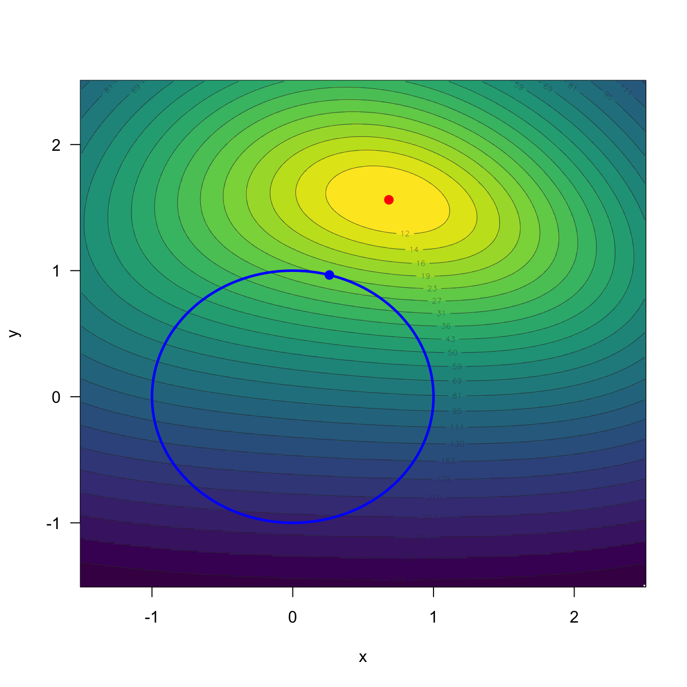
Figure 4.1: Illustration of the suboptimality of the sequential “first bias, then variance” minimization strategy in a toy optimization problem. The contour plot shows \(f(x,y)=g(x,y)+h(x,y)\) with \(g(x,y)=(x^2+y^2-1)^2\) and \(h(x,y)=|x-2|^3+(y-3)^4,\) where \(g\) plays the role of the squared bias and \(h\) that of the variance. The blue circle is the region \(\{(x,y)\in\mathbb{R}^2:g(x,y)=0\}\) where the bias-analog vanishes; the blue point is the minimizer of \(h\) over that region. The red point is the joint minimizer of \(f.\) Even though the blue point achieves \(g=0,\) the red point attains a strictly smaller value of \(f\).
Building on the previous discussion, shrinkage methods pursue the following idea:
Add an amount of smart bias to \(\hat{\boldsymbol{\beta}}\) in order to reduce its variance, in such a way that we obtain simpler interpretations from the biased version of \(\hat{\boldsymbol{\beta}}.\)
This idea is implemented by enforcing sparsity, that is, by biasing the estimates of \(\boldsymbol{\beta}\) towards being non-null only for the most important predictors. The two main methods covered in this section, ridge regression and lasso (least absolute shrinkage and selection operator), use this idea in a different way. However, it is important to realize that both methods do consider the standard linear model; what they do differently is the way of estimating \(\boldsymbol{\beta}\).
The way they enforce sparsity in the estimates is by minimizing the RSS plus a penalty term that favors sparsity on the estimated coefficients. For example, the ridge regression enforces a quadratic penalty to the candidate slope coefficients \(\boldsymbol\beta_{-1}=(\beta_1,\ldots,\beta_p)^\top\) and seeks to minimize108
\[\begin{align} \text{RSS}(\boldsymbol{\beta})+\lambda\sum_{j=1}^p \beta_j^2=\text{RSS}(\boldsymbol{\beta})+\lambda\|\boldsymbol\beta_{-1}\|_2^2,\tag{4.2} \end{align}\]
where \(\lambda\geq 0\) is the penalty parameter. On the other hand, the lasso considers an absolute penalty:
\[\begin{align} \text{RSS}(\boldsymbol{\beta})+\lambda\sum_{j=1}^p |\beta_j|=\text{RSS}(\boldsymbol{\beta})+\lambda\|\boldsymbol\beta_{-1}\|_1.\tag{4.3} \end{align}\]
A visualization of the absolute and squared norms is given in Figure 4.2 (in \(\mathbb{R}^2\)) and Figure 4.3 (in \(\mathbb{R}^3\)).
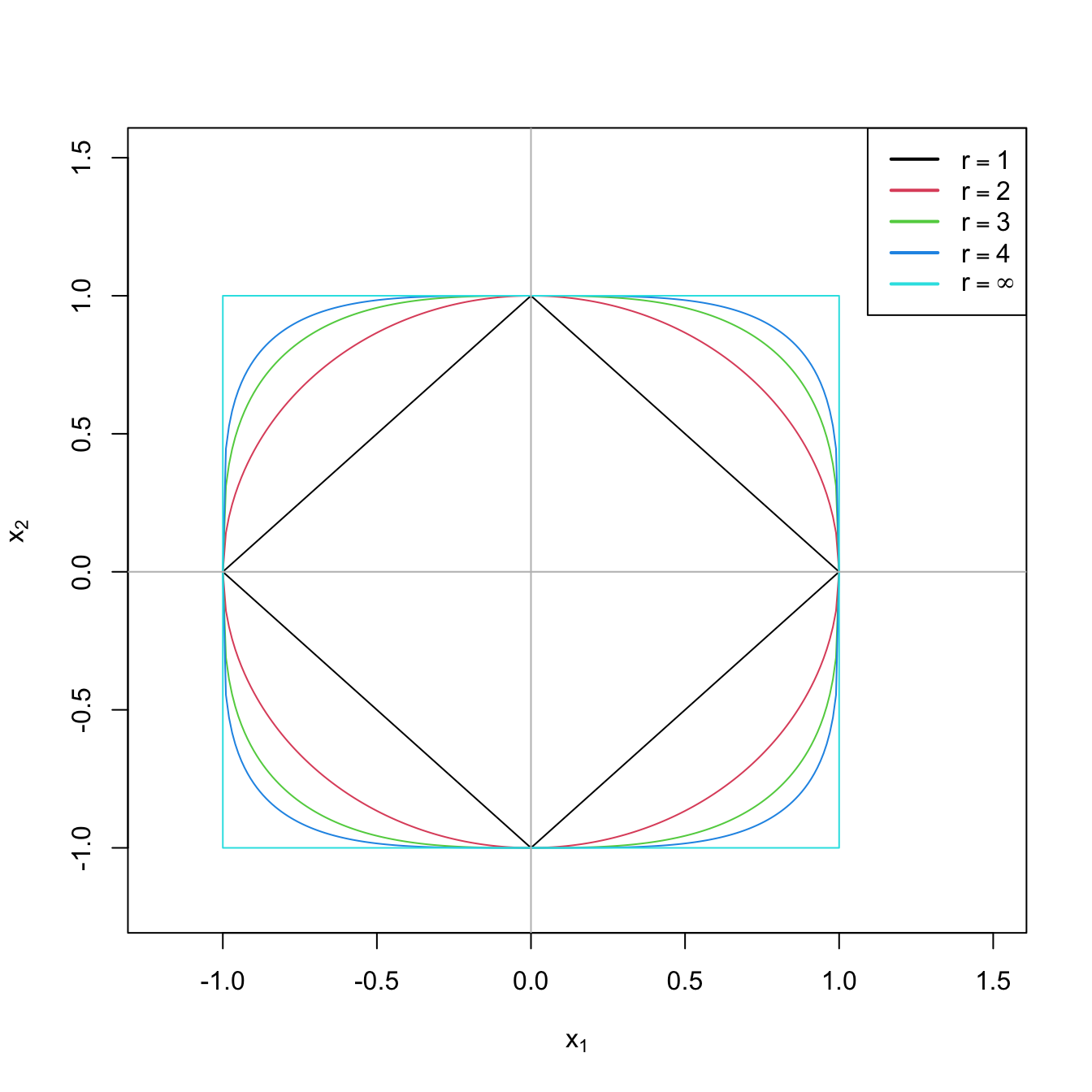
Figure 4.2: The “unit circle” \(\|(x_1,x_2)\|_r=1\) for \(r=1,2,4,\infty\).
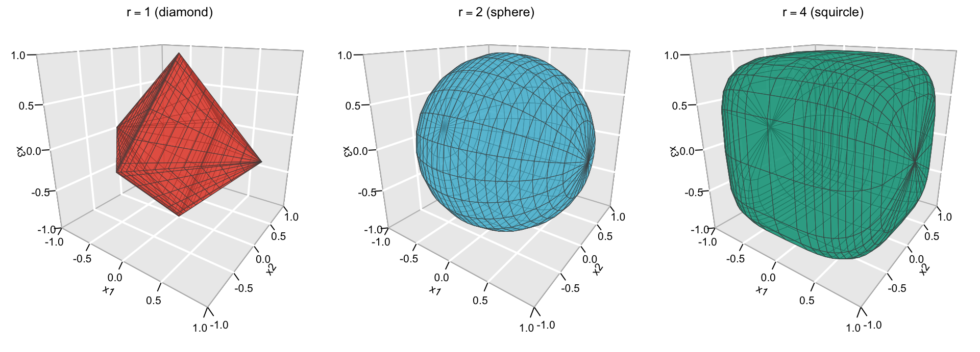
Figure 4.3: The “unit sphere” \(\|(x_1,x_2,x_3)\|_r=1\) for \(r=1\) (diamond, left), \(r=2\) (sphere, middle), and \(r=4\) (squircle, right).
Among other possible joint representations for (4.2) and (4.3),109 the one based on the elastic nets is particularly convenient, as it aims to combine the strengths of both methods in a computationally tractable way and is the one employed in the reference package glmnet. Considering a proportion \(0\leq\alpha\leq 1,\) the elastic net is defined as
\[\begin{align} \text{RSS}(\boldsymbol{\beta})+\lambda(\alpha\|\boldsymbol\beta_{-1}\|_1+(1-\alpha)\|\boldsymbol\beta_{-1}\|_2^2).\tag{4.4} \end{align}\]
Clearly, ridge regression corresponds to \(\alpha=0\) (quadratic penalty) and lasso to \(\alpha=1\) (absolute penalty). Obviously, if \(\lambda=0,\) we are back to the least squares problem and theory. The optimization of (4.4) gives
\[\begin{align} \hat{\boldsymbol{\beta}}_{\lambda,\alpha}:=\arg\min_{\boldsymbol{\beta}\in\mathbb{R}^{p+1}}\left\{ \text{RSS}(\boldsymbol{\beta})+\lambda\sum_{j=1}^p (\alpha|\beta_j|+(1-\alpha)|\beta_j|^2)\right\},\tag{4.5} \end{align}\]
which is the penalized estimation of \(\boldsymbol{\beta}.\) Note that the sparsity is enforced in the slopes, not in the intercept, since this depends on the mean of \(Y.\) Note also that the optimization problem is convex110 and therefore it is guaranteed the existence and uniqueness of a minimum. However, in general,111 there are no explicit formulas for \(\hat{\boldsymbol{\beta}}_{\lambda,\alpha}\) and the optimization problem needs to be solved numerically. Finally, \(\lambda\) is a tuning parameter that will need to be chosen suitably and that we will discuss later.112 What it is important now is to recall that the predictors need to be standardized, or otherwise its scale will distort the optimization of (4.4).
An equivalent way of viewing (4.5) that helps in visualizing the differences between the ridge and lasso regressions is that they try to solve the equivalent optimization problem113 of (4.5):
\[\begin{align} \hat{\boldsymbol{\beta}}_{s_\lambda,\alpha}:=\arg\min_{\boldsymbol{\beta}\in\mathbb{R}^{p+1}:\sum_{j=1}^p (\alpha|\beta_j|+(1-\alpha)|\beta_j|^2)\leq s_\lambda} \text{RSS}(\boldsymbol{\beta}),\tag{4.6} \end{align}\]
where \(s_\lambda\) is certain scalar that does not depend on \(\boldsymbol{\beta}.\)
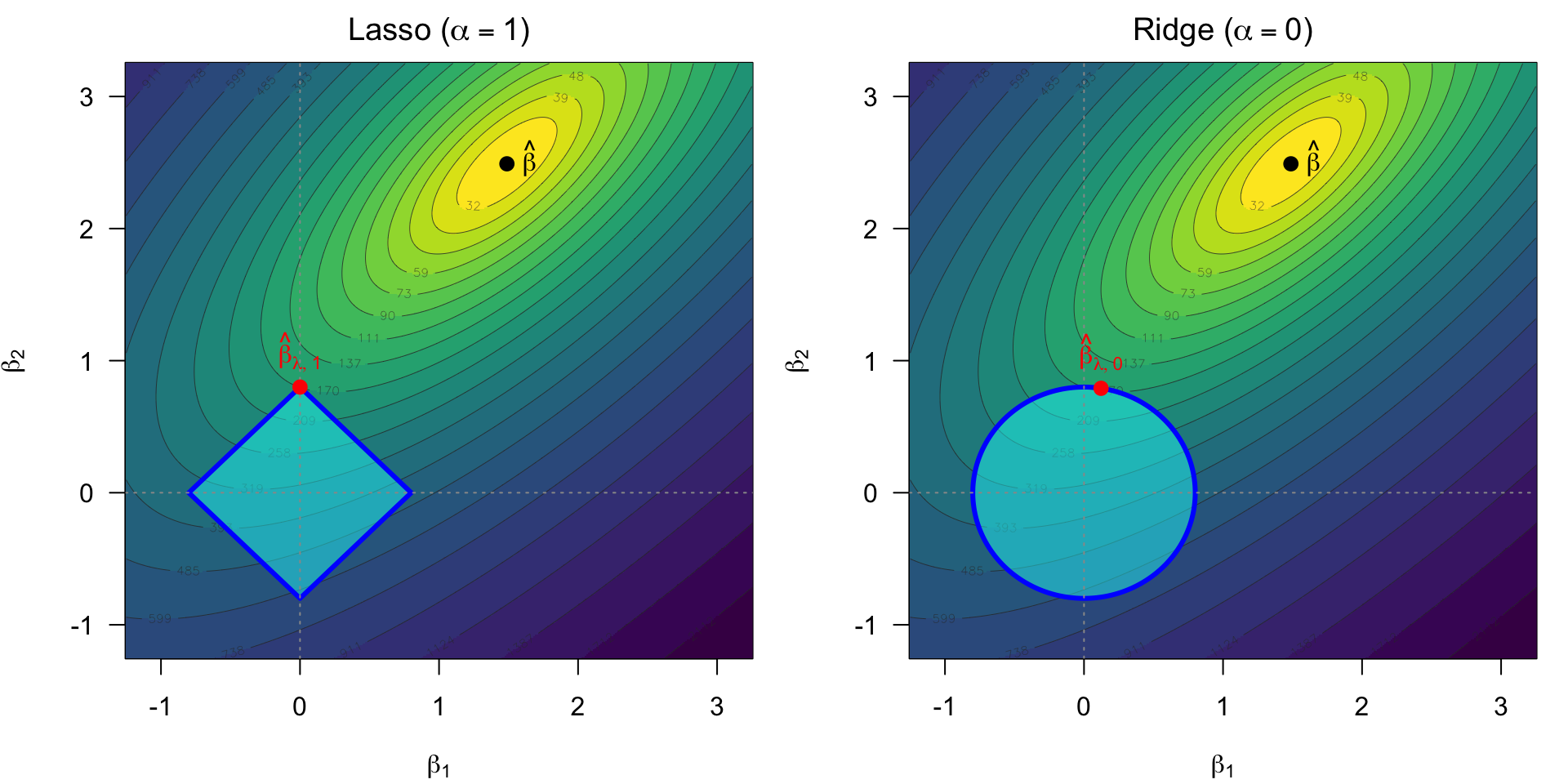
Figure 4.4: Comparison of ridge and lasso solutions from the optimization problem (4.6) with \(p=2.\) The background contours show the \(\mathrm{RSS}(\beta_1,\beta_2)\) surface (yellow marks its minimum, the least-squares estimate \(\hat{\boldsymbol\beta}\)); \(\beta_0=0\) is assumed. The diamond (\(\alpha=1\)) and circular (\(\alpha=0\)) cyan regions show the feasibility regions \(\sum_{j=1}^p (\alpha|\beta_j|+(1-\alpha)|\beta_j|^2)\leq s_\lambda\) for the optimization problem (4.6). The constrained minimizers are \(\hat{\boldsymbol{\beta}}_{\lambda,1}\) (lasso) and \(\hat{\boldsymbol{\beta}}_{\lambda,0}\) (ridge). The sharpness of the diamond makes the lasso attain solutions with coefficients exactly equal to zero, as happens here with \(\hat\beta_{\lambda,1,1}=0.\) Figure inspired from James et al. (2013).
The glmnet package is the reference implementation of shrinkage estimators based on elastic nets. In order to illustrate how to apply the ridge and lasso regression in practice, we will work with the ISLR::Hitters dataset. This dataset contains statistics and salaries from baseball players from the 1986 and 1987 seasons. The objective will be to predict the Salary from the remaining predictors.
# Load data -- baseball players statistics
data(Hitters, package = "ISLR")

# Discard NA's
Hitters <- na.omit(Hitters)

# The glmnet function works with the design matrix of predictors (without
# the ones). This can be obtained easily through model.matrix()
x <- model.matrix(Salary ~ ., data = Hitters)[, -1]
# [, -1] to remove the column of 1's associated with the intercept, since the
# intercept will be added by default in glmnet::glmnet and if we do not exclude
# it here we will end with two intercepts in the fit, one of them being NA.

# Interestingly, note that in Hitters there are two-level factors and these
# are automatically transformed into dummy variables in x -- the main advantage
# of model.matrix
head(Hitters[, 14:20])
##                   League Division PutOuts Assists Errors Salary NewLeague
## -Alan Ashby            N        W     632      43     10  475.0         N
## -Alvin Davis           A        W     880      82     14  480.0         A
## -Andre Dawson          N        E     200      11      3  500.0         N
## -Andres Galarraga      N        E     805      40      4   91.5         N
## -Alfredo Griffin       A        W     282     421     25  750.0         A
## -Al Newman             N        E      76     127      7   70.0         A
head(x[, 14:19])
##                   LeagueN DivisionW PutOuts Assists Errors NewLeagueN
## -Alan Ashby             1         1     632      43     10          1
## -Alvin Davis            0         1     880      82     14          0
## -Andre Dawson           1         0     200      11      3          1
## -Andres Galarraga       1         0     805      40      4          1
## -Alfredo Griffin        0         1     282     421     25          0
## -Al Newman              1         0      76     127      7          0

# We also need the vector of responses
y <- Hitters$Salary
model.matrix removes by default the observations with any NAs, returning only the complete cases. This may be undesirable in certain circumstances. If NAs are to be preserved, an option is to use na.action = "na.pass" but with the function model.matrix.lm (not model.matrix, as it ignores the argument!).
model.matrix(y ~ 0 + ., data = data) creates a model matrix with no intercept, but with undesirable side effects. In particular, if there are factors in data, the first factor will receive as many dummies as levels it has, and the rest of the factors will receive one dummy less than the number of levels (as customary). This will be problematic: we are adding multicollinearity and uneven treatment of the factors in the model.
The next code illustrates the previous warnings.
# Data with NA in the first observation and factors with two levels
data_na <- data.frame("x1" = rnorm(3), "x2" = factor(c("A", "B", "A")),
                      "x3" = factor(c("F", "F", "M")), "y" = rnorm(3))
data_na$x1[1] <- NA

# The first observation disappears!
model.matrix(y ~ ., data = data_na)
##   (Intercept)         x1 x2B x3M
## 2           1  0.5136652   1   0
## 3           1 -0.6558154   0   1
## attr(,"assign")
## [1] 0 1 2 3
## attr(,"contrasts")
## attr(,"contrasts")$x2
## [1] "contr.treatment"
##
## attr(,"contrasts")$x3
## [1] "contr.treatment"

# Still removes NA's
model.matrix(y ~ ., data = data_na, na.action = "na.pass")
##   (Intercept)         x1 x2B x3M
## 2           1  0.5136652   1   0
## 3           1 -0.6558154   0   1
## attr(,"assign")
## [1] 0 1 2 3
## attr(,"contrasts")
## attr(,"contrasts")$x2
## [1] "contr.treatment"
##
## attr(,"contrasts")$x3
## [1] "contr.treatment"

# Does not remove NA's
model.matrix.lm(y ~ ., data = data_na, na.action = "na.pass")
##   (Intercept)         x1 x2B x3M
## 1           1         NA   0   0
## 2           1  0.5136652   1   0
## 3           1 -0.6558154   0   1
## attr(,"assign")
## [1] 0 1 2 3
## attr(,"contrasts")
## attr(,"contrasts")$x2
## [1] "contr.treatment"
##
## attr(,"contrasts")$x3
## [1] "contr.treatment"

# If y ~ 0 + ., the first factor gets two dummies instead of one!
model.matrix(y ~ 0 + ., data = data_na)
##           x1 x2A x2B x3M
## 2  0.5136652   0   1   0
## 3 -0.6558154   1   0   1
## attr(,"assign")
## [1] 1 2 2 3
## attr(,"contrasts")
## attr(,"contrasts")$x2
## [1] "contr.treatment"
##
## attr(,"contrasts")$x3
## [1] "contr.treatment"
4.1.1 Ridge regression
We describe next how to do the fitting, tuning parameter selection, prediction, and the computation of the analytical form for the ridge regression. The first three topics are very similar for the lasso or for other elastic net fits (i.e., without \(\alpha=0\)).
4.1.1.1 Fitting
# Call to the main function -- use alpha = 0 for ridge regression
library(glmnet)
ridge_mod <- glmnet(x = x, y = y, alpha = 0)
# By default, it computes the ridge solution over a set of lambdas
# automatically chosen. It also standardizes the variables by default to make
# the model fitting, since the penalization is scale-sensitive. Importantly,
# the coefficients are returned on the original scale of the predictors

# Plot of the solution path -- gives the value of the coefficients for different
# measures in xvar (penalization imposed to the model or fitness)
plot(ridge_mod, xvar = "norm", label = TRUE)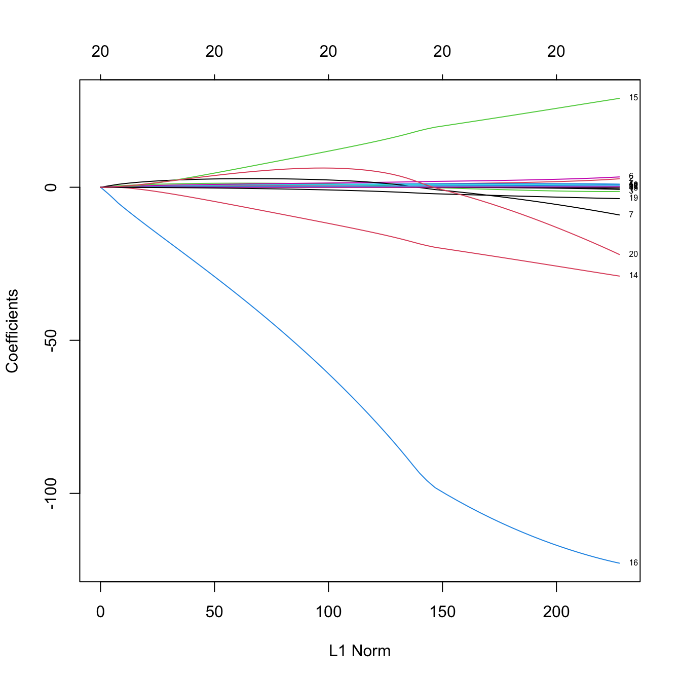
# xvar = "norm" is the default: L1 norm of the coefficients sum_j abs(beta_j)

# Versus lambda
plot(ridge_mod, label = TRUE, xvar = "lambda")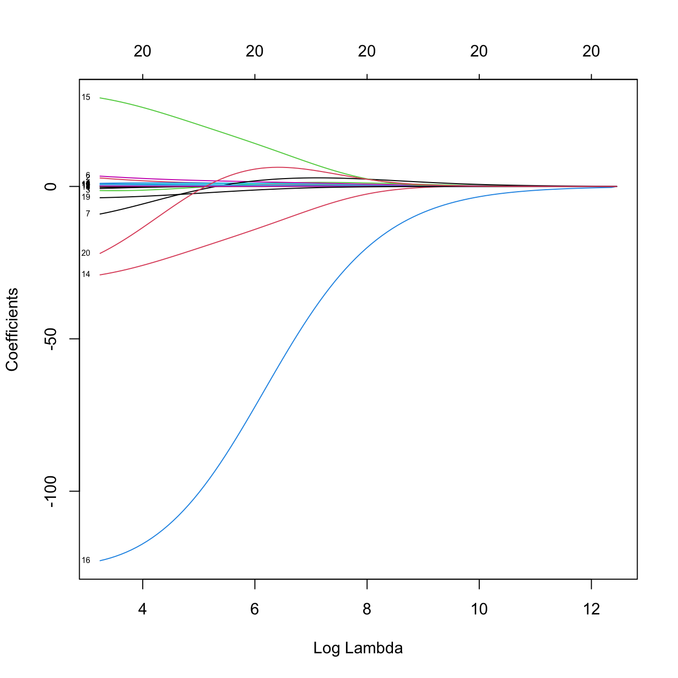
# Versus the percentage of deviance explained -- this is a generalization of the
# R^2 for generalized linear models. Since we have a linear model, this is the
# same as the R^2
plot(ridge_mod, label = TRUE, xvar = "dev")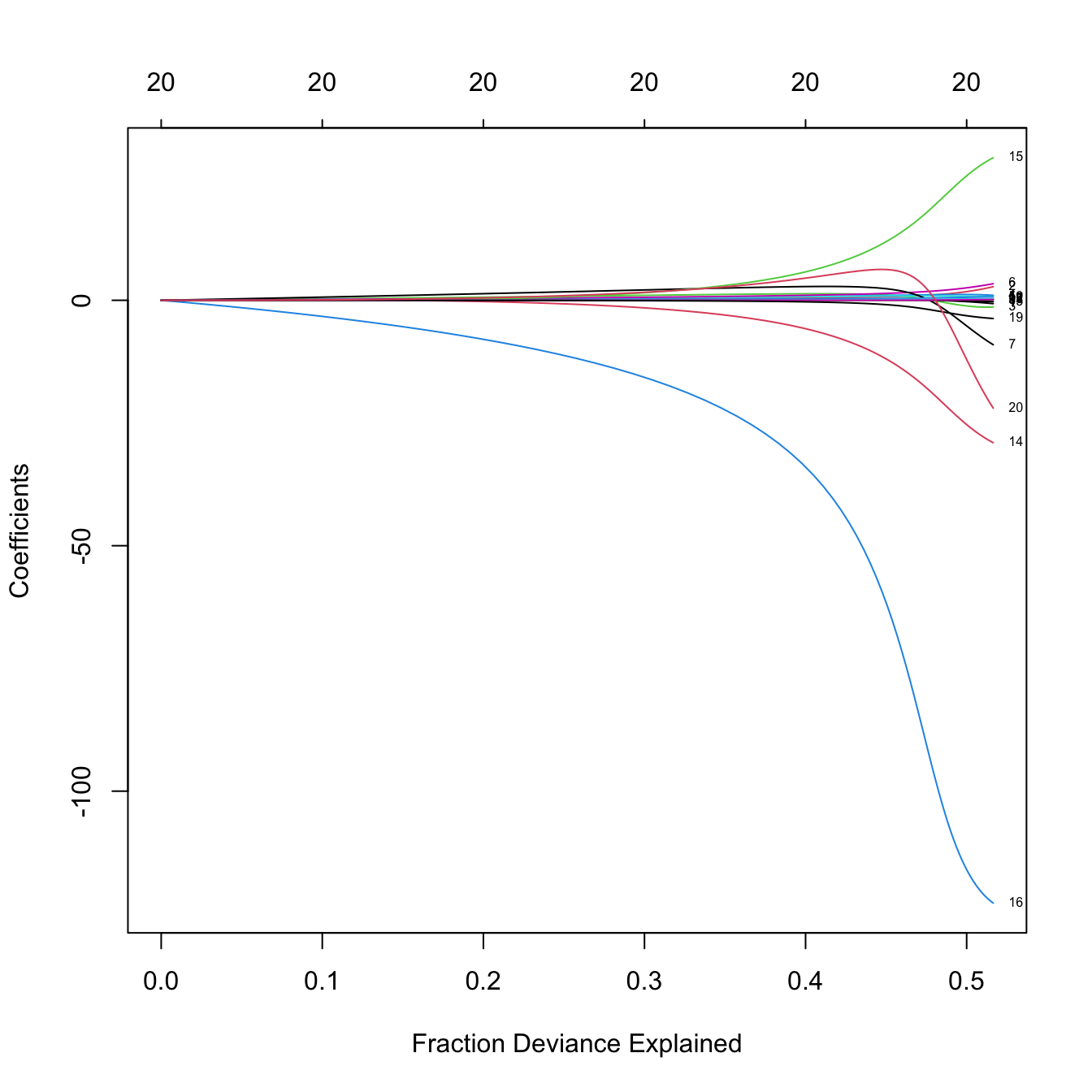
# The maximum R^2 is slightly above 0.5

# Indeed, we can see that R^2 = 0.5461
summary(lm(Salary ~ ., data = Hitters))$r.squared
## [1] 0.5461159

# Some persistently important predictors are 15, 14, and 19
colnames(x)[c(15, 14, 19)]
## [1] "DivisionW"  "LeagueN"    "NewLeagueN"
# Dummies associated to league and division are important

# What is inside glmnet's output?
names(ridge_mod)
##  [1] "a0"        "beta"      "df"        "dim"       "lambda"    "dev.ratio" "nulldev"   "npasses"   "jerr"
## [10] "offset"    "call"      "nobs"

# lambda versus R^2 -- fitness decreases when sparsity is introduced, in
# in exchange of better variable interpretation and avoidance of overfitting
plot(-log(ridge_mod$lambda), ridge_mod$dev.ratio, type = "l",
     xlab = "-log(lambda)", ylab = "R2")
ridge_mod$dev.ratio[length(ridge_mod$dev.ratio)]
## [1] 0.5164455
# Slightly different to lm's because it compromises accuracy for speed

# The coefficients for different values of lambda are given in $a0 (intercepts)
# and $beta (slopes) or, alternatively, both in coef(ridgeMod)
length(ridge_mod$a0)
## [1] 100
dim(ridge_mod$beta)
## [1]  19 100
length(ridge_mod$lambda) # 100 lambda's were automatically chosen
## [1] 100

# Estimated coefficients for the 50th value of lambda (includes intercept also)
coef(ridge_mod)[, 50]
##   (Intercept)         AtBat          Hits         HmRun          Runs           RBI         Walks         Years
## 213.066443434   0.090095728   0.371252756   1.180126956   0.596298287   0.594502390   0.772525466   2.473494238
##        CAtBat         CHits        CHmRun         CRuns          CRBI        CWalks       LeagueN     DivisionW
##   0.007597952   0.029272172   0.217335716   0.058705097   0.060722036   0.058698830   3.276567828 -21.889942619
##       PutOuts       Assists        Errors    NewLeagueN
##   0.052667119   0.007463678  -0.145121336   2.972759126
ridge_mod$lambda[50]
## [1] 2674.375

# Zoom in path solution
plot(ridge_mod, label = TRUE, xvar = "lambda",
     xlim = -log(ridge_mod$lambda[50]) + c(-2, 2), ylim = c(-30, 10))
abline(v = -log(ridge_mod$lambda[50]))
points(rep(-log(ridge_mod$lambda[50]), nrow(ridge_mod$beta)),
       ridge_mod$beta[, 50], pch = 16, col = 1:6)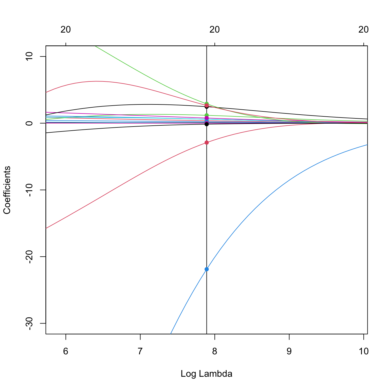
# The squared l2-norm of the coefficients decreases as lambda increases
plot(-log(ridge_mod$lambda), sqrt(colSums(ridge_mod$beta^2)), type = "l",
     xlab = "-log(lambda)", ylab = "l2 norm")
4.1.1.2 Tuning parameter selection
The selection of the penalty parameter \(\lambda\) is usually done by \(k\)-fold cross-validation, following the general principle described at the end of Section 3.6. This data-driven selector is denoted by \(\hat\lambda_{k\text{-CV}}\) and has the form given114 in (3.18) (or (3.17) if \(k=n\)):
\[\begin{align*} \hat{\lambda}_{k\text{-CV}}:=\arg\min_{\lambda\geq0} \text{CV}_k(\lambda),\quad \text{CV}_k(\lambda):=\sum_{j=1}^k \sum_{i\in F_j} (Y_i-\hat m_{\lambda,-F_{j}}(\mathbf{X}_i))^2. \end{align*}\]
A very interesting variant for the \(\hat{\lambda}_{k\text{-CV}}\) selector is the so-called one standard error rule. This rule is based on a parsimonious principle:
“favor simplicity within the set of most likely optimal models”.
It arises from observing that the objective function to minimize, \(\text{CV}_k,\) is random. Thus, its minimizer \(\hat{\lambda}_{k\text{-CV}}\) is subjected to variability. Then, the parsimonious approach proceeds by selecting not \(\hat{\lambda}_{k\text{-CV}},\) but the largest \(\lambda\) (hence, the simplest model) that is still likely optimal, i.e., that is “close” to \(\hat{\lambda}_{k\text{-CV}}.\) This closeness is quantified by the estimation of the standard deviation of the random variable \(\text{CV}_k(\hat\lambda_{k\text{-CV}}),\) which is obtained thanks to the folding splitting of the sample. Equivalently, \(\hat\lambda_{k\text{-1SE}}\) selects the simplest model whose CV error is not “significantly” worse than that of the model chosen by \(\hat\lambda_{k\text{-CV}}.\)115 Mathematically, \(\hat\lambda_{k\text{-1SE}}\) is defined as
\[\begin{align*} \hat\lambda_{k\text{-1SE}}:=\max\left\{\lambda\geq 0 : \text{CV}_k(\lambda)\in\left(\text{CV}_k(\hat\lambda_{k\text{-CV}})\pm\hat{\mathrm{SE}}\left(\text{CV}_k(\hat\lambda_{k\text{-CV}})\right)\right)\right\}. \end{align*}\]
The \(\hat\lambda_{k\text{-1SE}}\) selector often offers a good trade-off between model fitness and interpretability in practice.116 The code below gives all the details.
# If we want, we can choose manually the grid of penalty parameters to explore
# The grid should be descending
ridge_mod2 <- glmnet(x = x, y = y, alpha = 0, lambda = 100:1)
plot(ridge_mod2, label = TRUE, xvar = "lambda") # Not a good choice!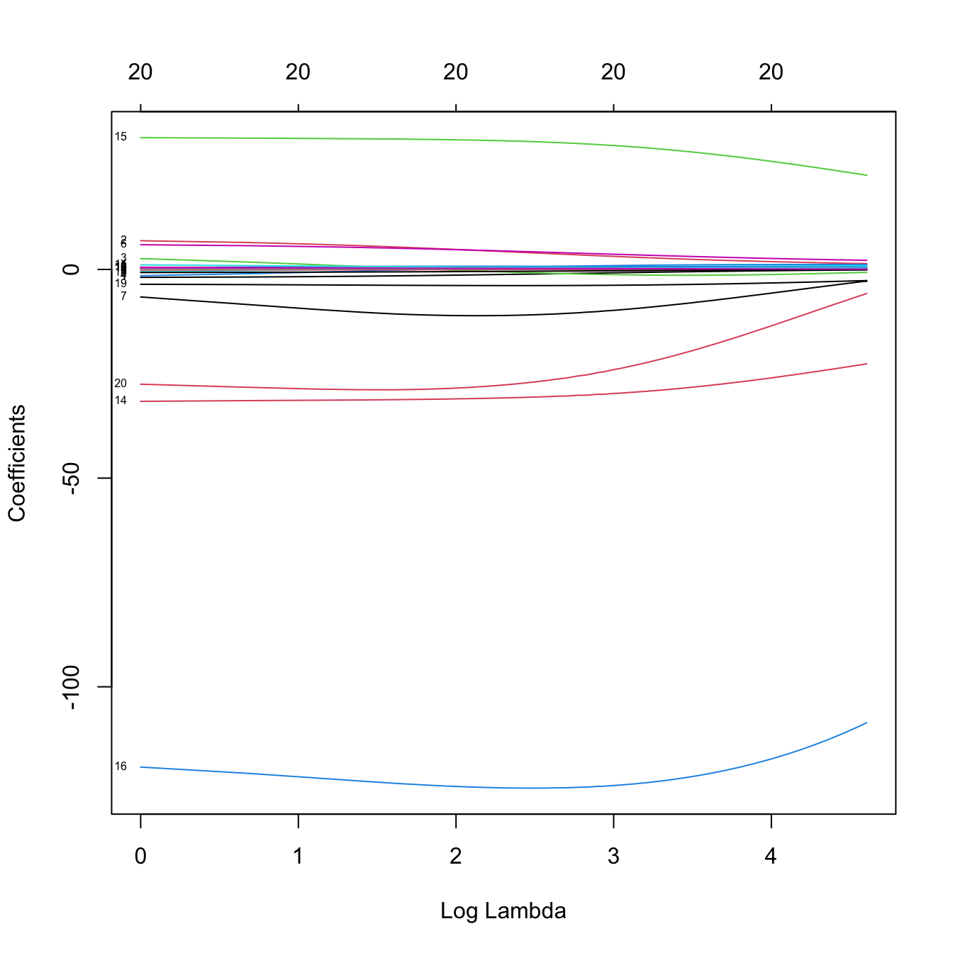
# Lambda is a tuning parameter that can be chosen by cross-validation, using as
# error the MSE (other possible error can be considered for generalized models
# using the argument type.measure)

# 10-fold cross-validation. Change the seed for a different result
set.seed(12345)
kcv_ridge <- cv.glmnet(x = x, y = y, alpha = 0, nfolds = 10)

# The lambda that minimizes the CV error is
kcv_ridge$lambda.min
## [1] 25.52821

# Equivalent to
ind_min <- which.min(kcv_ridge$cvm)
kcv_ridge$lambda[ind_min]
## [1] 25.52821

# The minimum CV error
kcv_ridge$cvm[ind_min]
## [1] 114989.5
min(kcv_ridge$cvm)
## [1] 114989.5

# Potential problem! Minimum occurs at one extreme of the lambda grid in which
# CV is done. The grid was automatically selected, but can be manually inputted
range(kcv_ridge$lambda)
## [1]     25.52821 255282.09651
lambda_grid <- 10^seq(log10(kcv_ridge$lambda[1]), log10(0.1),
                      length.out = 150) # log-spaced grid
kcv_ridge2 <- cv.glmnet(x = x, y = y, nfolds = 10, alpha = 0,
                        lambda = lambda_grid)

# Much better
plot(kcv_ridge2)
kcv_ridge2$lambda.min
## [1] 9.506186

# But the CV curve is random, since it depends on the sample. Its variability
# can be estimated by considering the CV curves of each fold. An alternative
# approach to select lambda is to choose the largest within one standard
# deviation of the minimum error, in order to favor simplicity of the model
# around the optimal lambda value. This is known as the "one standard error rule"
kcv_ridge2$lambda.1se
## [1] 2964.928

# Location of both optimal lambdas in the CV loss function in dashed vertical
# lines, and lowest CV error and lowest CV error + one standard error
plot(kcv_ridge2)
ind_min2 <- which.min(kcv_ridge2$cvm)
abline(h = kcv_ridge2$cvm[ind_min2] + c(0, kcv_ridge2$cvsd[ind_min2]))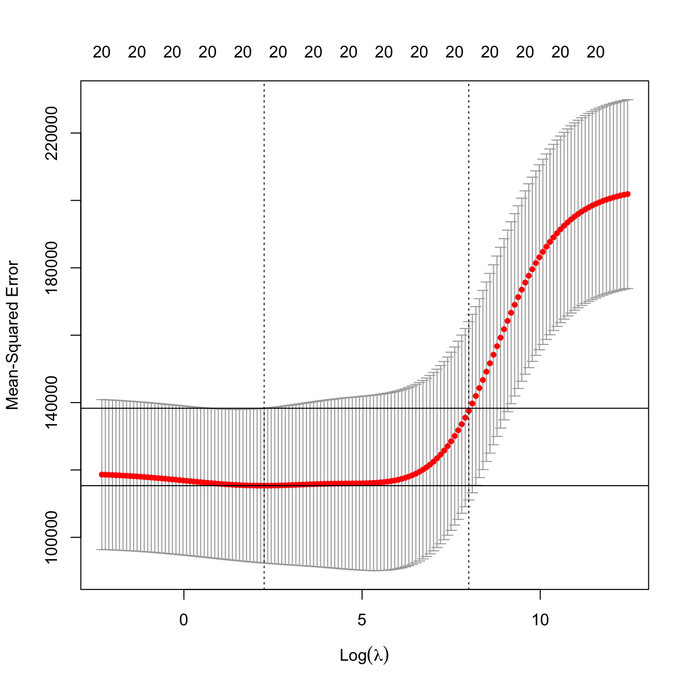
# The consideration of the one standard error rule for selecting lambda makes
# special sense when the CV function is quite flat around the minimum (hence an
# overpenalization that gives more sparsity does not affect so much the CV loss)

# Leave-one-out cross-validation. More computationally intense but completely
# objective in the choice of the fold-assignment
ncv_ridge <- cv.glmnet(x = x, y = y, alpha = 0, nfolds = nrow(Hitters),
                       lambda = lambda_grid)

# Location of both optimal lambdas in the CV loss function
plot(ncv_ridge)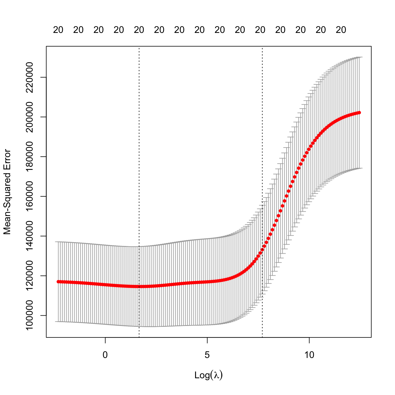
# By default, cv.glmnet randomly allocates observations to folds. Passing foldid
# uses the supplied partition instead to enable running cv.glmnet several times
# on the same folds so that the CV errors are directly comparable. Must be a
# vector of length n with integer fold labels in 1:nfolds
foldid <- sample(rep(1:10, length.out = nrow(Hitters)))
kcv_ridge_foldid <- cv.glmnet(x = x, y = y, alpha = 0, foldid = foldid,
                              lambda = lambda_grid)
kcv_lasso_foldid <- cv.glmnet(x = x, y = y, alpha = 1, foldid = foldid,
                              lambda = lambda_grid)

# Minimum CV errors are comparable because they come from the same folds
min(kcv_ridge_foldid$cvm)
## [1] 111087.3
min(kcv_lasso_foldid$cvm)
## [1] 110834.9
4.1.1.3 Prediction
# Inspect the best models (the glmnet fit is inside the output of cv.glmnet)
plot(kcv_ridge2$glmnet.fit, label = TRUE, xvar = "lambda")
abline(v = -log(c(kcv_ridge2$lambda.min, kcv_ridge2$lambda.1se)))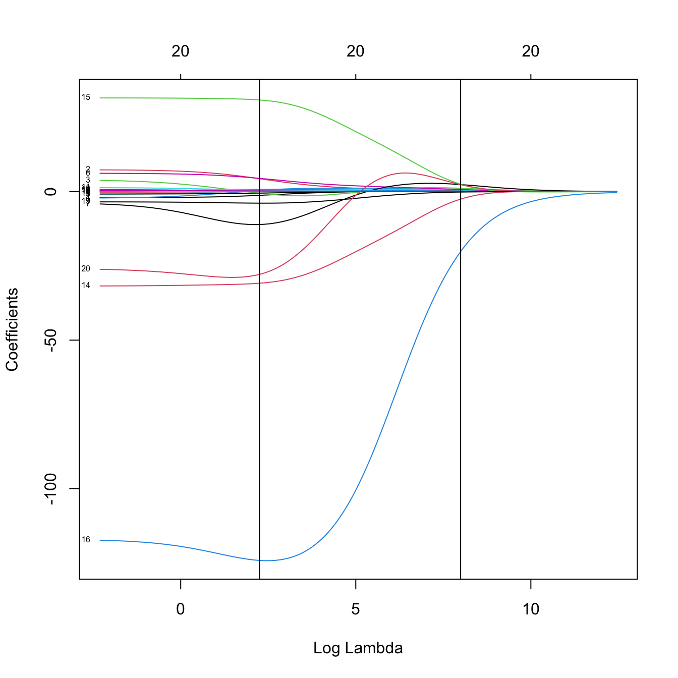
# The fit associated with lambda.1se (or any other lambda not included in the
# original path solution -- obtained by an interpolation) can be retrieved with
# coef() (includes intercept also)
coef(kcv_ridge2, s = kcv_ridge2$lambda.1se)
## 20 x 1 sparse Matrix of class "dgCMatrix"
##                s=2964.928
## (Intercept) 228.344775043
## AtBat         0.086230894
## Hits          0.350997307
## HmRun         1.140159815
## Runs          0.566431889
## RBI           0.567402178
## Walks         0.731035996
## Years         2.388794241
## CAtBat        0.007261907
## CHits         0.027856463
## CHmRun        0.207108274
## CRuns         0.055868452
## CRBI          0.057771696
## CWalks        0.056352942
## LeagueN       2.806441919
## DivisionW   -20.165191961
## PutOuts       0.048940708
## Assists       0.007020284
## Errors       -0.126333988
## NewLeagueN    2.620800863

# Alternatively, one can use
predict(kcv_ridge2, type = "coefficients", s = kcv_ridge2$lambda.1se)
## 20 x 1 sparse Matrix of class "dgCMatrix"
##                s=2964.928
## (Intercept) 228.344775043
## AtBat         0.086230894
## Hits          0.350997307
## HmRun         1.140159815
## Runs          0.566431889
## RBI           0.567402178
## Walks         0.731035996
## Years         2.388794241
## CAtBat        0.007261907
## CHits         0.027856463
## CHmRun        0.207108274
## CRuns         0.055868452
## CRBI          0.057771696
## CWalks        0.056352942
## LeagueN       2.806441919
## DivisionW   -20.165191961
## PutOuts       0.048940708
## Assists       0.007020284
## Errors       -0.126333988
## NewLeagueN    2.620800863

# Predictions for the first two observations
predict(kcv_ridge2, type = "response", s = kcv_ridge2$lambda.1se,
        newx = x[1:2, ])
##              s=2964.928
## -Alan Ashby    529.8402
## -Alvin Davis   578.7483

# Predictions for the first observation, for all the lambdas. We can see how
# the prediction for one observation changes according to lambda
plot(-log(kcv_ridge2$lambda),
     predict(kcv_ridge2, type = "response", newx = x[1, , drop = FALSE],
             s = kcv_ridge2$lambda),
     type = "l", xlab = "-log(lambda)", ylab = " Prediction")
4.1.1.4 Analytical form
The optimization problem (4.5) has an explicit solution for \(\alpha=0.\) To see it, assume that both the response \(Y\) and the predictors \(X_1,\ldots,X_p\) are centered, and that the sample \(\{(\mathbf{X}_i,Y_i)\}_{i=1}^n\) is also centered.117 In this case, there is no intercept \(\beta_0\) (\(=0\)) to estimate by \(\hat\beta_0\) (\(=0\)) and the linear model is simply
\[\begin{align*} Y=\beta_1X_1+\cdots+\beta_pX_p+\varepsilon. \end{align*}\]
Then, the ridge regression estimator \(\hat{\boldsymbol{\beta}}_{\lambda,0}\in\mathbb{R}^p\) is
\[\begin{align} \hat{\boldsymbol{\beta}}_{\lambda,0}&=\arg\min_{\boldsymbol{\beta}\in\mathbb{R}^{p}}\text{RSS}(\boldsymbol{\beta})+\lambda\|\boldsymbol\beta\|_2^2\nonumber\\ &=\arg\min_{\boldsymbol{\beta}\in\mathbb{R}^{p}}\sum_{i=1}^n(Y_i-\mathbf{X}_i\boldsymbol{\beta})^2+\lambda\boldsymbol\beta^\top\boldsymbol\beta\nonumber\\ &=\arg\min_{\boldsymbol{\beta}\in\mathbb{R}^{p}}(\mathbf{Y}-\mathbb{X}\boldsymbol{\beta})^\top(\mathbf{Y}-\mathbb{X}\boldsymbol{\beta})+\lambda\boldsymbol\beta^\top\boldsymbol\beta,\tag{4.7} \end{align}\]
where \(\mathbb{X}\) is the design matrix but now excluding the column of ones (thus of size \(n\times p\)). Nicely, (4.7) is a continuous quadratic optimization problem that is easily solved with the same arguments we employed for obtaining (2.7), resulting in118
\[\begin{align} \hat{\boldsymbol{\beta}}_{\lambda,0}=(\mathbb{X}^\top\mathbb{X}+\lambda\mathbf{I}_p)^{-1}\mathbb{X}^\top\mathbf{Y}.\tag{4.8} \end{align}\]
The form (4.8) neatly connects with the least squares estimator (\(\lambda=0\)) and yields many interesting insights. First, notice how the ridge regression estimator is always computable, even if \(p\gg n\;\)119 and the matrix \(\mathbb{X}^\top\mathbb{X}\) is not invertible, or if \(\mathbb{X}^\top\mathbb{X}\) is singular due to perfect multicollinearity. Second, as it was done with (2.11), it is straightforward to see that, under the assumptions of the linear model,
\[\begin{align} \hat{\boldsymbol{\beta}}_{\lambda,0}\sim\mathcal{N}_{p}\left((\mathbb{X}^\top\mathbb{X}+\lambda\mathbf{I}_p)^{-1}\mathbb{X}^\top\mathbb{X}\boldsymbol{\beta},\sigma^2(\mathbb{X}^\top\mathbb{X}+\lambda\mathbf{I}_p)^{-1}\mathbb{X}^\top\mathbb{X}(\mathbb{X}^\top\mathbb{X}+\lambda\mathbf{I}_p)^{-1}\right).\tag{4.9} \end{align}\]
The distribution (4.9) is revealing: it shows that \(\hat{\boldsymbol{\beta}}_{\lambda,0}\) is no longer unbiased and that its variance is smaller120 than the least squares estimator \(\hat{\boldsymbol{\beta}}.\) This is much more clear in the case where the predictors are also uncorrelated and standardized (in addition to being centered), hence the sample covariance matrix is \(\mathbf{S}=\mathbf{I}_p\) and, equivalently, \(\mathbb{X}^\top\mathbb{X}=n\mathbf{I}_p.\) This is precisely the case of the PCA or PLS scores if these are standardized to have unit variance. In this situation, then (4.8) and (4.9) simplify to121
\[\begin{align} \begin{split} \hat{\boldsymbol{\beta}}_{\lambda,0}&=\frac{1}{n+\lambda}\mathbb{X}^\top\mathbf{Y}=\frac{n}{n+\lambda}\hat{\boldsymbol{\beta}},\\ \hat{\boldsymbol{\beta}}_{\lambda,0}&\sim\mathcal{N}_{p}\left(\frac{n}{n+\lambda}\boldsymbol{\beta},\sigma^2\frac{n}{(n+\lambda)^2}\mathbf{I}_p\right). \end{split} \tag{4.10} \end{align}\]
The shrinking effect of \(\lambda\) is yet more evident from (4.10): when the predictors are uncorrelated, we shrink equally the least squares estimator \(\hat{\boldsymbol{\beta}}\) by the factor \(n/(n+\lambda),\) which results in a reduction of the variance by a factor of \(n/(n+\lambda)^{2}.\) Furthermore, notice an important point: due to the explicit control of the distribution of \(\hat{\boldsymbol{\beta}}_{\lambda,0},\) inference about \(\boldsymbol{\beta}\) can be done in a relatively straightforward way in this special case122 from \(\hat{\boldsymbol{\beta}}_{\lambda,0},\) just as it was done from \(\hat{\boldsymbol{\beta}}\) in Section 2.4. This tractability, both on the explicit form of the estimator and on the associated inference, is one of the main advantages of ridge regression with respect to other shrinkage methods.
Finally, just as we did for the least squares estimator, we can define the hat matrix
\[\begin{align*} \mathbf{H}_\lambda:=\mathbb{X}(\mathbb{X}^\top\mathbb{X}+\lambda\mathbf{I}_p)^{-1}\mathbb{X}^\top \end{align*}\]
that predicts \(\hat{\mathbf{Y}}\) from \(\mathbf{Y}.\) This hat matrix becomes especially useful now, as it can be employed to define the effective degrees of freedom associated with a ridge regression with penalty \(\lambda.\) These are defined as the trace of the hat matrix:
\[\begin{align*} \mathrm{df}(\lambda):=\mathrm{tr}(\mathbf{H}_\lambda). \end{align*}\]
The motivation behind is that, for the unrestricted least squares fit123
\[\begin{align*} \mathrm{tr}(\mathbf{H}_0)=\mathrm{tr}\big(\mathbb{X}(\mathbb{X}^\top\mathbb{X})^{-1}\mathbb{X}^\top\big)=\mathrm{tr}\big(\mathbb{X}^\top\mathbb{X}(\mathbb{X}^\top\mathbb{X})^{-1}\big)=p \end{align*}\]
and thus indeed \(\mathrm{df}(0)=p\) is representing the degrees of freedom of the fit, understood as the number of parameters employed (keep in mind that the intercept was excluded). For a constrained fit with \(\lambda>0,\) \(\mathrm{df}(\lambda)<p\) because, even if we are estimating \(p\) parameters in \(\hat{\boldsymbol{\beta}}_{\lambda,0},\) these are restricted to satisfy \(\|\hat{\boldsymbol{\beta}}_{\lambda,0}\|^2_2\leq s_\lambda\) (for a certain \(s_\lambda,\) recall (4.6)). The function \(\mathrm{df}\) is monotonically decreasing and such that \(\lim_{\lambda\to\infty}\mathrm{df}(\lambda)=0,\) see Figure 4.5. Recall that, due to the imposed constraint on the coefficients, we could choose \(\lambda\) such that \(\mathrm{df}(\lambda)=r,\) where \(r\) is an integer smaller than \(p\): this would correspond to effectively employing exactly \(r\) parameters in the regression, despite considering \(p\) predictors.

Figure 4.5: The effective degrees of freedom \(\mathrm{df}(\lambda)\) as a function of \(-\log(\lambda)\) for a ridge regression with \(p=5.\)
The next chunk of code implements \(\hat{\boldsymbol{\beta}}_{\lambda,0}\) and shows that is equivalent to the output of glmnet::glmnet, with certain quirks.124 \(\!\!^,\)125
# Random data
p <- 5
n <- 200
beta <- seq(-1, 1, l = p)
set.seed(123124)
x <- matrix(rnorm(n * p), n, p)
y <- 1 + x %*% beta + rnorm(n)

# Mimic internal standardization of y done in glmnet, which affects the scale
# of lambda in the regularization
y <- scale(y, center = TRUE, scale = TRUE) * sqrt(n / (n - 1))

# Unrestricted fit
fit <- glmnet(x, y, alpha = 0, lambda = 0, intercept = TRUE,
              standardize = FALSE)
beta0_hat <- rbind(fit$a0, fit$beta)
beta0_hat
## 6 x 1 sparse Matrix of class "dgCMatrix"
##              s0
##    -0.007815871
## V1 -0.521693181
## V2 -0.288052685
## V3 -0.019294336
## V4  0.239902118
## V5  0.535110595

# Unrestricted fit matches least squares -- but recall glmnet uses an
# iterative method so it is inexact (convergence threshold thresh = 1e-7 by
# default)
X <- model.matrix(y ~ x) # A way of constructing a design matrix that is a
# data.frame and has a column of ones
solve(crossprod(X)) %*% t(X) %*% y
##                     [,1]
## (Intercept) -0.007815868
## x1          -0.521693158
## x2          -0.288052685
## x3          -0.019294338
## x4           0.239902117
## x5           0.535110595

# Restricted fit
# glmnet considers as the regularization parameter "lambda" the value
# lambda / n (lambda being here the penalty parameter employed in the theory)
lambda <- 2
fit <- glmnet(x, y, alpha = 0, lambda = lambda / n, intercept = TRUE,
              standardize = FALSE, thresh = 1e-10)
beta_lambda_hat <- rbind(fit$a0, fit$beta)
beta_lambda_hat
## 6 x 1 sparse Matrix of class "dgCMatrix"
##              s0
##    -0.007775041
## V1 -0.517108905
## V2 -0.285489929
## V3 -0.018898839
## V4  0.236836125
## V5  0.530343255

# Analytical form with intercept
solve(crossprod(X) + diag(c(0, rep(lambda, p)))) %*% t(X) %*% y
##                     [,1]
## (Intercept) -0.007775041
## x1          -0.517108905
## x2          -0.285489929
## x3          -0.018898839
## x4           0.236836125
## x5           0.530343255
4.1.2 Lasso
The main novelty in lasso with respect to ridge is its ability to exactly zero coefficients and the lack of analytical solution. Fitting, tuning parameter selection, and prediction are completely analogous to ridge regression.
4.1.2.1 Fitting
# Get the Hitters data back
Hitters <- na.omit(Hitters)
x <- model.matrix(Salary ~ ., data = Hitters)[, -1]
y <- Hitters$Salary

# Call to the main function -- use alpha = 1 for lasso regression (the default)
lasso_mod <- glmnet(x = x, y = y, alpha = 1)
# Same defaults as before, same object structure

# Plot of the solution path -- now the paths are not smooth when decreasing to
# zero (they are zero exactly). This is a consequence of the l1 norm
plot(lasso_mod, xvar = "lambda", label = TRUE)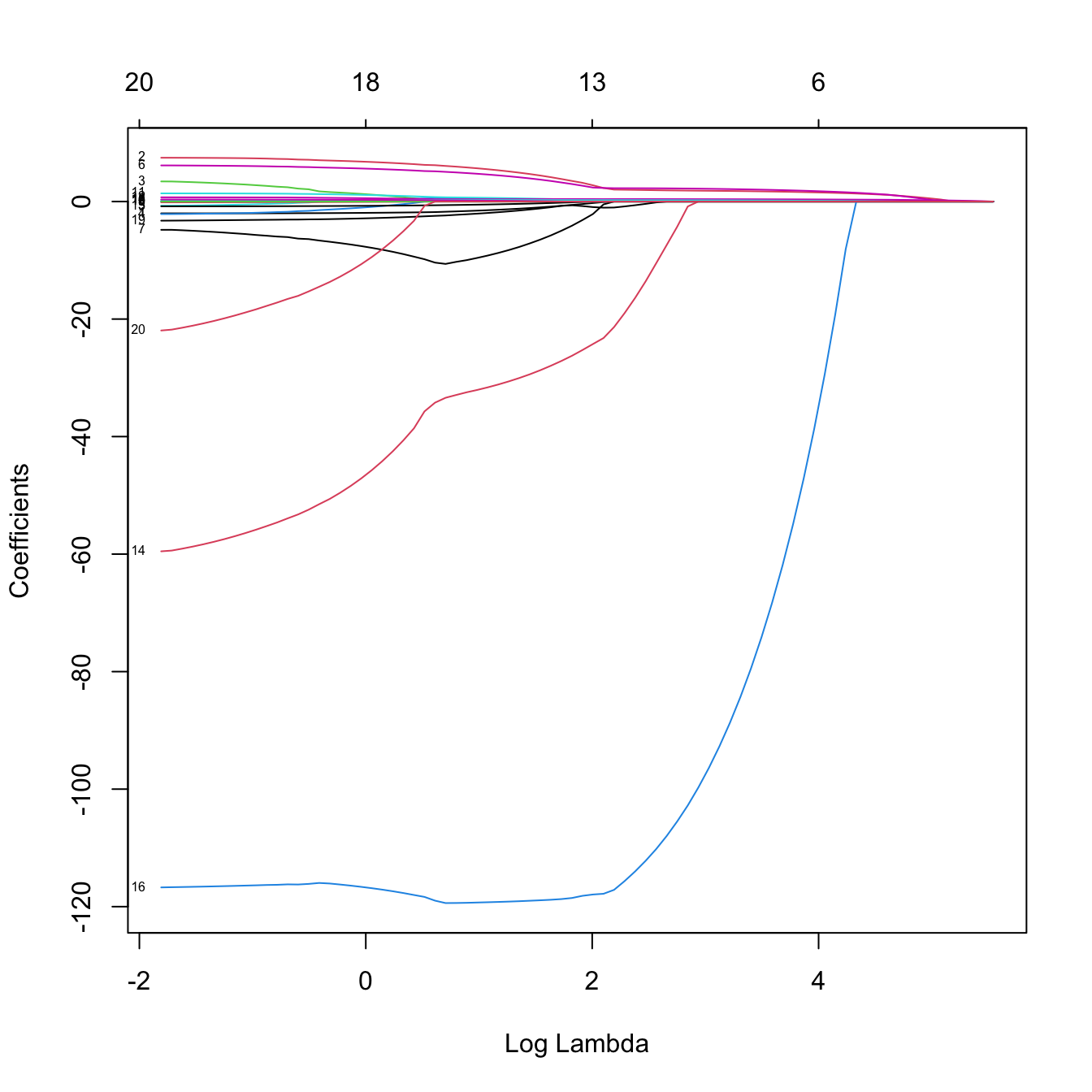
# Some persistently important predictors are 15, 14, and 19
colnames(x)[c(15, 14, 19)]
## [1] "DivisionW"  "LeagueN"    "NewLeagueN"
# Dummies associated to league and division are important

# Versus the R^2 -- same maximum R^2 as before
plot(lasso_mod, label = TRUE, xvar = "dev")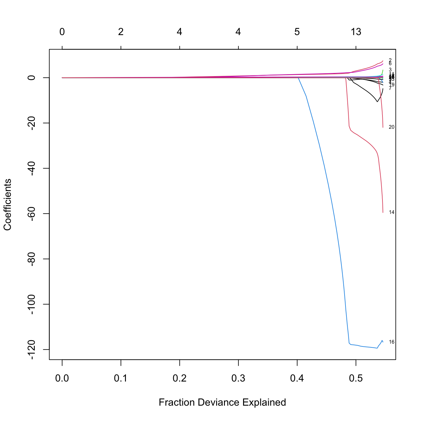
# Now the l1-norm of the coefficients decreases as lambda increases
plot(-log(lasso_mod$lambda), colSums(abs(lasso_mod$beta)), type = "l",
     xlab = "-log(lambda)", ylab = "l1 norm")
# 10-fold cross-validation. Change the seed for a different result
set.seed(12345)
kcv_lasso <- cv.glmnet(x = x, y = y, alpha = 1, nfolds = 10)

# The lambda that minimizes the CV error
kcv_lasso$lambda.min
## [1] 2.674375

# The "one standard error rule" for lambda
kcv_lasso$lambda.1se
## [1] 76.16717

# Location of both optimal lambdas in the CV loss function
ind_min <- which.min(kcv_lasso$cvm)
plot(kcv_lasso)
abline(h = kcv_lasso$cvm[ind_min] + c(0, kcv_lasso$cvsd[ind_min]))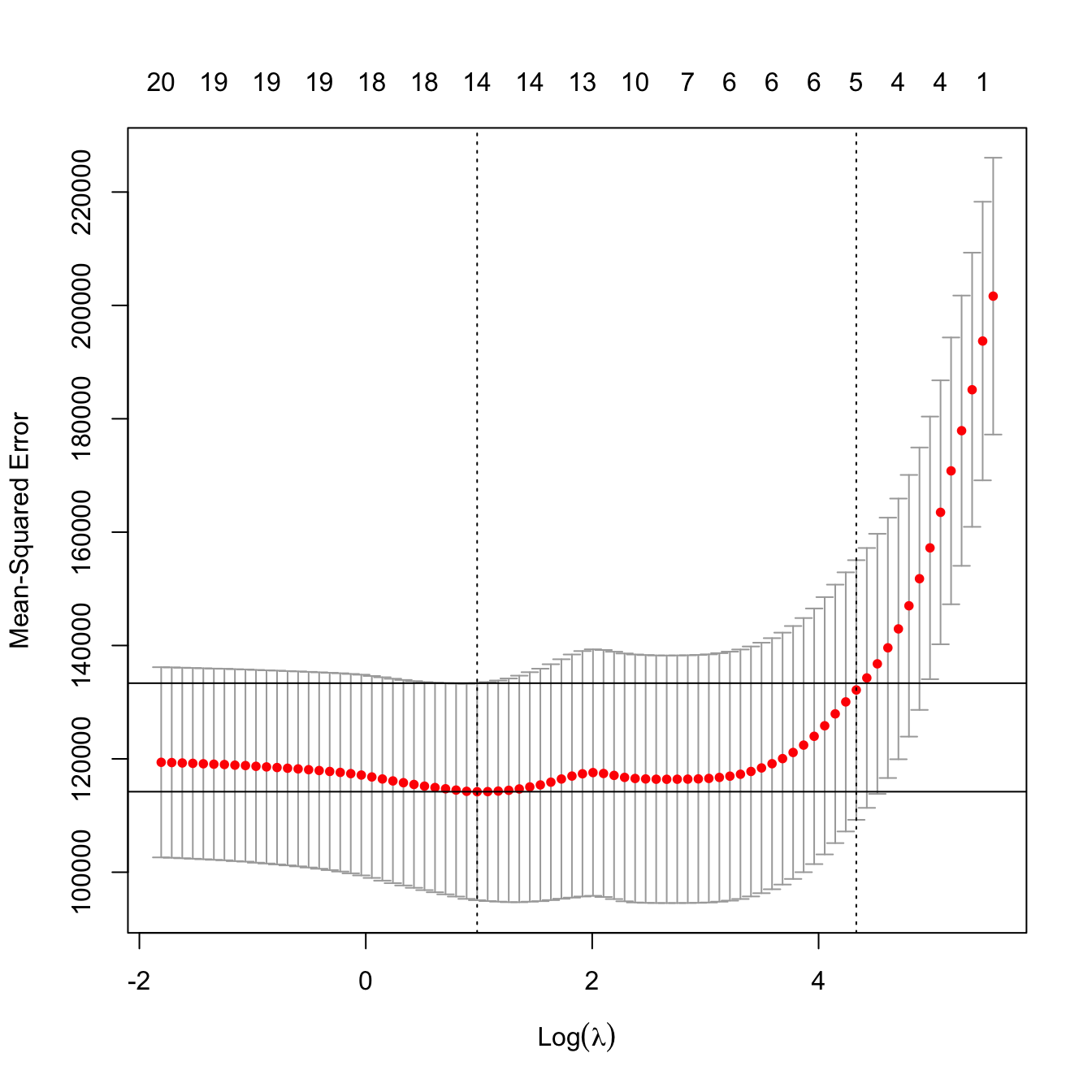
# No problems now: the minimum does not occur at one extreme
# Interesting: note that the numbers on top of the figure give the number of
# coefficients *exactly* different from zero -- the number of predictors
# effectively considered in the model!
# In this case, the one standard error rule makes also sense

# Leave-one-out cross-validation
lambda_grid <- 10^seq(log10(kcv_lasso$lambda[1]), log10(0.1),
                      length.out = 150) # log-spaced grid
ncv_lasso <- cv.glmnet(x = x, y = y, alpha = 1, nfolds = nrow(Hitters),
                       lambda = lambda_grid)

# Location of both optimal lambdas in the CV loss function
plot(ncv_lasso)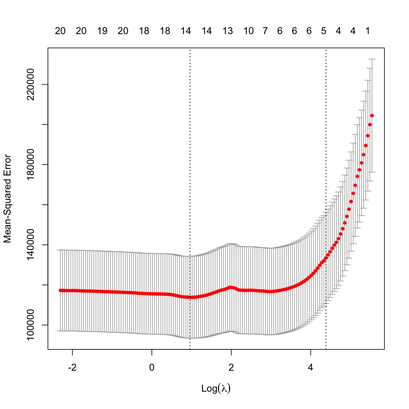
4.1.2.2 Prediction
# Inspect the best models
plot(kcv_lasso$glmnet.fit, label = TRUE, xvar = "lambda")
abline(v = -log(c(kcv_lasso$lambda.min, kcv_lasso$lambda.1se)))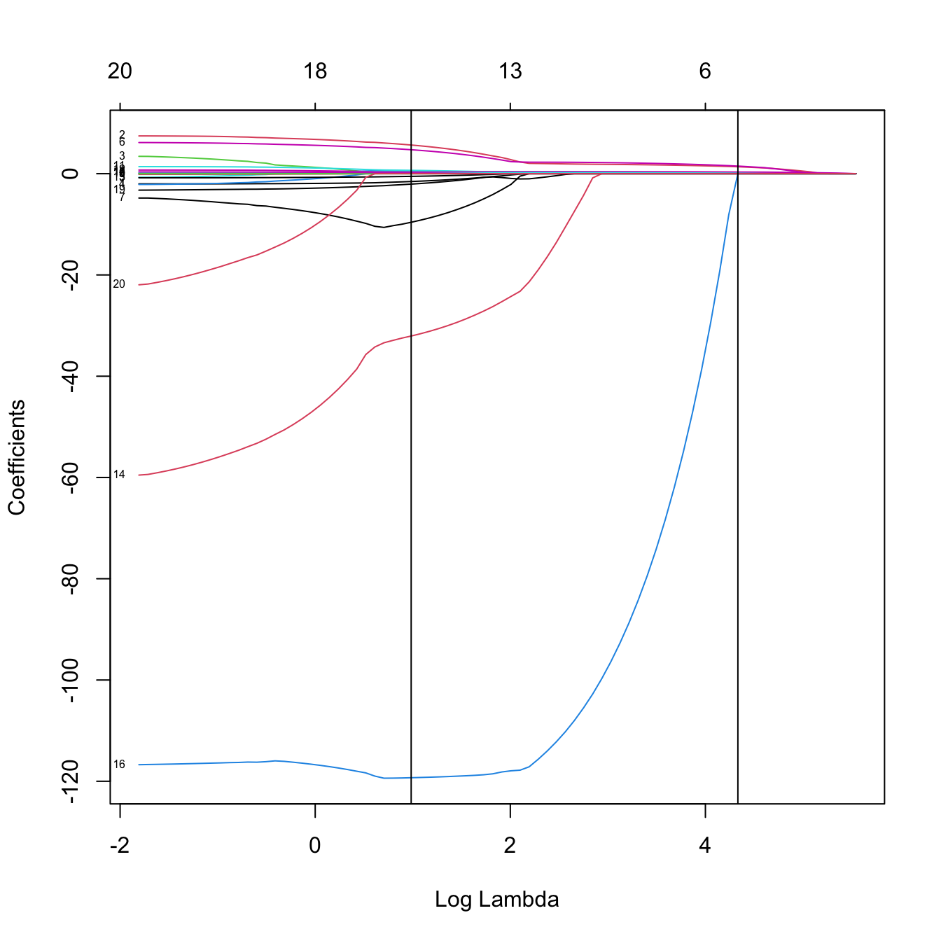
# The model associated with lambda.min (or any other lambda not included in the
# original path solution -- obtained by an interpolation) can be retrieved with
coef(kcv_lasso, s = c(kcv_lasso$lambda.min, kcv_lasso$lambda.1se))
## 20 x 2 sparse Matrix of class "dgCMatrix"
##              s= 2.674375  s=76.167172
## (Intercept)  123.7520756 144.37970458
## AtBat         -1.5473426   .
## Hits           5.6608972   1.36380384
## HmRun          .           .
## Runs           .           .
## RBI            .           .
## Walks          4.7296908   1.49731098
## Years         -9.5958375   .
## CAtBat         .           .
## CHits          .           .
## CHmRun         0.5108207   .
## CRuns          0.6594856   0.15275165
## CRBI           0.3927505   0.32833941
## CWalks        -0.5291586   .
## LeagueN       32.0650811   .
## DivisionW   -119.2990171   .
## PutOuts        0.2724045   0.06625755
## Assists        0.1732025   .
## Errors        -2.0585083   .
## NewLeagueN     .           .

# Predictions for the first two observations
predict(kcv_lasso, type = "response",
        s = c(kcv_lasso$lambda.min, kcv_lasso$lambda.1se),
        newx = x[1:2, ])
##              s= 2.674375 s=76.167172
## -Alan Ashby     427.8822    540.0835
## -Alvin Davis    700.1705    615.3311
4.1.3 Variable selection with lasso
Thanks to its ability to exactly zeroing coefficients, lasso is a powerful device for performing variable/model selection within its fit. The practical approach is really simple and amounts to identify the entries of \(\hat{\boldsymbol{\beta}}_{\lambda,1}\) different from zero, after \(\lambda\) is appropriately selected.
# We can use lasso for model selection!
sel_preds <- coef(kcv_lasso, s = c(kcv_lasso$lambda.min,
                                   kcv_lasso$lambda.1se))[-1, ] != 0
x1 <- x[, sel_preds[, 1]]
x2 <- x[, sel_preds[, 2]]

# Least squares fit with variables selected by lasso
mod_lasso_sel1 <- lm(y ~ x1)
mod_lasso_sel2 <- lm(y ~ x2)
summary(mod_lasso_sel1)
##
## Call:
## lm(formula = y ~ x1)
##
## Residuals:
##     Min      1Q  Median      3Q     Max
## -940.10 -174.20  -25.94  127.05 1890.12
##
## Coefficients:
##               Estimate Std. Error t value Pr(>|t|)
## (Intercept)  187.55948   88.57177   2.118 0.035200 *
## x1AtBat       -2.30798    0.56236  -4.104  5.5e-05 ***
## x1Hits         7.34602    1.71760   4.277  2.7e-05 ***
## x1Walks        6.08610    1.57008   3.876 0.000136 ***
## x1Years      -13.60502   10.38333  -1.310 0.191310
## x1CHmRun       0.83633    0.84709   0.987 0.324457
## x1CRuns        0.90924    0.27662   3.287 0.001159 **
## x1CRBI         0.35734    0.36252   0.986 0.325229
## x1CWalks      -0.83918    0.27207  -3.084 0.002270 **
## x1LeagueN     36.68460   40.73468   0.901 0.368685
## x1DivisionW -119.67399   39.32485  -3.043 0.002591 **
## x1PutOuts      0.29296    0.07632   3.839 0.000157 ***
## x1Assists      0.31483    0.20460   1.539 0.125142
## x1Errors      -3.23219    4.29443  -0.753 0.452373
## ---
## Signif. codes:  0 '***' 0.001 '**' 0.01 '*' 0.05 '.' 0.1 ' ' 1
##
## Residual standard error: 314 on 249 degrees of freedom
## Multiple R-squared:  0.5396, Adjusted R-squared:  0.5156
## F-statistic: 22.45 on 13 and 249 DF,  p-value: < 2.2e-16
summary(mod_lasso_sel2)
##
## Call:
## lm(formula = y ~ x2)
##
## Residuals:
##     Min      1Q  Median      3Q     Max
## -914.21 -171.94  -33.26   97.63 2197.08
##
## Coefficients:
##              Estimate Std. Error t value Pr(>|t|)
## (Intercept) -96.96096   55.62583  -1.743 0.082513 .
## x2Hits        2.09338    0.57376   3.649 0.000319 ***
## x2Walks       2.51513    1.22010   2.061 0.040269 *
## x2CRuns       0.26490    0.19463   1.361 0.174679
## x2CRBI        0.39549    0.19755   2.002 0.046339 *
## x2PutOuts     0.26620    0.07857   3.388 0.000814 ***
## ---
## Signif. codes:  0 '***' 0.001 '**' 0.01 '*' 0.05 '.' 0.1 ' ' 1
##
## Residual standard error: 333 on 257 degrees of freedom
## Multiple R-squared:  0.4654, Adjusted R-squared:  0.455
## F-statistic: 44.75 on 5 and 257 DF,  p-value: < 2.2e-16

# Comparison with stepwise selection
mod_bic <- step(lm(Salary ~ ., data = Hitters), k = log(nrow(Hitters)),
                trace = 0)
summary(mod_bic)
##
## Call:
## lm(formula = Salary ~ AtBat + Hits + Walks + CRuns + CRBI + CWalks +
##     Division + PutOuts, data = Hitters)
##
## Residuals:
##     Min      1Q  Median      3Q     Max
## -794.06 -171.94  -28.48  133.36 2017.83
##
## Coefficients:
##               Estimate Std. Error t value Pr(>|t|)
## (Intercept)  117.15204   65.07016   1.800 0.072985 .
## AtBat         -2.03392    0.52282  -3.890 0.000128 ***
## Hits           6.85491    1.65215   4.149 4.56e-05 ***
## Walks          6.44066    1.52212   4.231 3.25e-05 ***
## CRuns          0.70454    0.24869   2.833 0.004981 **
## CRBI           0.52732    0.18861   2.796 0.005572 **
## CWalks        -0.80661    0.26395  -3.056 0.002483 **
## DivisionW   -123.77984   39.28749  -3.151 0.001824 **
## PutOuts        0.27539    0.07431   3.706 0.000259 ***
## ---
## Signif. codes:  0 '***' 0.001 '**' 0.01 '*' 0.05 '.' 0.1 ' ' 1
##
## Residual standard error: 314.7 on 254 degrees of freedom
## Multiple R-squared:  0.5281, Adjusted R-squared:  0.5133
## F-statistic: 35.54 on 8 and 254 DF,  p-value: < 2.2e-16
# The lasso variable selection is similar, although the model is slightly worse
# in terms of adjusted R^2 and significance of the predictors. However, keep in
# mind that lasso is solving a constrained least squares problem, so it is
# expected to achieve better R^2 and adjusted R^2 via a selection procedure
# that employs solutions of unconstrained least squares. What is remarkable
# is the speed of lasso on selecting variables, and the fact that gives quite
# good starting points for performing further model selection

# Another interesting possibility is to run a stepwise selection starting from
# the set of predictors selected by lasso. In this search, it is important to
# use direction = "both" (default) and define the scope argument adequately.
# Work on a data frame whose columns ARE the design-matrix predictors (dummies
# included) so that lasso-selected dummy names like "LeagueN" match actual
# columns, and so that factor levels with spaces or unusual characters are
# sanitized into valid R names by data.frame()
hitters_dummies <- data.frame(Salary = y, x)
sel_names <- names(hitters_dummies)[-1][sel_preds[, 2]]
f <- reformulate(termlabels = sel_names, response = "Salary")
start <- lm(f, data = hitters_dummies) # Model with predictors selected by lasso
scope <- list(lower = ~ 1, # No predictors
              upper = terms(Salary ~ ., data = hitters_dummies)) # All preds
mod_bic_from_lasso <- step(object = start, k = log(nrow(hitters_dummies)),
                           scope = scope, trace = 0)
summary(mod_bic_from_lasso)
##
## Call:
## lm(formula = Salary ~ Hits + Walks + CRBI + PutOuts + AtBat +
##     DivisionW, data = hitters_dummies)
##
## Residuals:
##     Min      1Q  Median      3Q     Max
## -873.11 -181.72  -25.91  141.77 2040.47
##
## Coefficients:
##               Estimate Std. Error t value Pr(>|t|)
## (Intercept)   91.51180   65.00006   1.408 0.160382
## Hits           7.60440    1.66254   4.574 7.46e-06 ***
## Walks          3.69765    1.21036   3.055 0.002488 **
## CRBI           0.64302    0.06443   9.979  < 2e-16 ***
## PutOuts        0.26431    0.07477   3.535 0.000484 ***
## AtBat         -1.86859    0.52742  -3.543 0.000470 ***
## DivisionW   -122.95153   39.82029  -3.088 0.002239 **
## ---
## Signif. codes:  0 '***' 0.001 '**' 0.01 '*' 0.05 '.' 0.1 ' ' 1
##
## Residual standard error: 319.9 on 256 degrees of freedom
## Multiple R-squared:  0.5087, Adjusted R-squared:  0.4972
## F-statistic: 44.18 on 6 and 256 DF,  p-value: < 2.2e-16

# Comparison in terms of BIC, slight improvement with mod_bic_from_lasso
BIC(mod_lasso_sel1, mod_lasso_sel2, mod_bic_from_lasso, mod_bic)
##                    df      BIC
## mod_lasso_sel1     15 3839.690
## mod_lasso_sel2      7 3834.434
## mod_bic_from_lasso  8 3817.785
## mod_bic            10 3818.320
Exercise 4.1 Consider la-liga-2015-2016.xlsx dataset. We aim to predict Points after removing the perfectly related linear variables with Points. Do the following:
- Lasso regression. Select \(\lambda\) by cross-validation. Obtain the estimated coefficients for the chosen lambda.
- Use the predictors with non-null coefficients for creating a model with
lm. - Summarize the model and check for multicollinearity.
It may happen that the cross-validation curve has a reverse “L”-shaped form without a well-defined global minimum. This usually happens when only the intercept is significant and none of the predictors are relevant for explaining \(Y.\)
The code below illustrates the previous warning.
# Random data with predictors unrelated to the response
p <- 100
n <- 300
set.seed(123124)
x <- matrix(rnorm(n * p), n, p)
y <- 1 + rnorm(n)

# CV
lambda_grid <- exp(seq(-10, 3, l = 200))
plot(cv.glmnet(x = x, y = y, alpha = 1, nfolds = n, lambda = lambda_grid))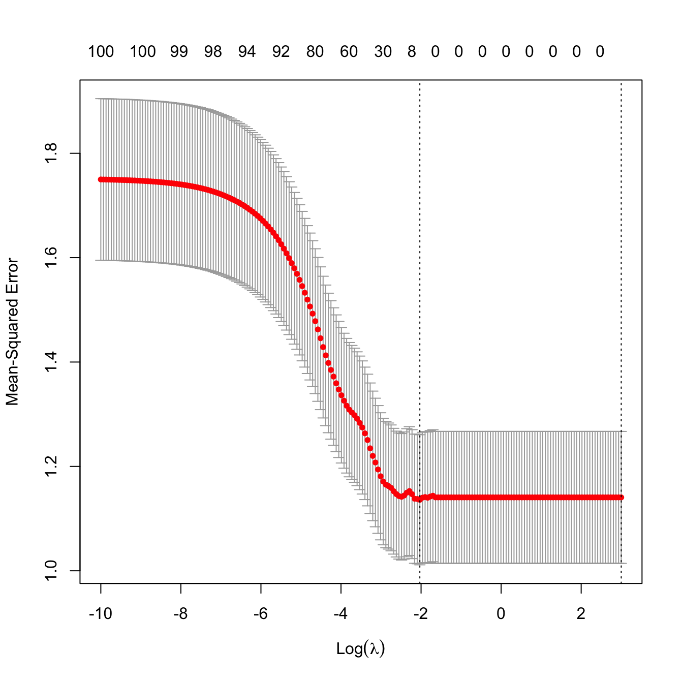
Figure 4.6: Reverse “L”-shaped form of a cross-validation curve with unrelated response and predictors.
The lasso-selection of variables is conceptually and practically straightforward. But, is this a consistent model selection procedure? As seen in Section 3.2.2, the answer to this question may be sometimes surprising and may have important practical consequences.
Zhao and Yu (2006) proved that lasso is consistent on the selection of the true model126 if a certain condition, known as the strong irrepresentable condition, holds for the predictors. It is also required that the regularization parameter \(\lambda\equiv \lambda_n\) is such that \(\lambda_n \to0,\) at some specific speeds,127 as \(n\to\infty.\) The strong irrepresentable condition is quite technical, but essentially is satisfied if the correlations between the predictors are appropriately controlled. In particular, Zhao and Yu (2006) identify several simple situations for the predictors that guarantee that the strong irrepresentable condition holds:
- If the predictors are uncorrelated.
- If the correlations of the predictors are bounded by a certain constant. Precisely, if \(\boldsymbol{\beta}_{-1}\) has \(q\) entries different from zero, it must be satisfied that \(\mathrm{Cor}[X_i,X_j]\leq \frac{c}{2q-1}\) for a constant \(0\leq c< 1,\) for all \(i,j=1,\ldots,p,\) \(i\neq j.\)128
- If the correlations of the predictors are power-decaying. That is, if \(\mathrm{Cor}[X_i,X_j]=\rho^{|i-j|},\) for \(|\rho|<1\) and for all \(i,j=1,\ldots,p.\)
Despite the usefulness of these three conditions, they do not inform directly on the consistency of the lasso in the more complex situation in which a data-driven penalizing parameter \(\hat{\lambda}\) is used (as opposed to a deterministic sequence \(\lambda_n\to0,\) as in Zhao and Yu (2006)). Let’s explore this situation by retaking the simulation study behind Figure 3.5. Within the same settings described there, we lasso-select the predictors with estimated coefficients different from zero using \(\hat{\lambda}_{n\text{-CV}}\) and \(\hat\lambda_{n\text{-1SE}},\) then approximate by Monte Carlo the probability of selecting the true model. The results are collected in Figure 4.7.
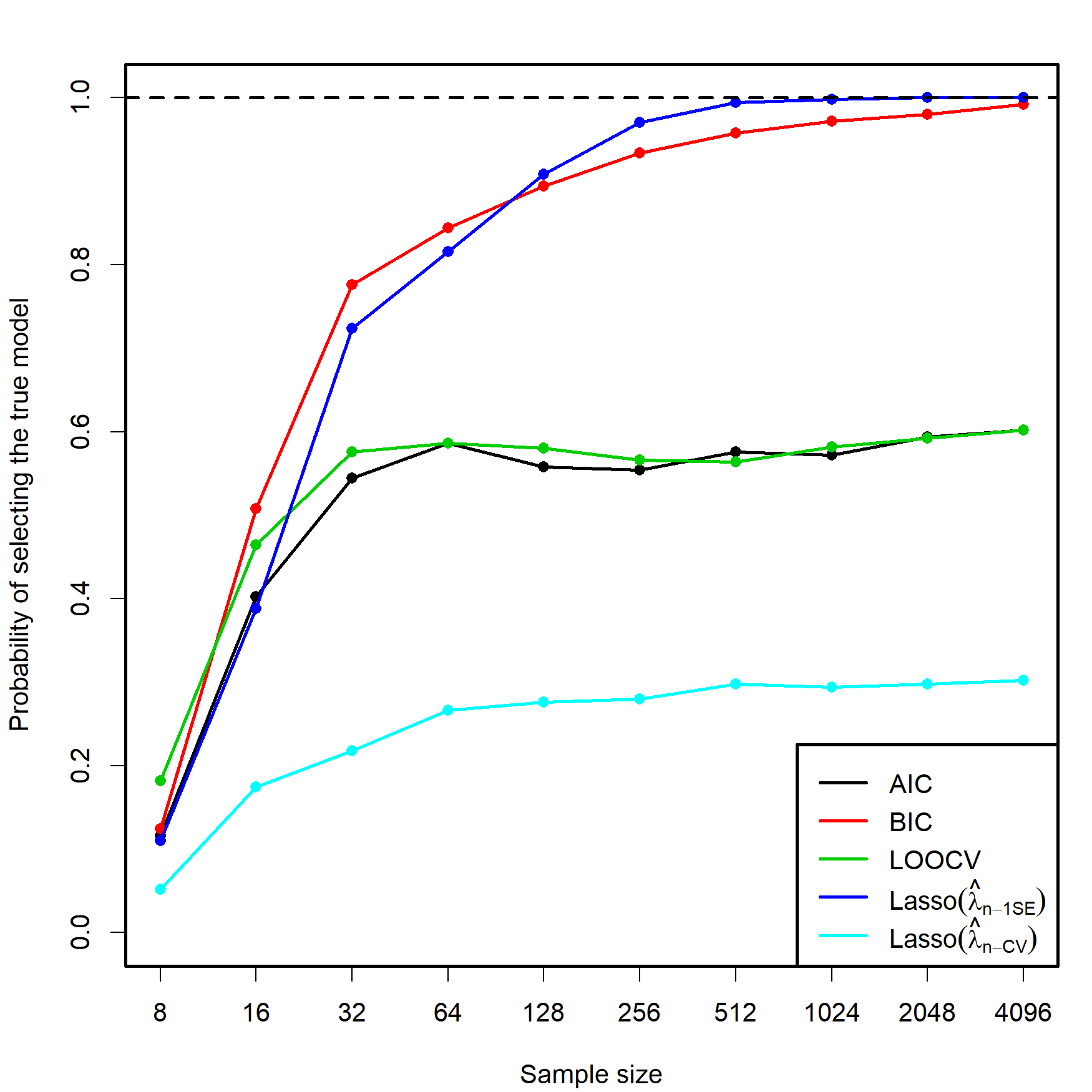
Figure 4.7: Estimation of the probability of selecting the correct model by lasso selection based on \(\hat{\lambda}_{n\text{-CV}}\) and \(\hat\lambda_{n\text{-1SE}},\) and by minimizing the AIC, BIC, and LOOCV criteria in an exhaustive search (see Figure 3.5). There are \(p=5\) independent predictors and the correct model contained two predictors. The probability was estimated with \(M=500\) Monte Carlo runs.
In addition to the insights from Figure 3.5, Figure 4.7 shows interesting results, described next. Recall that the simulation study was performed with independent predictors.
- Lasso-selection based on \(\hat{\lambda}_{n\text{-CV}}\) is inconsistent. It tends to select more predictors than required, as AIC does, yet its performance is much worse (about a \(0.25\) probability of recovering the true model!). This result is somehow coherent with what would be expected from Shao (1993)’s result on the inconsistency of LOOCV.
- Lasso-selection based on \(\hat\lambda_{n\text{-1SE}}\) seems to be129 consistent and imitates the performance of the BIC.130 Observe that the overpenalization given by the one standard error rule somehow resembles the overpenalization of BIC with respect to AIC.
Exercise 4.2 Implement the lasso part of the simulation study behind Figure 4.7:
- Sample from (3.4).
- Compute the \(\hat{\lambda}_{n\text{-CV}}\) and \(\hat\lambda_{n\text{-1SE}}.\)
- Identify the estimated coefficients for \(\hat{\lambda}_{n\text{-CV}}\) and \(\hat\lambda_{n\text{-1SE}}\) that are different from zero.
- Repeat Steps 1–3 \(M=200\) times. Estimate by Monte Carlo the probability of selecting the true model.
- Move \(n=2^\ell,\) \(\ell=3,\ldots,12.\)
Once you have a working solution, increase \(M\) to approach the settings in Figure 4.7 (or go beyond!). You can increase also \(p\) and pad \(\boldsymbol{\beta}\) with zeros.
Exercise 4.3 Investigate what happens if Step 2 of the previous exercise is replaced by the computation of \(\hat{\lambda}_{k\text{-CV}}\) and \(\hat\lambda_{k\text{-1SE}},\) where:
- \(k=2.\)
- \(k=4.\)
- \(k=8.\)
- \(k=16.\)
Take \(\ell=3,\ldots,12\) and overlay the eight curves together.
Exercise 4.4 Investigate what happens if Step 2 of the previous exercise is replaced by the computation of \(\hat{\lambda}_{k\text{-CV}}\) and \(\hat\lambda_{k\text{-1SE}},\) where:
- \(k=n/8.\)
- \(k=n/4.\)
- \(k=n/2.\)
- \(k=n.\)
Take \(\ell=3,\ldots,12\) and overlay the eight curves together.
Exercise 4.5 Investigate what happens if Step 1 is replaced by sampling from dependent predictors. Particularly, sample from (3.4) but with \((X_1,\ldots,X_5)^\top\sim\mathcal{N}_5(\mathbf{0},\boldsymbol\Sigma),\) with \(\boldsymbol\Sigma=(\sigma_{ij})\) such that:
-
\(\sigma_{ij}=\rho^{|i-j|}\) for \(i,j=1,\ldots,5\) and \(\rho=0.25,0.50,0.99.\) Hint: use the
toeplitzfunction. - \(\sigma_{ij}=\frac{c}{2q-1}\) and \(\sigma_{ii}=1,\) for \(i,j=1,\ldots,5,\) \(i\neq j,\) where \(q=2\) (number of non-zero entries of \(\boldsymbol{\beta}\)). Take \(c=0.75.\)
- Same as b., but with \(c=2.\)
4.2 Constrained linear models
As outlined in the previous section, after doing variable selection with lasso,131 two possibilities are: (i) fit a linear model to the lasso-selected predictors; (ii) run a stepwise selection starting from the lasso-selected model to try to further improve the model.132
Let’s explore the intuitive idea behind (i) in more detail. For the sake of exposition, assume that among \(p\) predictors, lasso zeroed out the first \(q\) of them.133 Then, once \(q\) is known, we would seek to fit the model
\[\begin{align*} Y=\beta_0+\beta_1X_1+\cdots+\beta_pX_p+\varepsilon,\quad \text{subject to} \quad\beta_1=\cdots=\beta_q=0. \end{align*}\]
This is a very simple constraint that we know how to solve: just include the \(p-q\) remaining predictors in the model and fit it. It is however a specific case of a linear constraint on \(\boldsymbol\beta,\) since \(\beta_1=\cdots=\beta_q=0\) is expressible as
\[\begin{align} \begin{pmatrix} \mathbf{I}_q & \mathbf{0}_{q\times (p-q)} \end{pmatrix}_{q\times p}\boldsymbol\beta_{-1}=\mathbf{0}_q,\tag{4.11} \end{align}\]
where \(\mathbf{I}_q\) is an \(q\times q\) identity matrix and \(\boldsymbol\beta_{-1}=(\beta_1,\ldots,\beta_p)^\top.\) The constraint in (4.11) can be generalized as \(\mathbf{A}\boldsymbol{\beta}_{-1}=\mathbf{c},\) which results in the (linearly) constrained linear model
\[\begin{align} Y=\beta_0+\beta_1X_1+\cdots+\beta_pX_p+\varepsilon,\quad \text{subject to}\quad \mathbf{A}\boldsymbol{\beta}_{-1}=\mathbf{c},\tag{4.12} \end{align}\]
where \(\mathbf{A}\) is an \(q\times p\) matrix134 of rank \(q\) and \(\mathbf{c}\in\mathbb{R}^q.\) The constrained linear model (4.12) is useful when there is prior information available about a linear relation that the coefficients of the linear model must satisfy (e.g., in piecewise polynomial fitting).
Before fitting the model (4.12), let’s assume from now on that the variables \(Y\) and \(X_1,\ldots,X_p,\) as well the sample \(\{(\mathbf{X}_i,Y_i)\}_{i=1}^n,\) are centered (see the tip at the end of Section 2.4.4). This means that \(\bar Y=0\) and that \(\bar{\mathbf{X}}:=(\bar X_1,\ldots,\bar X_p)^\top\) is zero. More importantly, it also means that \(\beta_0\) and \(\hat\beta_0\) are null, hence they are not included in the model. That is, that the model
\[\begin{align} Y = \beta_1 X_1 + \cdots + \beta_p X_p + \varepsilon \tag{4.13} \end{align}\]
is considered. In this setting, \(\boldsymbol\beta=(\beta_1,\ldots,\beta_p)^\top\;\)135 and \(\hat{\boldsymbol\beta}=(\mathbb{X}^\top\mathbb{X})^{-1}\mathbb{X}^\top\mathbf{Y}\) is the least squares estimator, with the design matrix \(\mathbb{X}\) now omitting the first column of ones.
Now, the estimator of \(\boldsymbol\beta\) in (4.13) from a sample \(\{(\mathbf{X}_i,Y_i)\}_{i=1}^n\) under the linear constraint \(\mathbf{A}\boldsymbol{\beta}=\mathbf{c}\) is defined as
\[\begin{align} \hat{\boldsymbol{\beta}}_{\mathbf{A}}:=\arg\min_{\substack{\boldsymbol{\beta}\in\mathbb{R}^{p}\\\mathbf{A}\boldsymbol{\beta}=\mathbf{c}}}\text{RSS}_0(\boldsymbol{\beta}),\quad \text{RSS}_0(\boldsymbol{\beta}):=\sum_{i=1}^n(Y_i-\beta_1X_{i1}-\cdots-\beta_p X_{ip})^2.\tag{4.14} \end{align}\]
Solving (4.14) analytically is possible using Lagrange multipliers, and the explicit solution to (4.14) can be seen to be
\[\begin{align} \hat{\boldsymbol\beta}_{\mathbf{A}}=\hat{\boldsymbol\beta}+(\mathbb{X}^\top\mathbb{X})^{-1} \mathbf{A}^\top[\mathbf{A} (\mathbb{X}^\top\mathbb{X})^{-1} \mathbf{A}^\top]^{-1} (\mathbf{c}-\mathbf{A}\hat{\boldsymbol\beta}).\tag{4.15} \end{align}\]
For the general case given in (4.12), in which neither \(Y\) and \(\mathbf{X}\) nor the sample are centered, the estimator of \(\boldsymbol\beta\) in (4.12) is unaltered for the slopes and equals (4.15). The intercept is given by \[\begin{align*} \hat{\beta}_{\mathbf{A},0}=\bar Y-\bar{\mathbf{X}}^\top\hat{\boldsymbol{\beta}}_{\mathbf{A}}. \end{align*}\]
The next code illustrates how to fit a linear model with constraints in practice.
# Simulate data
set.seed(123456)
n <- 50
p <- 3
x1 <- rnorm(n, mean = 1)
x2 <- rnorm(n, mean = 2)
x3 <- rnorm(n, mean = 3)
eps <- rnorm(n, sd = 0.5)
y <- 1 + 2 * x1 - 3 * x2 + x3 + eps

# Center the data and compute design matrix
x1_cen <- x1 - mean(x1)
x2_cen <- x2 - mean(x2)
x3_cen <- x3 - mean(x3)
y_cen <- y - mean(y)
X <- cbind(x1_cen, x2_cen, x3_cen)

# Linear restriction: use that
# beta_1 + beta_2 + beta_3 = 0
# beta_2 = -3
# In this case q = 2. The restriction is codified as
A <- rbind(c(1, 1, 1),
           c(0, 1, 0))
c <- c(0, -3)

# Fit model without intercept
S <- solve(crossprod(X))
beta_hat <- S %*% t(X) %*% y_cen
beta_hat
##              [,1]
## x1_cen  1.9873776
## x2_cen -3.1449015
## x3_cen  0.9828062

# Restricted fit enforcing A * beta = c
beta_hat_A <- beta_hat +
  S %*% t(A) %*% solve(A %*% S %*% t(A)) %*% (c - A %*% beta_hat)
beta_hat_A
##              [,1]
## x1_cen  2.0154729
## x2_cen -3.0000000
## x3_cen  0.9845271

# Intercept of the constrained fit
beta_hat_A_0 <- mean(y) - c(mean(x1), mean(x2), mean(x3)) %*% beta_hat_A
beta_hat_A_0
##         [,1]
## [1,] 1.02824
What about inference? In principle, it can be obtained analogously to how the inference for the unconstrained linear model was obtained in Section 2.4, since the distribution of \(\hat{\boldsymbol\beta}_{\mathbf{A}}\) under the assumptions of the linear model is straightforward to obtain. We keep assuming that the model is centered. Then, recall that (4.15) can be expressed as
\[\begin{align*} \hat{\boldsymbol\beta}_{\mathbf{A}}=&\,(\mathbb{X}^\top\mathbb{X})^{-1} \mathbf{A}^\top[\mathbf{A} (\mathbb{X}^\top\mathbb{X})^{-1} \mathbf{A}^\top]^{-1}\mathbf{c}\\ &+\left(\mathbf{I}_p-(\mathbb{X}^\top\mathbb{X})^{-1} \mathbf{A}^\top[\mathbf{A} (\mathbb{X}^\top\mathbb{X})^{-1} \mathbf{A}^\top]^{-1} \mathbf{A}\right)\hat{\boldsymbol\beta}. \end{align*}\]
Therefore, using (1.4) and proceeding similarly to (2.11),
\[\begin{align} \hat{\boldsymbol\beta}_{\mathbf{A}}\sim\mathcal{N}_p\left(\boldsymbol{\beta}+b(\boldsymbol{\beta}, \mathbf{A}, \mathbf{c}, \mathbb{X}),\sigma^2(\mathbb{X}^\top\mathbb{X})^{-1}-v(\sigma^2,\mathbf{A},\mathbb{X})\right),\tag{4.16} \end{align}\]
where
\[\begin{align*} b(\boldsymbol{\beta}, \mathbf{A}, \mathbf{c}, \mathbb{X})&:=(\mathbb{X}^\top\mathbb{X})^{-1} \mathbf{A}^\top[\mathbf{A} (\mathbb{X}^\top\mathbb{X})^{-1} \mathbf{A}^\top]^{-1}(\mathbf{c}- \mathbf{A}\boldsymbol{\beta}),\\ v(\sigma^2,\mathbf{A},\mathbb{X})&:=\sigma^2(\mathbb{X}^\top\mathbb{X})^{-1}\mathbf{A}^\top[\mathbf{A} (\mathbb{X}^\top\mathbb{X})^{-1} \mathbf{A}^\top]^{-1}\mathbf{A}(\mathbb{X}^\top\mathbb{X})^{-1}. \end{align*}\]
The inference for constrained linear models is not built within base R. Therefore, we just give a couple of insights about (4.16) and do not pursue inference further. Note that:
The variances of \(\hat{\beta}_{\mathbf{A},j},\) \(j=1,\ldots, p,\) decrease with respect to the variances of \(\hat{\beta}_j,\) given by the diagonal elements of \(\sigma^2(\mathbb{X}^\top\mathbb{X})^{-1}.\) This is perfectly coherent, after all we are constraining the possible values that the estimator of \(\boldsymbol\beta\) can take in order to accommodate \(\mathbf{A}\boldsymbol{\beta}=\mathbf{c}.\) More importantly, these variances remain the same irrespective of whether \(\mathbf{A}\boldsymbol{\beta}=\mathbf{c}\) holds or not.136
The bias of \(\hat{\boldsymbol\beta}_{\mathbf{A}}\) depends on the veracity of \(\mathbf{A}\boldsymbol{\beta}=\mathbf{c}\). If the restriction is verified, then \(b(\boldsymbol{\beta}, \mathbf{A}, \mathbf{c}, \mathbb{X})=\mathbf{0}\) and \(\hat{\boldsymbol\beta}_{\mathbf{A}}\) is still unbiased. However, if \(\mathbf{A}\boldsymbol{\beta}\neq\mathbf{c},\) then \(\hat{\boldsymbol\beta}_{\mathbf{A}}\) is severely biased in estimating \(\boldsymbol\beta.\)
Exercise 4.6 Verify by Monte Carlo that the covariance matrix in (4.16) is correct. To do so:
- Choose \(\boldsymbol\beta,\) \(\mathbf{A},\) and \(\mathbf{c}\) at your convenience.
- Sample \(n=50\) observations for the predictors.
- Sample \(n=50\) observations for the responses from a linear model based on \(\boldsymbol\beta.\) Use the same \(n\) observations for the predictors from Step 2.
- Compute \(\hat{\boldsymbol\beta}_{\mathbf{A}}.\)
- Repeat Steps 3–4 \(M=500\) times, saving each time \(\hat{\boldsymbol\beta}_{\mathbf{A}}.\)
- Compute the sample covariance matrix of the \(\hat{\boldsymbol\beta}_{\mathbf{A}}\)’s.
- Compare it with the covariance matrix in (4.16).
Exercise 4.7 Do the same study for checking the expectation in (4.16), for the cases in which \(\mathbf{A}\boldsymbol{\beta}=\mathbf{c}\) and \(\mathbf{A}\boldsymbol{\beta}\neq\mathbf{c}.\)
4.3 Multivariate multiple linear model
So far, we have been interested in predicting/explaining a single response \(Y\) from a set of predictors \(X_1,\ldots,X_p.\) However, we might want to predict/explain several responses \(Y_1,\ldots,Y_q.\)137 As we will see, the model construction and estimation are quite analogous to the univariate multiple linear model, yet more cumbersome in notation.
4.3.1 Model formulation and least squares
The centered138 population version of the multivariate multiple linear model is
\[\begin{align*} Y_1&=\beta_{11}X_1+\cdots+\beta_{p1}X_p+\varepsilon_1, \\ & \vdots\\ Y_q&=\beta_{1q}X_1+\cdots+\beta_{pq}X_p+\varepsilon_q, \end{align*}\]
or, equivalently in matrix form,
\[\begin{align} \mathbf{Y}=\mathbf{B}^\top\mathbf{X}+\boldsymbol{\varepsilon}\tag{4.17} \end{align}\]
where \(\boldsymbol{\varepsilon}:=(\varepsilon_1,\ldots,\varepsilon_q)^\top\) is a random vector with null expectation, \(\mathbf{Y}=(Y_1,\ldots,Y_q)^\top\) and \(\mathbf{X}=(X_1,\ldots,X_p)^\top\) are random vectors, and
\[\begin{align*} \mathbf{B}=\begin{pmatrix} \beta_{11} & \ldots & \beta_{1q} \\ \vdots & \ddots & \vdots \\ \beta_{p1} & \ldots & \beta_{pq} \end{pmatrix}_{p\times q}. \end{align*}\]
Clearly, this construction implies that the conditional expectation of the random vector \(\mathbf{Y}\) is
\[\begin{align*} \mathbb{E}[\mathbf{Y} \mid \mathbf{X}=\mathbf{x}]=\mathbf{B}^\top\mathbf{x}. \end{align*}\]
Given a sample \(\{(\mathbf{X}_i,\mathbf{Y}_i)\}_{i=1}^n\) of observations of \((X_1,\ldots,X_p)\) and \((Y_1,\ldots,Y_q),\) the sample version of (4.17) is
\[\begin{align} \begin{pmatrix} Y_{11} & \ldots & Y_{1q} \\ \vdots & \ddots & \vdots \\ Y_{n1} & \ldots & Y_{nq} \end{pmatrix}_{n\times q}\!\!\! &= \begin{pmatrix} X_{11} & \ldots & X_{1p} \\ \vdots & \ddots & \vdots \\ X_{n1} & \ldots & X_{np} \end{pmatrix}_{n\times p} \begin{pmatrix} \beta_{11} & \ldots & \beta_{1q} \\ \vdots & \ddots & \vdots \\ \beta_{p1} & \ldots & \beta_{pq} \end{pmatrix}_{p\times q}\!\!\! + \begin{pmatrix} \varepsilon_{11} & \ldots & \varepsilon_{1q} \\ \vdots & \ddots & \vdots \\ \varepsilon_{n1} & \ldots & \varepsilon_{nq} \end{pmatrix}_{n\times q},\tag{4.18} \end{align}\]
or, equivalently in matrix form,
\[\begin{align} \mathbb{Y}=\mathbb{X}\mathbf{B}+\mathbf{E},\tag{4.19} \end{align}\]
where \(\mathbb{Y},\) \(\mathbb{X},\) and \(\mathbf{E}\) are clearly identified by comparing (4.19) with (4.18).139
The approach for estimating \(\mathbf{B}\) is really similar to the univariate multiple linear model: minimize the sum of squared distances between the responses \(\mathbf{Y}_1,\ldots,\mathbf{Y}_n\) and their explanations \(\mathbf{B}^\top\mathbf{X}_1,\ldots,\mathbf{B}^\top\mathbf{X}_n.\) These distances are now measured by the \(\|\cdot\|_2\) norm in \(\mathbb{R}^q,\) resulting in
\[\begin{align*} \mathrm{RSS}(\mathbf{B})&:=\sum_{i=1}^n\|\mathbf{Y}_i-\mathbf{B}^\top\mathbf{X}_i\|^2_2\\ &=\sum_{i=1}^n(\mathbf{Y}_i-\mathbf{B}^\top\mathbf{X}_i)^\top(\mathbf{Y}_i-\mathbf{B}^\top\mathbf{X}_i)\\ &=\mathrm{tr}\left((\mathbb{Y}-\mathbb{X}\mathbf{B})^\top(\mathbb{Y}-\mathbb{X}\mathbf{B})\right). \end{align*}\]
The similarities with (2.6) are clear and it is immediate to see that (2.6) appears as a special case140 for \(q=1.\) The minimizer of \(\mathrm{RSS}(\mathbf{B})\) is obtained analogously to how the least squares estimator was obtained when \(q=1\):
\[\begin{align} \hat{\mathbf{B}}&:=\arg\min_{\mathbf{B}\in\mathcal{M}_{p\times q}}\mathrm{RSS}(\mathbf{B})=(\mathbb{X}^\top\mathbb{X})^{-1}\mathbb{X}^\top\mathbb{Y}.\tag{4.20} \end{align}\]
Recall that if the responses and predictors are not centered, then the estimate of the intercept is simply obtained from the sample means \(\bar{\mathbf{Y}}:=(\bar Y_1,\ldots,\bar Y_q)^\top\) and \(\bar{\mathbf{X}}=(\bar X_1,\ldots,\bar X_p)^\top\):
\[\begin{align*} \hat{\boldsymbol{\beta}}_0=\bar{\mathbf{Y}}-\hat{\mathbf{B}}^\top\bar{\mathbf{X}}. \end{align*}\]
Equation (4.20) reveals that fitting a \(q\)-multivariate linear model amounts to fitting \(q\) univariate linear models separately! Indeed, recall that \(\mathbf{B}=(\boldsymbol{\beta}_1 \cdots \boldsymbol{\beta}_q),\) where the column vector \(\boldsymbol{\beta}_j\) represents the vector of coefficients of the \(j\)-th univariate linear model. Then, comparing (4.20) with (2.7) (where \(\mathbb{Y}\) consisted of a single column) and by block matrix multiplication, we can clearly see that \(\hat{\mathbf{B}}\) is just the concatenation of the columns of \(\hat{\boldsymbol{\beta}}_j,\) \(j=1,\ldots,q,\) i.e., \(\hat{\mathbf{B}}=(\hat{\boldsymbol{\beta}}_1 \cdots \hat{\boldsymbol{\beta}}_q).\)
As happened in the univariate linear model, if \(p>n\) then the inverse of \(\mathbb{X}^\top\mathbb{X}\) in (4.20) does not exist. In that case, one should either remove predictors or resort to a shrinkage method that avoids inverting \(\mathbb{X}^\top\mathbb{X}.\) It is interesting to note, though, that \(q\) has no effect on the feasibility of the fitting, only \(p\) does. In particular it is possible to compute (4.20) with \(q\gg n,\) and hence \(pq\gg n,\) i.e., the number of estimated parameters can be much larger than \(n\).
We see next how to do multivariate multiple linear regression in R with a simulated example.
# Dimensions and sample size
p <- 3
q <- 2
n <- 100

# A quick way of creating a non-diagonal (valid) covariance matrix for the
# errors
Sigma <- 3 * toeplitz(seq(1, 0.1, l = q))
set.seed(12345)
X <- mvtnorm::rmvnorm(n = n, mean = 1:p, sigma = diag(0.5, nrow = p, ncol = p))
E <- mvtnorm::rmvnorm(n = n, mean = rep(0, q), sigma = Sigma)

# Linear model
B <- matrix((-1)^(1:p) * (1:p), nrow = p, ncol = q, byrow = TRUE)
Y <- X %*% B + E

# Fitting the model (note: Y and X are matrices!)
mod <- lm(Y ~ X)
mod
##
## Call:
## lm(formula = Y ~ X)
##
## Coefficients:
##              [,1]      [,2]
## (Intercept)   0.05017  -0.36899
## X1           -0.54770   2.06905
## X2           -3.01547  -0.78308
## X3            1.88327  -3.00840
# Note that the intercept is markedly different from zero -- that is because
# X is not centered

# Compare with B
B
##      [,1] [,2]
## [1,]   -1    2
## [2,]   -3   -1
## [3,]    2   -3

# Summary of the model: gives q separate summaries, one for each fitted
# univariate model
summary(mod)
## Response Y1 :
##
## Call:
## lm(formula = Y1 ~ X)
##
## Residuals:
##     Min      1Q  Median      3Q     Max
## -4.0432 -1.3513  0.2592  1.1325  3.5298
##
## Coefficients:
##             Estimate Std. Error t value Pr(>|t|)
## (Intercept)  0.05017    0.96251   0.052   0.9585
## X1          -0.54770    0.24034  -2.279   0.0249 *
## X2          -3.01547    0.26146 -11.533  < 2e-16 ***
## X3           1.88327    0.21537   8.745 7.38e-14 ***
## ---
## Signif. codes:  0 '***' 0.001 '**' 0.01 '*' 0.05 '.' 0.1 ' ' 1
##
## Residual standard error: 1.695 on 96 degrees of freedom
## Multiple R-squared:  0.7033, Adjusted R-squared:  0.694
## F-statistic: 75.85 on 3 and 96 DF,  p-value: < 2.2e-16
##
##
## Response Y2 :
##
## Call:
## lm(formula = Y2 ~ X)
##
## Residuals:
##     Min      1Q  Median      3Q     Max
## -4.1385 -0.7922 -0.0486  0.8987  3.6599
##
## Coefficients:
##             Estimate Std. Error t value Pr(>|t|)
## (Intercept)  -0.3690     0.8897  -0.415  0.67926
## X1            2.0691     0.2222   9.314 4.44e-15 ***
## X2           -0.7831     0.2417  -3.240  0.00164 **
## X3           -3.0084     0.1991 -15.112  < 2e-16 ***
## ---
## Signif. codes:  0 '***' 0.001 '**' 0.01 '*' 0.05 '.' 0.1 ' ' 1
##
## Residual standard error: 1.567 on 96 degrees of freedom
## Multiple R-squared:  0.7868, Adjusted R-squared:  0.7801
## F-statistic: 118.1 on 3 and 96 DF,  p-value: < 2.2e-16

# Exactly equivalent to
summary(lm(Y[, 1] ~ X))
##
## Call:
## lm(formula = Y[, 1] ~ X)
##
## Residuals:
##     Min      1Q  Median      3Q     Max
## -4.0432 -1.3513  0.2592  1.1325  3.5298
##
## Coefficients:
##             Estimate Std. Error t value Pr(>|t|)
## (Intercept)  0.05017    0.96251   0.052   0.9585
## X1          -0.54770    0.24034  -2.279   0.0249 *
## X2          -3.01547    0.26146 -11.533  < 2e-16 ***
## X3           1.88327    0.21537   8.745 7.38e-14 ***
## ---
## Signif. codes:  0 '***' 0.001 '**' 0.01 '*' 0.05 '.' 0.1 ' ' 1
##
## Residual standard error: 1.695 on 96 degrees of freedom
## Multiple R-squared:  0.7033, Adjusted R-squared:  0.694
## F-statistic: 75.85 on 3 and 96 DF,  p-value: < 2.2e-16
summary(lm(Y[, 2] ~ X))
##
## Call:
## lm(formula = Y[, 2] ~ X)
##
## Residuals:
##     Min      1Q  Median      3Q     Max
## -4.1385 -0.7922 -0.0486  0.8987  3.6599
##
## Coefficients:
##             Estimate Std. Error t value Pr(>|t|)
## (Intercept)  -0.3690     0.8897  -0.415  0.67926
## X1            2.0691     0.2222   9.314 4.44e-15 ***
## X2           -0.7831     0.2417  -3.240  0.00164 **
## X3           -3.0084     0.1991 -15.112  < 2e-16 ***
## ---
## Signif. codes:  0 '***' 0.001 '**' 0.01 '*' 0.05 '.' 0.1 ' ' 1
##
## Residual standard error: 1.567 on 96 degrees of freedom
## Multiple R-squared:  0.7868, Adjusted R-squared:  0.7801
## F-statistic: 118.1 on 3 and 96 DF,  p-value: < 2.2e-16
Let’s see another quick example using the iris dataset.
# When we want to add several variables of a dataset as responses through a
# formula interface, we have to use cbind() in the response. Doing
# "Petal.Width + Petal.Length ~ ..." is INCORRECT, as lm will understand
# "I(Petal.Width + Petal.Length) ~ ..." and do one single regression

# Predict Petal's measurements from Sepal's
mod_iris <- lm(cbind(Petal.Width, Petal.Length) ~
                Sepal.Length + Sepal.Width + Species, data = iris)
summary(mod_iris)
## Response Petal.Width :
##
## Call:
## lm(formula = Petal.Width ~ Sepal.Length + Sepal.Width + Species,
##     data = iris)
##
## Residuals:
##      Min       1Q   Median       3Q      Max
## -0.50805 -0.10042 -0.01221  0.11416  0.46455
##
## Coefficients:
##                   Estimate Std. Error t value Pr(>|t|)
## (Intercept)       -0.86897    0.16985  -5.116 9.73e-07 ***
## Sepal.Length       0.06360    0.03395   1.873    0.063 .
## Sepal.Width        0.23237    0.05145   4.516 1.29e-05 ***
## Speciesversicolor  1.17375    0.06758  17.367  < 2e-16 ***
## Speciesvirginica   1.78487    0.07779  22.944  < 2e-16 ***
## ---
## Signif. codes:  0 '***' 0.001 '**' 0.01 '*' 0.05 '.' 0.1 ' ' 1
##
## Residual standard error: 0.1797 on 145 degrees of freedom
## Multiple R-squared:  0.9459, Adjusted R-squared:  0.9444
## F-statistic: 634.3 on 4 and 145 DF,  p-value: < 2.2e-16
##
##
## Response Petal.Length :
##
## Call:
## lm(formula = Petal.Length ~ Sepal.Length + Sepal.Width + Species,
##     data = iris)
##
## Residuals:
##      Min       1Q   Median       3Q      Max
## -0.75196 -0.18755  0.00432  0.16965  0.79580
##
## Coefficients:
##                   Estimate Std. Error t value Pr(>|t|)
## (Intercept)       -1.63430    0.26783  -6.102 9.08e-09 ***
## Sepal.Length       0.64631    0.05353  12.073  < 2e-16 ***
## Sepal.Width       -0.04058    0.08113  -0.500    0.618
## Speciesversicolor  2.17023    0.10657  20.364  < 2e-16 ***
## Speciesvirginica   3.04911    0.12267  24.857  < 2e-16 ***
## ---
## Signif. codes:  0 '***' 0.001 '**' 0.01 '*' 0.05 '.' 0.1 ' ' 1
##
## Residual standard error: 0.2833 on 145 degrees of freedom
## Multiple R-squared:  0.9749, Adjusted R-squared:  0.9742
## F-statistic:  1410 on 4 and 145 DF,  p-value: < 2.2e-16

# The fitted values and residuals are now matrices
head(mod_iris$fitted.values)
##   Petal.Width Petal.Length
## 1   0.2687095     1.519831
## 2   0.1398033     1.410862
## 3   0.1735565     1.273483
## 4   0.1439590     1.212910
## 5   0.2855861     1.451142
## 6   0.3807391     1.697490
head(mod_iris$residuals)
##   Petal.Width Petal.Length
## 1 -0.06870951 -0.119831001
## 2  0.06019672 -0.010861533
## 3  0.02644348  0.026517420
## 4  0.05604099  0.287089900
## 5 -0.08558613 -0.051141525
## 6  0.01926089  0.002510054

# The individual models
mod_iris1 <- lm(Petal.Width ~ Sepal.Length + Sepal.Width + Species, data = iris)
mod_iris2 <- lm(Petal.Length ~ Sepal.Length + Sepal.Width + Species, data = iris)
summary(mod_iris1)
##
## Call:
## lm(formula = Petal.Width ~ Sepal.Length + Sepal.Width + Species,
##     data = iris)
##
## Residuals:
##      Min       1Q   Median       3Q      Max
## -0.50805 -0.10042 -0.01221  0.11416  0.46455
##
## Coefficients:
##                   Estimate Std. Error t value Pr(>|t|)
## (Intercept)       -0.86897    0.16985  -5.116 9.73e-07 ***
## Sepal.Length       0.06360    0.03395   1.873    0.063 .
## Sepal.Width        0.23237    0.05145   4.516 1.29e-05 ***
## Speciesversicolor  1.17375    0.06758  17.367  < 2e-16 ***
## Speciesvirginica   1.78487    0.07779  22.944  < 2e-16 ***
## ---
## Signif. codes:  0 '***' 0.001 '**' 0.01 '*' 0.05 '.' 0.1 ' ' 1
##
## Residual standard error: 0.1797 on 145 degrees of freedom
## Multiple R-squared:  0.9459, Adjusted R-squared:  0.9444
## F-statistic: 634.3 on 4 and 145 DF,  p-value: < 2.2e-16
summary(mod_iris2)
##
## Call:
## lm(formula = Petal.Length ~ Sepal.Length + Sepal.Width + Species,
##     data = iris)
##
## Residuals:
##      Min       1Q   Median       3Q      Max
## -0.75196 -0.18755  0.00432  0.16965  0.79580
##
## Coefficients:
##                   Estimate Std. Error t value Pr(>|t|)
## (Intercept)       -1.63430    0.26783  -6.102 9.08e-09 ***
## Sepal.Length       0.64631    0.05353  12.073  < 2e-16 ***
## Sepal.Width       -0.04058    0.08113  -0.500    0.618
## Speciesversicolor  2.17023    0.10657  20.364  < 2e-16 ***
## Speciesvirginica   3.04911    0.12267  24.857  < 2e-16 ***
## ---
## Signif. codes:  0 '***' 0.001 '**' 0.01 '*' 0.05 '.' 0.1 ' ' 1
##
## Residual standard error: 0.2833 on 145 degrees of freedom
## Multiple R-squared:  0.9749, Adjusted R-squared:  0.9742
## F-statistic:  1410 on 4 and 145 DF,  p-value: < 2.2e-16
4.3.2 Assumptions and inference
As deduced from what we have seen so far, fitting a multivariate linear regression is more practical than doing \(q\) separate univariate fits (especially if the number of responses \(q\) is large). However, it is not conceptually different. The discussion becomes more interesting in the inference for the multivariate linear regression, where the dependence between the responses has to be taken into account.
In order to achieve inference, we will require some assumptions, these being natural extensions of the ones seen in Section 2.3:
- Linearity: \(\mathbb{E}[\mathbf{Y} \mid \mathbf{X}=\mathbf{x}]=\mathbf{B}^\top\mathbf{x}.\)
- Homoscedasticity: \(\mathbb{V}\text{ar}[\boldsymbol{\varepsilon} \mid X_1=x_1,\ldots,X_p=x_p]=\boldsymbol{\Sigma}.\)
- Normality: \(\boldsymbol{\varepsilon}\sim\mathcal{N}_q(\mathbf{0},\boldsymbol{\Sigma}).\)
- Independence of the errors: \(\boldsymbol{\varepsilon}_1,\ldots,\boldsymbol{\varepsilon}_n\) are independent (or uncorrelated, \(\mathbb{E}[\boldsymbol{\varepsilon}_i\boldsymbol{\varepsilon}_j^\top]=\mathbf{0},\) \(i\neq j,\) since they are assumed to be normal).
Then, a good one-line summary of the multivariate multiple linear model is (independence is implicit)
\[\begin{align*} \mathbf{Y} \mid \mathbf{X}=\mathbf{x}\sim \mathcal{N}_q(\mathbf{B}^\top\mathbf{x},\boldsymbol{\Sigma}). \end{align*}\]
Based on these assumptions, the key result for rooting inference is the distribution of \(\hat{\mathbf{B}}=(\hat{\boldsymbol{\beta}}_1 \cdots \hat{\boldsymbol{\beta}}_q)\) as an estimator of \(\mathbf{B}=(\boldsymbol{\beta}_1 \cdots \boldsymbol{\beta}_q).\) This result is now more cumbersome,141 but we can state it as
\[\begin{align} \hat{\boldsymbol{\beta}}_j&\sim\mathcal{N}_{p}\left(\boldsymbol{\beta}_j,\sigma_j^2(\mathbb{X}^\top\mathbb{X})^{-1}\right),\quad j=1,\ldots,q,\tag{4.21}\\ \begin{pmatrix} \hat{\boldsymbol{\beta}}_j\\ \hat{\boldsymbol{\beta}}_k \end{pmatrix}&\sim\mathcal{N}_{2p}\left(\begin{pmatrix} \boldsymbol{\beta}_j\\ \boldsymbol{\beta}_k \end{pmatrix}, \begin{pmatrix} \sigma_{j}^2(\mathbb{X}^\top\mathbb{X})^{-1} & \sigma_{jk}(\mathbb{X}^\top\mathbb{X})^{-1} \\ \sigma_{jk}(\mathbb{X}^\top\mathbb{X})^{-1} & \sigma_{k}^2(\mathbb{X}^\top\mathbb{X})^{-1} \end{pmatrix} \right),\quad j,k=1,\ldots,q,\tag{4.22} \end{align}\]
where \(\boldsymbol\Sigma=(\sigma_{ij})\) and \(\sigma_{ii}=\sigma_{i}^2.\)142
The results (4.21)–(4.22) open the way for obtaining hypothesis tests on the joint significance of a predictor in the model (for the \(q\) responses, not just for one), confidence intervals for the coefficients, prediction confidence regions for the conditional expectation and the conditional response, the Multivariate ANOVA (MANOVA) decomposition, multivariate extensions of the \(F\)-test, and others. However, due to the correlation between responses and the multivariate nature of the model, these inferential tools are more complex than in the univariate linear model. Therefore, given the increased complexity, we do not go into more details and refer the interested reader to, e.g., Chapter 8 in Seber (1984). We illustrate with code, though, the most important practical aspects.
# Confidence intervals for the parameters
confint(mod_iris)
##                                       2.5 %     97.5 %
## Petal.Width:(Intercept)        -1.204674903 -0.5332662
## Petal.Width:Sepal.Length       -0.003496659  0.1307056
## Petal.Width:Sepal.Width         0.130680383  0.3340610
## Petal.Width:Speciesversicolor   1.040169583  1.3073259
## Petal.Width:Speciesvirginica    1.631118293  1.9386298
## Petal.Length:(Intercept)       -2.163654566 -1.1049484
## Petal.Length:Sepal.Length       0.540501864  0.7521177
## Petal.Length:Sepal.Width       -0.200934599  0.1197646
## Petal.Length:Speciesversicolor  1.959595164  2.3808588
## Petal.Length:Speciesvirginica   2.806663658  3.2915610
# Warning! Do not confuse Petal.Width:Sepal.Length with an interaction term!
# It is meant to represent the Response:Predictor coefficient

# Prediction -- now more limited without confidence intervals implemented
predict(mod_iris, newdata = iris[1:3, ])
##   Petal.Width Petal.Length
## 1   0.2687095     1.519831
## 2   0.1398033     1.410862
## 3   0.1735565     1.273483

# MANOVA table
manova(mod_iris)
## Call:
##    manova(mod_iris)
##
## Terms:
##                 Sepal.Length Sepal.Width  Species Residuals
## Petal.Width          57.9177      6.3975  17.5745    4.6802
## Petal.Length        352.8662     50.0224  49.7997   11.6371
## Deg. of Freedom            1           1        2       145
##
## Residual standard errors: 0.1796591 0.2832942
## Estimated effects may be unbalanced

# "Same" as the "Sum Sq" and "Df" entries of
anova(mod_iris1)
## Analysis of Variance Table
##
## Response: Petal.Width
##               Df Sum Sq Mean Sq F value    Pr(>F)
## Sepal.Length   1 57.918  57.918 1794.37 < 2.2e-16 ***
## Sepal.Width    1  6.398   6.398  198.21 < 2.2e-16 ***
## Species        2 17.574   8.787  272.24 < 2.2e-16 ***
## Residuals    145  4.680   0.032
## ---
## Signif. codes:  0 '***' 0.001 '**' 0.01 '*' 0.05 '.' 0.1 ' ' 1
anova(mod_iris2)
## Analysis of Variance Table
##
## Response: Petal.Length
##               Df Sum Sq Mean Sq F value    Pr(>F)
## Sepal.Length   1 352.87  352.87 4396.78 < 2.2e-16 ***
## Sepal.Width    1  50.02   50.02  623.29 < 2.2e-16 ***
## Species        2  49.80   24.90  310.26 < 2.2e-16 ***
## Residuals    145  11.64    0.08
## ---
## Signif. codes:  0 '***' 0.001 '**' 0.01 '*' 0.05 '.' 0.1 ' ' 1

# anova() serves for assessing the significance of including a new predictor
# for explaining all the responses. This is based on an extension of the
# *sequential* ANOVA table briefly covered in Section 2.6. The hypothesis test
# is by default conducted with the Pillai statistic (an extension of the F-test)
anova(mod_iris)
## Analysis of Variance Table
##
##               Df  Pillai approx F num Df den Df    Pr(>F)
## (Intercept)    1 0.99463  13332.6      2    144 < 2.2e-16 ***
## Sepal.Length   1 0.97030   2351.9      2    144 < 2.2e-16 ***
## Sepal.Width    1 0.81703    321.5      2    144 < 2.2e-16 ***
## Species        2 0.89573     58.8      4    290 < 2.2e-16 ***
## Residuals    145
## ---
## Signif. codes:  0 '***' 0.001 '**' 0.01 '*' 0.05 '.' 0.1 ' ' 1
4.3.3 Shrinkage
Applying shrinkage is also possible in multivariate linear models. In particular, this allows to fit models with \(p\gg n\) predictors.
The glmnet package implements the elastic net regularization for multivariate linear models. It features extensions of the \(\|\cdot\|_1\) and \(\|\cdot\|_2\) norm penalties for a vector of parameters in \(\mathbb{R}^p,\) as considered in Section 4.1, to norms for a matrix of parameters of size \(p\times q.\) Precisely:
- The ridge penalty \(\|\boldsymbol\beta_{-1}\|_2^2\) extends to \(\|\mathbf{B}\|_{\mathrm{F}}^2,\) where \(\|\mathbf{B}\|_{\mathrm{F}}=\sqrt{\sum_{i=1}^p\sum_{j=1}^q\beta_{ij}^2}\) is the Frobenius norm of \(\mathbf{B}.\) This is a global penalty to shrink \(\mathbf{B}.\)
- The lasso penalty \(\|\boldsymbol\beta_{-1}\|_1\) extends143 to \(\sum_{j=1}^p\|\mathbf{B}_j\|_2,\) where \(\mathbf{B}_j\) is the \(j\)-th row of \(\mathbf{B}.\) This is a rowwise penalty that seeks to effectively remove rows of \(\mathbf{B},\) thus eliminating predictors.144
Taking these two extensions into account, the elastic net loss is defined as:
\[\begin{align} \text{RSS}(\mathbf{B})+\lambda\left(\alpha\sum_{j=1}^p\|\mathbf{B}_j\|_2+(1-\alpha)\|\mathbf{B}\|_{\mathrm{F}}^2\right).\tag{4.23} \end{align}\]
Clearly, ridge regression corresponds to \(\alpha=0\) (quadratic penalty) and lasso to \(\alpha=1\) (rowwise penalty). And if \(\lambda=0,\) we are back to the least squares problem and theory. The optimization of (4.23) gives
\[\begin{align*} \hat{\mathbf{B}}_{\lambda,\alpha}:=\arg\min_{\mathbf{B}\in\mathcal{M}_{p\times q}}\left\{ \text{RSS}(\mathbf{B})+\lambda\left(\alpha\sum_{j=1}^p\|\mathbf{B}_j\|_2+(1-\alpha)\|\mathbf{B}\|_{\mathrm{F}}^2\right)\right\}. \end{align*}\]
From here, the workflow is very similar to the univariate linear model: we have to be aware that a standardization of \(\mathbb{X}\) and \(\mathbb{Y}\) takes place in glmnet; there are explicit formulas for the ridge regression estimator, but not for lasso; tuning parameter selection of \(\lambda\) is done by \(k\)-fold cross-validation and its one standard error variant; variable selection (zeroing of rows in \(\mathbf{B}\)) can be done with lasso.
The following chunk of code illustrates some of these points using glmnet::glmnet with family = "mgaussian" (do not forget this argument!).
# Simulate data
n <- 500
p <- 50
q <- 10
set.seed(123456)
X <- mvtnorm::rmvnorm(n = n, mean = p:1, sigma = 5 * 0.5^toeplitz(1:p))
E <- mvtnorm::rmvnorm(n = n, mean = rep(0, q), sigma = toeplitz(q:1))
B <- 5 * (2 / (0.5 * (1:p - 15)^2 + 2) + 1 / (0.1 * (1:p - 40)^2 + 1)) %*%
  t(1 / sqrt(1:q))
Y <- X %*% B + E

# Visualize B -- dark violet is close to 0
image(1:q, 1:p, t(B), col = viridisLite::viridis(20), xlab = "q", ylab = "p")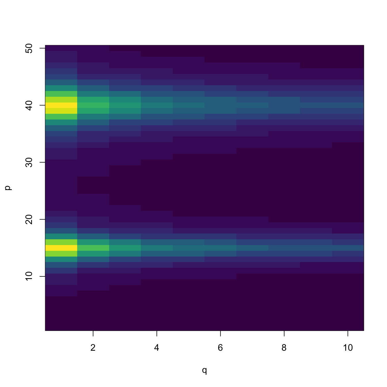
# Lasso path fit
mfit <- glmnet(x = X, y = Y, family = "mgaussian", alpha = 1)

# A list of models for each response
str(mfit$beta, 1)
## List of 10
##  $ y1 :Formal class 'dgCMatrix' [package "Matrix"] with 6 slots
##  $ y2 :Formal class 'dgCMatrix' [package "Matrix"] with 6 slots
##  $ y3 :Formal class 'dgCMatrix' [package "Matrix"] with 6 slots
##  $ y4 :Formal class 'dgCMatrix' [package "Matrix"] with 6 slots
##  $ y5 :Formal class 'dgCMatrix' [package "Matrix"] with 6 slots
##  $ y6 :Formal class 'dgCMatrix' [package "Matrix"] with 6 slots
##  $ y7 :Formal class 'dgCMatrix' [package "Matrix"] with 6 slots
##  $ y8 :Formal class 'dgCMatrix' [package "Matrix"] with 6 slots
##  $ y9 :Formal class 'dgCMatrix' [package "Matrix"] with 6 slots
##  $ y10:Formal class 'dgCMatrix' [package "Matrix"] with 6 slots

# Tuning parameter selection by 10-fold cross-validation
set.seed(12345)
kcv_lasso_m <- cv.glmnet(x = X, y = Y, family = "mgaussian", alpha = 1)
kcv_lasso_m$lambda.min
## [1] 0.135243
kcv_lasso_m$lambda.1se
## [1] 0.497475

# Location of both optimal lambdas in the CV loss function
ind_min <- which.min(kcv_lasso_m$cvm)
plot(kcv_lasso_m)
abline(h = kcv_lasso_m$cvm[ind_min] + c(0, kcv_lasso_m$cvsd[ind_min]))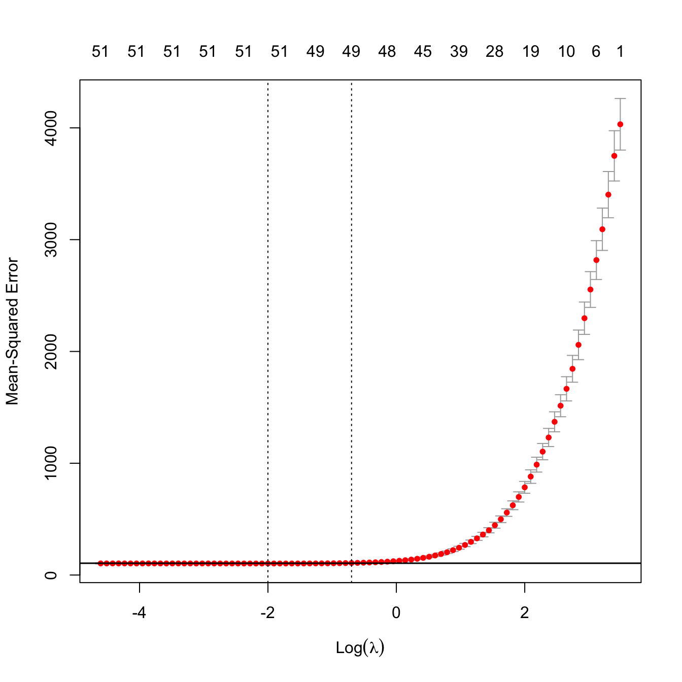
# Extract the coefficients associated with some fits
coefs <- coef(kcv_lasso_m, s = c(kcv_lasso_m$lambda.min, kcv_lasso_m$lambda.1se))
str(coefs, 1)
## List of 10
##  $ y1 :Formal class 'dgCMatrix' [package "Matrix"] with 6 slots
##  $ y2 :Formal class 'dgCMatrix' [package "Matrix"] with 6 slots
##  $ y3 :Formal class 'dgCMatrix' [package "Matrix"] with 6 slots
##  $ y4 :Formal class 'dgCMatrix' [package "Matrix"] with 6 slots
##  $ y5 :Formal class 'dgCMatrix' [package "Matrix"] with 6 slots
##  $ y6 :Formal class 'dgCMatrix' [package "Matrix"] with 6 slots
##  $ y7 :Formal class 'dgCMatrix' [package "Matrix"] with 6 slots
##  $ y8 :Formal class 'dgCMatrix' [package "Matrix"] with 6 slots
##  $ y9 :Formal class 'dgCMatrix' [package "Matrix"] with 6 slots
##  $ y10:Formal class 'dgCMatrix' [package "Matrix"] with 6 slots

# Predictions for the first two observations
preds <- predict(kcv_lasso_m, type = "response",
                 s = c(kcv_lasso_m$lambda.min, kcv_lasso_m$lambda.1se),
                 newx = X[1:2, ])
preds
## , , s=0.135243
##
##            y1       y2       y3       y4       y5       y6       y7       y8       y9      y10
## [1,] 1607.532 1137.740 928.9553 804.5352 719.4861 656.1383 607.9023 568.9489 536.3892 508.3132
## [2,] 1598.747 1130.989 923.1741 799.3845 715.3698 652.8120 604.2244 565.1894 531.9679 504.8820
##
## , , s=0.497475
##
##            y1       y2       y3       y4       y5       y6       y7       y8       y9      y10
## [1,] 1606.685 1137.092 928.4553 804.0957 719.0616 655.7909 607.5870 568.5401 536.0135 508.0311
## [2,] 1600.321 1132.040 924.0621 800.1538 715.9371 653.3917 604.7983 565.6777 532.6244 505.4317
Finally, the next animation helps visualizing how the zeroing of the lasso happens for the estimator of \(\mathbf{B}\) with overall low absolute values on the previous simulated model.
manipulate::manipulate({

  # Color
  col <- viridisLite::viridis(20)

  # Common zlim
  zlim <- range(B) + c(-0.25, 0.25)

  # Plot true B
  par(mfrow = c(1, 2))
  image(1:q, 1:p, t(B), col = col, xlab = "q", ylab = "p", zlim = zlim,
        main = "B")

  # Extract B_hat from the lasso fit, a p x q matrix
  B_hat <- sapply(seq_along(mfit$beta), function(i) mfit$beta[i][[1]][, j])

  # Put as black rows the predictors included
  not_zero <- abs(B_hat) > 0
  image(1:q, 1:p, t(not_zero), breaks = c(0.5, 1),
        col = rgb(1, 1, 1, alpha = 0.1), add = TRUE)

  # For B_hat
  image(1:q, 1:p, t(B_hat), col = col, xlab = "q", ylab = "p", zlim = zlim,
        main = "Bhat")
  image(1:q, 1:p, t(not_zero), breaks = c(0.5, 1),
        col = rgb(1, 1, 1, alpha = 0.1), add = TRUE)

}, j = manipulate::slider(min = 1, max = ncol(mfit$beta$y1), step = 1,
                          label = "j in lambda(j)"))
4.4 Big data considerations
The computation of the least squares estimator
\[\begin{align} \hat{\boldsymbol{\beta}}=(\mathbb{X}^\top\mathbb{X})^{-1}\mathbb{X}^\top\mathbf{Y}\tag{4.24} \end{align}\]
involves inverting the \((p+1)\times(p+1)\) matrix \(\mathbb{X}^\top\mathbb{X},\) where \(\mathbb{X}\) is an \(n\times(p+1)\) matrix. The vector to be obtained, \(\hat{\boldsymbol{\beta}},\) is of size \(p+1.\) However, computing it directly from (4.24) requires allocating \(\mathcal{O}(np + p^2)\) elements in memory. When \(n\) is very large, this can be prohibitive. In addition, for convenience of the statistical analysis, R’s lm returns several objects of the same size as \(\mathbb{X}\) and \(\mathbf{Y},\) thus notably increasing the memory usage. For these reasons, alternative approaches for computing \(\hat{\boldsymbol{\beta}}\) with big data are required.
An approach for computing (4.24) in a memory-friendly way is to split the computation of \((\mathbb{X}^\top\mathbb{X})^{-1}\) and \(\mathbb{X}^\top\mathbf{Y}\) by blocks that are storable in memory. A possibility is to update sequentially the estimation of the vector of coefficients. This can be done with the following expression, which relates \(\hat{\boldsymbol{\beta}}\) with \(\hat{\boldsymbol{\beta}}_{-i},\) the vector of estimated coefficients without the \(i\)-th datum:
\[\begin{align} \hat{\boldsymbol{\beta}}=\hat{\boldsymbol{\beta}}_{-i}+(\mathbb{X}^\top\mathbb{X})^{-1}\mathbf{x}_{i}\left(Y_{i}-\mathbf{x}_{i}^\top\hat{\boldsymbol{\beta}}_{-i}\right).\tag{4.25} \end{align}\]
In (4.25) above, \(\mathbf{x}_{i}^\top\) is the \(i\)-th row of the design matrix \(\mathbb{X}.\) The expression follows from the Sherman–Morrison formula for an invertible matrix \(\mathbf{A}\) and a vector \(\mathbf{b},\)
\[\begin{align*} (\mathbf{A}+\mathbf{b}\mathbf{b}^\top)^{-1}=\mathbf{A}^{-1}-\frac{\mathbf{A}^{-1}\mathbf{b}\mathbf{b}^\top\mathbf{A}^{-1}}{1+\mathbf{b}^\top\mathbf{A}^{-1}\mathbf{b}}, \end{align*}\]
and from the equalities
\[\begin{align*} \mathbb{X}^\top\mathbb{X}&=\mathbb{X}_{-i}^\top\mathbb{X}_{-i}+\mathbf{x}_{i}\mathbf{x}^\top_{i},\\ \mathbb{X}^\top\mathbf{Y}&=\mathbb{X}_{-i}^\top\mathbf{Y}_{-i}+\mathbf{x}_{i}Y_i^\top, \end{align*}\]
where \(\mathbb{X}_{-i}\) is the \((n-1)\times (p+1)\) matrix obtained by removing the \(i\)-th row of \(\mathbb{X}.\) In (4.25), using again the Sherman–Morrison formula, we can update \((\mathbb{X}^\top\mathbb{X})^{-1}\) easily from \(\left(\mathbb{X}_{-i}^\top\mathbb{X}_{-i}\right)^{-1}\):
\[\begin{align} (\mathbb{X}^\top\mathbb{X})^{-1}=\left(\mathbb{X}_{-i}^\top\mathbb{X}_{-i}\right)^{-1}-\frac{\left(\mathbb{X}_{-i}^\top\mathbb{X}_{-i}\right)^{-1}\mathbf{x}_{i}\mathbf{x}_{i}^\top\left(\mathbb{X}_{-i}^\top\mathbb{X}_{-i}\right)^{-1}}{1+\mathbf{x}_{i}^\top\left(\mathbb{X}_{-i}^\top\mathbb{X}_{-i}\right)^{-1}\mathbf{x}_{i}}.\tag{4.26} \end{align}\]
This has the advantage of not requiring to compute \(\mathbb{X}^\top\mathbb{X}\) and then to invert it. Instead, we work directly with \(\left(\mathbb{X}_{-i}^\top\mathbb{X}_{-i}\right)^{-1},\) which was already computed and has size \((p + 1)\times(p+1).\)
This idea can be iterated and we can compute \(\hat{\boldsymbol{\beta}}\) by the following iterative procedure:
- Start from a reduced dataset \(\mathbb{X}_\mathrm{old}\equiv \mathbb{X}_{-i}\) and \(\mathbf{Y}_\mathrm{old}\equiv \mathbf{Y}_{-i}\) for which the least squares estimate can be computed. Denote it by \(\hat{\boldsymbol{\beta}}_\mathrm{old}\equiv\hat{\boldsymbol{\beta}}_{-i}.\)
- Add one of the remaining data points to get \(\hat{\boldsymbol{\beta}}_\mathrm{new}\equiv\hat{\boldsymbol{\beta}}\) from (4.25) and (4.26).
- Set \(\hat{\boldsymbol{\beta}}_\mathrm{new}\gets\hat{\boldsymbol{\beta}}_\mathrm{old}\) and \(\mathbb{X}_\mathrm{new}\gets\mathbb{X}_\mathrm{old}.\)
- Repeat Steps 2–3 until there are no remaining data points left.
- Return \(\hat{\boldsymbol{\beta}}\gets\hat{\boldsymbol{\beta}}_\mathrm{new}.\)
The main advantage of this iterative procedure is clear: we do not need to store any vector or matrix with \(n\) in the dimension – only matrices of size \(p.\) As a consequence, we do not need to store the data in memory.
A similar iterative approach (yet more sophisticated) is followed by the biglm package. We omit the details here (see Miller (1992)) and just comment the main idea: for computing (4.24), biglm::biglm performs a QR decomposition145 of \(\mathbb{X}\) that is computed iteratively. Then, instead of computing (4.24), it solves the triangular system
\[\begin{align*} \mathbf{R}\hat{\boldsymbol{\beta}}=\mathbf{Q}^\top\mathbf{Y}. \end{align*}\]
Let’s see how biglm::biglm works in practice.
# Not really "big data", but for the sake of illustration
set.seed(12345)
n <- 1e6
p <- 10
beta <- seq(-1, 1, length.out = p)^5
x1 <- matrix(rnorm(n * p), nrow = n, ncol = p)
x1[, p] <- 2 * x1[, 1] + rnorm(n, sd = 0.1) # Add some dependence to predictors
x1[, p - 1] <- 2 - x1[, 2] + rnorm(n, sd = 0.5)
y1 <- 1 + x1 %*% beta + rnorm(n)
x2 <- matrix(rnorm(100 * p), nrow = 100, ncol = p)
y2 <- 1 + x2 %*% beta + rnorm(100)
big_data1 <- data.frame("resp" = y1, "pred" = x1)
big_data2 <- data.frame("resp" = y2, "pred" = x2)

# biglm has a very similar syntax to lm -- but the formula interface does not
# work always as expected
# biglm::biglm(formula = resp ~ ., data = bigData1) # Does not work
# biglm::biglm(formula = y ~ x) # Does not work
# biglm::biglm(formula = resp ~ pred.1 + pred.2, data = bigData1) # Does work,
# but not very convenient for a large number of predictors
# Hack for automatic inclusion of all the predictors
f <- formula(paste("resp ~", paste(names(big_data1)[-1], collapse = " + ")))
biglm_mod <- biglm::biglm(formula = f, data = big_data1)

# lm's call
lm_mod <- lm(formula = resp ~ ., data = big_data1)

# The reduction in size of the resulting object is more than notable
print(object.size(biglm_mod), units = "KB")
## 13.1 Kb
print(object.size(lm_mod), units = "MB")
## 381.5 Mb

# Summaries
s1 <- summary(biglm_mod)
s2 <- summary(lm_mod)
s1
## Large data regression model: biglm::biglm(formula = f, data = big_data1)
## Sample size =  1000000
##                Coef    (95%     CI)     SE      p
## (Intercept)  1.0021  0.9939  1.0104 0.0041 0.0000
## pred.1      -0.9733 -1.0133 -0.9333 0.0200 0.0000
## pred.2      -0.2866 -0.2911 -0.2822 0.0022 0.0000
## pred.3      -0.0535 -0.0555 -0.0515 0.0010 0.0000
## pred.4      -0.0041 -0.0061 -0.0021 0.0010 0.0000
## pred.5      -0.0002 -0.0022  0.0018 0.0010 0.8373
## pred.6       0.0003 -0.0017  0.0023 0.0010 0.7771
## pred.7       0.0026  0.0006  0.0046 0.0010 0.0091
## pred.8       0.0521  0.0501  0.0541 0.0010 0.0000
## pred.9       0.2840  0.2800  0.2880 0.0020 0.0000
## pred.10      0.9867  0.9667  1.0067 0.0100 0.0000
s2
##
## Call:
## lm(formula = resp ~ ., data = big_data1)
##
## Residuals:
##     Min      1Q  Median      3Q     Max
## -4.8798 -0.6735 -0.0013  0.6735  4.9060
##
## Coefficients:
##               Estimate Std. Error  t value Pr(>|t|)
## (Intercept)  1.0021454  0.0041200  243.236  < 2e-16 ***
## pred.1      -0.9732675  0.0199989  -48.666  < 2e-16 ***
## pred.2      -0.2866314  0.0022354 -128.227  < 2e-16 ***
## pred.3      -0.0534834  0.0009997  -53.500  < 2e-16 ***
## pred.4      -0.0040772  0.0009984   -4.084 4.43e-05 ***
## pred.5      -0.0002051  0.0009990   -0.205  0.83731
## pred.6       0.0002828  0.0009989    0.283  0.77706
## pred.7       0.0026085  0.0009996    2.610  0.00907 **
## pred.8       0.0520744  0.0009994   52.105  < 2e-16 ***
## pred.9       0.2840358  0.0019992  142.076  < 2e-16 ***
## pred.10      0.9866851  0.0099876   98.791  < 2e-16 ***
## ---
## Signif. codes:  0 '***' 0.001 '**' 0.01 '*' 0.05 '.' 0.1 ' ' 1
##
## Residual standard error: 0.9993 on 999989 degrees of freedom
## Multiple R-squared:  0.5777, Adjusted R-squared:  0.5777
## F-statistic: 1.368e+05 on 10 and 999989 DF,  p-value: < 2.2e-16

# Further information
s1$mat # Coefficients and their inferences
##                      Coef          (95%          CI)           SE            p
## (Intercept)  1.0021454430  0.9939053491  1.010385537 0.0041200470 0.000000e+00
## pred.1      -0.9732674585 -1.0132653005 -0.933269616 0.0199989210 0.000000e+00
## pred.2      -0.2866314070 -0.2911021089 -0.282160705 0.0022353509 0.000000e+00
## pred.3      -0.0534833941 -0.0554827653 -0.051484023 0.0009996856 0.000000e+00
## pred.4      -0.0040771777 -0.0060739907 -0.002080365 0.0009984065 4.432709e-05
## pred.5      -0.0002051218 -0.0022030377  0.001792794 0.0009989579 8.373098e-01
## pred.6       0.0002828388 -0.0017149118  0.002280589 0.0009988753 7.770563e-01
## pred.7       0.0026085425  0.0006093153  0.004607770 0.0009996136 9.066118e-03
## pred.8       0.0520743791  0.0500755376  0.054073221 0.0009994208 0.000000e+00
## pred.9       0.2840358104  0.2800374345  0.288034186 0.0019991879 0.000000e+00
## pred.10      0.9866850849  0.9667099026  1.006660267 0.0099875911 0.000000e+00
s1$rsq # R^2
## [1] 0.5777074
s1$nullrss # SST (as in Section 2.6)
## [1] 2364861

# Extract coefficients
coef(biglm_mod)
##   (Intercept)        pred.1        pred.2        pred.3        pred.4        pred.5        pred.6        pred.7
##  1.0021454430 -0.9732674585 -0.2866314070 -0.0534833941 -0.0040771777 -0.0002051218  0.0002828388  0.0026085425
##        pred.8        pred.9       pred.10
##  0.0520743791  0.2840358104  0.9866850849

# Prediction works as usual
predict(biglm_mod, newdata = big_data2[1:5, ])
##        [,1]
## 1 2.3554732
## 2 2.5631387
## 3 2.4546594
## 4 2.3483083
## 5 0.6587481

# Must contain a column for the response
# predict(biglmMod, newdata = bigData2[1:5, -1]) # Error

# Update the model with training data
update(biglm_mod, moredata = big_data2)
## Large data regression model: biglm::biglm(formula = f, data = big_data1)
## Sample size =  1000100

# AIC and BIC
AIC(biglm_mod, k = 2)
## [1] 998685.1
AIC(biglm_mod, k = log(n))
## [1] 998815.1

# Features not immediately available for biglm objects: stepwise selection by
# step, residuals, variance of the error, model diagnostics, and vifs

# Workaround for obtaining hat(sigma)^2 = SSE / (n - p - 1), SSE = SST * (1 - R^2)
(s1$nullrss * (1 - s1$rsq)) / s1$obj$df.resid
## [1] 0.9986741
s2$sigma^2
## [1] 0.9986741
Model selection of biglm models can be done, not by step, but with the more advanced leaps package. This is achieved by the leaps::regsubsets function, which returns the best subset of up to (by default) nvmax = 8 predictors among the \(p\) possible predictors to be included in the model. The function requires the full biglm model to begin the exhaustive146 search (Furnival and Wilson 1974). The kind of search can be changed using the method argument and choosing the exhaustive (by default), forward, or backward selection.
# Model selection adapted to big data models
reg <- leaps::regsubsets(biglm_mod, nvmax = p, method = "exhaustive")
plot(reg) # Plot best model (top row) to worst model (bottom row)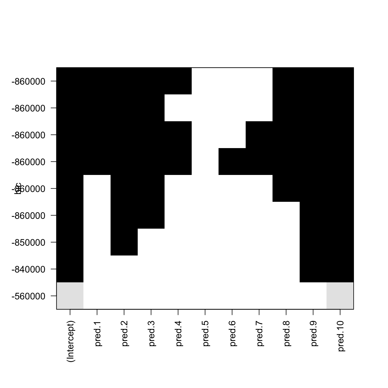
Figure 4.8: Best subsets for \(p=10\) predictors returned by leaps::regsubsets. The vertical axis indicates the sorting in terms of the BIC (the top positions contain the best models in terms of the BIC). White color indicates that the predictor is not included in the model and black that it is included. The \(p\) models obtained with the best subsets of \(1\leq r\leq p\) out of \(p\) predictors are displayed. Note that the vertical ordering does not necessarily coincide with \(r=1,\ldots,p\).
# Summarize (otherwise regsubsets's output is hard to decipher)
subs <- summary(reg)
subs
## Subset selection object
## 10 Variables  (and intercept)
##         Forced in Forced out
## pred.1      FALSE      FALSE
## pred.2      FALSE      FALSE
## pred.3      FALSE      FALSE
## pred.4      FALSE      FALSE
## pred.5      FALSE      FALSE
## pred.6      FALSE      FALSE
## pred.7      FALSE      FALSE
## pred.8      FALSE      FALSE
## pred.9      FALSE      FALSE
## pred.10     FALSE      FALSE
## 1 subsets of each size up to 9
## Selection Algorithm: exhaustive
##          pred.1 pred.2 pred.3 pred.4 pred.5 pred.6 pred.7 pred.8 pred.9 pred.10
## 1  ( 1 ) " "    " "    " "    " "    " "    " "    " "    " "    " "    "*"
## 2  ( 1 ) " "    " "    " "    " "    " "    " "    " "    " "    "*"    "*"
## 3  ( 1 ) " "    "*"    " "    " "    " "    " "    " "    " "    "*"    "*"
## 4  ( 1 ) " "    "*"    "*"    " "    " "    " "    " "    " "    "*"    "*"
## 5  ( 1 ) " "    "*"    "*"    " "    " "    " "    " "    "*"    "*"    "*"
## 6  ( 1 ) "*"    "*"    "*"    " "    " "    " "    " "    "*"    "*"    "*"
## 7  ( 1 ) "*"    "*"    "*"    "*"    " "    " "    " "    "*"    "*"    "*"
## 8  ( 1 ) "*"    "*"    "*"    "*"    " "    " "    "*"    "*"    "*"    "*"
## 9  ( 1 ) "*"    "*"    "*"    "*"    " "    "*"    "*"    "*"    "*"    "*"

# Lots of useful information
str(subs, 1)
## List of 8
##  $ which : logi [1:9, 1:11] TRUE TRUE TRUE TRUE TRUE TRUE ...
##   ..- attr(*, "dimnames")=List of 2
##  $ rsq   : num [1:9] 0.428 0.567 0.574 0.576 0.577 ...
##  $ rss   : num [1:9] 1352680 1023080 1006623 1003763 1001051 ...
##  $ adjr2 : num [1:9] 0.428 0.567 0.574 0.576 0.577 ...
##  $ cp    : num [1:9] 354480 24444 7968 5106 2392 ...
##  $ bic   : num [1:9] -558604 -837860 -854062 -856894 -859585 ...
##  $ outmat: chr [1:9, 1:10] " " " " " " " " ...
##   ..- attr(*, "dimnames")=List of 2
##  $ obj   :List of 27
##   ..- attr(*, "class")= chr "regsubsets"
##  - attr(*, "class")= chr "summary.regsubsets"

# Get the model with lowest BIC
subs$which
##   (Intercept) pred.1 pred.2 pred.3 pred.4 pred.5 pred.6 pred.7 pred.8 pred.9 pred.10
## 1        TRUE  FALSE  FALSE  FALSE  FALSE  FALSE  FALSE  FALSE  FALSE  FALSE    TRUE
## 2        TRUE  FALSE  FALSE  FALSE  FALSE  FALSE  FALSE  FALSE  FALSE   TRUE    TRUE
## 3        TRUE  FALSE   TRUE  FALSE  FALSE  FALSE  FALSE  FALSE  FALSE   TRUE    TRUE
## 4        TRUE  FALSE   TRUE   TRUE  FALSE  FALSE  FALSE  FALSE  FALSE   TRUE    TRUE
## 5        TRUE  FALSE   TRUE   TRUE  FALSE  FALSE  FALSE  FALSE   TRUE   TRUE    TRUE
## 6        TRUE   TRUE   TRUE   TRUE  FALSE  FALSE  FALSE  FALSE   TRUE   TRUE    TRUE
## 7        TRUE   TRUE   TRUE   TRUE   TRUE  FALSE  FALSE  FALSE   TRUE   TRUE    TRUE
## 8        TRUE   TRUE   TRUE   TRUE   TRUE  FALSE  FALSE   TRUE   TRUE   TRUE    TRUE
## 9        TRUE   TRUE   TRUE   TRUE   TRUE  FALSE   TRUE   TRUE   TRUE   TRUE    TRUE
subs$bic
## [1] -558603.7 -837859.9 -854062.3 -856893.8 -859585.3 -861936.5 -861939.3 -861932.3 -861918.6
subs$which[which.min(subs$bic), ]
## (Intercept)      pred.1      pred.2      pred.3      pred.4      pred.5      pred.6      pred.7      pred.8      pred.9
##        TRUE        TRUE        TRUE        TRUE        TRUE       FALSE       FALSE       FALSE        TRUE        TRUE
##     pred.10
##        TRUE

# Show the display in Figure 4.6
subs$which[order(subs$bic), ]
##   (Intercept) pred.1 pred.2 pred.3 pred.4 pred.5 pred.6 pred.7 pred.8 pred.9 pred.10
## 7        TRUE   TRUE   TRUE   TRUE   TRUE  FALSE  FALSE  FALSE   TRUE   TRUE    TRUE
## 6        TRUE   TRUE   TRUE   TRUE  FALSE  FALSE  FALSE  FALSE   TRUE   TRUE    TRUE
## 8        TRUE   TRUE   TRUE   TRUE   TRUE  FALSE  FALSE   TRUE   TRUE   TRUE    TRUE
## 9        TRUE   TRUE   TRUE   TRUE   TRUE  FALSE   TRUE   TRUE   TRUE   TRUE    TRUE
## 5        TRUE  FALSE   TRUE   TRUE  FALSE  FALSE  FALSE  FALSE   TRUE   TRUE    TRUE
## 4        TRUE  FALSE   TRUE   TRUE  FALSE  FALSE  FALSE  FALSE  FALSE   TRUE    TRUE
## 3        TRUE  FALSE   TRUE  FALSE  FALSE  FALSE  FALSE  FALSE  FALSE   TRUE    TRUE
## 2        TRUE  FALSE  FALSE  FALSE  FALSE  FALSE  FALSE  FALSE  FALSE   TRUE    TRUE
## 1        TRUE  FALSE  FALSE  FALSE  FALSE  FALSE  FALSE  FALSE  FALSE  FALSE    TRUE

# It also works with ordinary linear models and it is much faster and
# informative than step
reg <- leaps::regsubsets(resp ~ ., data = big_data1, nvmax = p,
                         method = "backward")
subs <- summary(reg)
subs$bic
##  [1] -558603.7 -837859.9 -854062.3 -856893.8 -859585.3 -861936.5 -861939.3 -861932.3 -861918.6 -861904.8
subs$which[which.min(subs$bic), ]
## (Intercept)      pred.1      pred.2      pred.3      pred.4      pred.5      pred.6      pred.7      pred.8      pred.9
##        TRUE        TRUE        TRUE        TRUE        TRUE       FALSE       FALSE       FALSE        TRUE        TRUE
##     pred.10
##        TRUE

# Compare it with step
step(lm(resp ~ ., data = big_data1), trace = 0,
     direction = "backward", k = log(n))
##
## Call:
## lm(formula = resp ~ pred.1 + pred.2 + pred.3 + pred.4 + pred.8 +
##     pred.9 + pred.10, data = big_data1)
##
## Coefficients:
## (Intercept)       pred.1       pred.2       pred.3       pred.4       pred.8       pred.9      pred.10
##    1.002141    -0.973201    -0.286626    -0.053487    -0.004074     0.052076     0.284038     0.986651
Finally, let’s see an example on how to fit a linear model to a large dataset that does not fit in the RAM of most regular laptops. Imagine that you want to regress a response \(Y\) into a set of \(p=10\) predictors and the sample size is \(n=10^8.\) Merely storing the response and the predictors will take approximately \(8.2\) GB in RAM:
# Size of the response
print(object.size(rnorm(1e6)) * 1e2, units = "GB")
## 0.7 Gb

# Size of the predictors
print(object.size(rnorm(1e6)) * 1e2 * 10, units = "GB")
## 7.5 Gb
In addition to this, if lm was called, it will return the residuals, effects, and fitted.values slots (all vectors of length \(n,\) hence \(0.7 \times 3=2.1\) GB more). It will also return the qr decomposition of the design matrix and the model matrix (both are \(n\times (p + 1)\) matrices, so another \(8.2\times 2=16.4\) GB more). The final lm object will thus be at the very least, of size \(18.5\) GB. Clearly, this is not a very memory-friendly procedure.
A possible approach is to split the dataset and perform updates of the model in chunks of reasonable size. The next code provides a template for such approach using biglm and update.
# Linear regression with n = 10^8 and p = 10
n <- 10^8
p <- 10
beta <- seq(-1, 1, length.out = p)^5

# Number of chunks for splitting the dataset
n_chunks <- 1e3
n_small <- n / n_chunks

# Simulates reading the first chunk of data
set.seed(12345)
x <- matrix(rnorm(n_small * p), nrow = n_small, ncol = p)
x[, p] <- 2 * x[, 1] + rnorm(n_small, sd = 0.1)
x[, p - 1] <- 2 - x[, 2] + rnorm(n_small, sd = 0.5)
y <- 1 + x %*% beta + rnorm(n_small)

# First fit
big_mod <- biglm::biglm(y ~ x, data = data.frame(y, x))

# Update fit
# pb <- txtProgressBar(style = 3)
for (i in 2:n_chunks) {

  # Simulates reading the i-th chunk of data
  set.seed(12345 + i)
  x <- matrix(rnorm(n_small * p), nrow = n_small, ncol = p)
  x[, p] <- 2 * x[, 1] + rnorm(n_small, sd = 0.1)
  x[, p - 1] <- 2 - x[, 2] + rnorm(n_small, sd = 0.5)
  y <- 1 + x %*% beta + rnorm(n_small)

  # Update the fit
  big_mod <- update(big_mod, moredata = data.frame(y, x))

  # Progress
  # setTxtProgressBar(pb = pb, value = i / nChunks)

}

# Final model
summary(big_mod)
## Large data regression model: biglm::biglm(y ~ x, data = data.frame(y, x))
## Sample size =  100000000
##                Coef    (95%     CI)    SE      p
## (Intercept)  1.0003  0.9995  1.0011 4e-04 0.0000
## x1          -1.0015 -1.0055 -0.9975 2e-03 0.0000
## x2          -0.2847 -0.2852 -0.2843 2e-04 0.0000
## x3          -0.0531 -0.0533 -0.0529 1e-04 0.0000
## x4          -0.0041 -0.0043 -0.0039 1e-04 0.0000
## x5           0.0002  0.0000  0.0004 1e-04 0.0760
## x6          -0.0001 -0.0003  0.0001 1e-04 0.2201
## x7           0.0041  0.0039  0.0043 1e-04 0.0000
## x8           0.0529  0.0527  0.0531 1e-04 0.0000
## x9           0.2844  0.2840  0.2848 2e-04 0.0000
## x10          1.0007  0.9987  1.0027 1e-03 0.0000
print(object.size(big_mod), units = "KB")
## 7.8 Kbsummary of a biglm object yields slightly different significances for the coefficients than those of lm. The reason is that biglm employs \(\mathcal{N}(0,1)\)-approximations for the distributions of the \(t\)-tests instead of the exact \(t_{n-1}\) distribution. Obviously, if \(n\) is large, the differences are inappreciable.
References
For example, the class of unbiased estimators is a very important class in the theory of estimation, then yielding the concepts of Uniformly Minimum Variance Unbiased Estimator (UMVUE).↩︎
Remember that, for a vector \(\mathbf{x}\in\mathbb{R}^m,\) \(r\geq 1,\) the \(\ell^r\) norm (usually referred to as \(\ell^p\) norm, but renamed here to avoid confusion with the number of predictors) is defined as \(\|\mathbf{x}\|_r:=\big(\sum_{j=1}^m|x_j|^r\big)^{1/r}.\) The \(\ell^\infty\) norm is defined as \(\|\mathbf{x}\|_\infty:=\max_{1\leq j\leq m}|x_j|\) and it is satisfied that \(\lim_{r\to\infty}\|\mathbf{x}\|_r=\|\mathbf{x}\|_\infty,\) for all \(\mathbf{x}\in\mathbb{R}^m\).↩︎
Such as, for example, \(\text{RSS}(\boldsymbol{\beta})+\lambda\|\boldsymbol\beta_{-1}\|_r^r,\) for \(r\geq 1.\)↩︎
The function \(\|\mathbf{x}\|_r^r\) is convex if \(r\geq1.\) If \(0<r<1,\) \(\|\mathbf{x}\|_r^r\) is not convex.↩︎
The main exception being the ridge regression, as seen in Section 4.1.1.↩︎
In addition, \(\alpha\) can also be regarded as a tuning parameter. We do not deal with its data-driven selection in these notes, as this will imply a more costly optimization of the cross-validation on the pair \((\lambda,\alpha).\)↩︎
Recall that (4.5) can be seen as the Lagrangian of (4.6). Because of the convexity of the optimization problem, the minimizers of (4.5) and (4.6) do actually coincide.↩︎
If the linear model is employed, for generalized linear models the metric in the cross-validation function is not the squared difference between observations and fitted values.↩︎
The “significance” here is only approximate: \(\text{CV}_k(\hat\lambda_{k\text{-CV}})\pm\hat{\mathrm{SE}}(\text{CV}_k(\hat\lambda_{k\text{-CV}}))\) is not a valid confidence interval for the population CV error (e.g., the standard error is itself an estimate). The philosophy of the rule, however, mirrors that of a hypothesis test for the equality of CV errors of the two selected models: \(\hat\lambda_{k\text{-1SE}}\) is the largest \(\lambda\) for which such a test would not be rejected at a level loosely associated with one standard error.↩︎
Indeed, Section 4.1.3 shows that \(\hat\lambda_{k\text{-1SE}}\) seems to be surprisingly good in terms of consistently identifying the underlying model.↩︎
That is, that \(\bar{Y}=0\) and \(\bar{X}_j=0,\) \(j=1,\ldots,p.\)↩︎
If the data was not centered, then (4.8) would translate into \(\hat{\boldsymbol{\beta}}_{\lambda,0}=(\mathbb{X}^\top\mathbb{X}+\mathrm{diag}(0,\lambda,\stackrel{p}{\ldots},\lambda))^{-1}\mathbb{X}^\top\mathbf{Y},\) where \(\mathbb{X}\) is the \(n\times(p+1)\) design matrix with the first column consisting of ones.↩︎
This was the original motivation for ridge regression, a way of estimating \(\boldsymbol\beta\) beyond \(p\leq n.\) This property also holds for any other elastic net estimator (e.g., lasso) as long as \(\lambda>0.\)↩︎
If the eigenvalues of \(\mathbb{X}^\top\mathbb{X}\) are \(\eta_1\geq \ldots\geq \eta_p>0,\) then the eigenvalues of \(\mathbb{X}^\top\mathbb{X}+\lambda\mathbf{I}_p\) are \(\eta_1+\lambda\geq \ldots\geq \eta_p+\lambda>0\) (because the addition involves a constant diagonal matrix). Therefore, the determinant of \((\mathbb{X}^\top\mathbb{X})^{-1}\) is \(\prod_{j=1}^p\eta_j^{-1}\) and the determinant of \((\mathbb{X}^\top\mathbb{X}+\lambda\mathbf{I}_p)^{-1}\mathbb{X}^\top\mathbb{X}(\mathbb{X}^\top\mathbb{X}+\lambda\mathbf{I}_p)^{-1}\) is \(\prod_{j=1}^p\eta_j(\eta_j+\lambda)^{-2},\) which is smaller than \(\prod_{j=1}^p\eta_j^{-1}\) since \(\lambda\geq0.\)↩︎
Observe that the expectation of \(\hat{\boldsymbol{\beta}}_{\lambda,0}\) depends on \(n\)! This was not the case for the least squares estimator \(\hat{\boldsymbol{\beta}}.\) This dependency can be removed if we reparametrize the penalty parameter \(\lambda\) as \(\tilde{\lambda}:=\lambda/n\), so that \(\lambda=n\tilde{\lambda}\). In the scale \(\tilde{\lambda}\), the expectation of \(\hat{\boldsymbol{\beta}}_{\tilde{\lambda},0}\) is fixed with respect to \(n.\) The scale \(\tilde{\lambda}\) is indeed the one used by
glmnet: \(\lambda_{\texttt{glmnet}}=\tilde{\lambda}.\)↩︎Recall that, if the predictors are centered, scaled, and uncorrelated, \(\frac{n+\lambda}{n}\hat{\boldsymbol{\beta}}_{\lambda,0}\sim\mathcal{N}_{p}\left(\boldsymbol{\beta},\frac{\sigma^2}{n}\mathbf{I}_p\right)\) and the \(t\)-tests and CIs for \(\beta_j\) follow easily from here. In general, from (4.9) it follows that \(\left(\mathbf{I}_p+\lambda(\mathbb{X}^\top\mathbb{X})^{-1}\right)\hat{\boldsymbol{\beta}}_{\lambda,0}\sim\mathcal{N}_{p}\left(\boldsymbol{\beta},\sigma^2 (\mathbb{X}^\top\mathbb{X})^{-1}\right)\) as long as \(\mathbb{X}^\top\mathbb{X}\) is invertible, from where \(t\)-tests and CIs for \(\beta_j\) can be derived.↩︎
We employ the cyclic property of the trace operator: \(\mathrm{tr}(\mathbf{A}\mathbf{B}\mathbf{C})=\mathrm{tr}(\mathbf{C}\mathbf{A}\mathbf{B})=\mathrm{tr}(\mathbf{B}\mathbf{C}\mathbf{A})\) for any matrices \(\mathbf{A},\) \(\mathbf{B},\) and \(\mathbf{C}\) for which the multiplications are possible.↩︎
One quirk is that
glmnet::glmnetconsiders \(\frac{1}{2n}\text{RSS}(\boldsymbol{\beta})+\lambda\left(\alpha\|\boldsymbol\beta_{-1}\|_1+\frac{1-\alpha}{2}\|\boldsymbol\beta_{-1}\|_2^2\right)\) instead of (4.4), since \(\frac{1}{2n}\text{RSS}(\boldsymbol{\beta})\) is more related with the log-likelihood. This rescaling of \(\text{RSS}(\boldsymbol{\beta})\) affects the scale of \(\lambda.\)↩︎Another quirk is that “
glmnet::glmnetstandardizesyto have unit variance (using \(1/n\) rather than \(1/(n-1)\) formula) before computing its lambda sequence (and then unstandardizes the resulting coefficients)”.↩︎Understanding this statement as that the probability of lasso-selecting the predictors with slopes different from zero converges to one when \(n\to\infty.\)↩︎
The details are quite technical and can be checked in Theorems 1–4 in Zhao and Yu (2006).↩︎
An example for \(p=5\) predictors follows. If \(\boldsymbol{\beta}_{-1}=(1,-1,0,0,0)^\top,\) then there are \(q=2\) non-zero slopes. Therefore, \(\frac{c}{2q-1}<\frac{1}{3}\) and the strong irrepresentable condition holds if all the correlations between the predictors are strictly smaller than \(\frac{1}{3}.\)↩︎
Based on limited empirical evidence!↩︎
Yet \(\hat\lambda_{n\text{-1SE}}\) is much faster to compute that doing an exhaustive search with BIC!↩︎
For example, based on the data-driven penalization parameters \(\hat\lambda_{k\text{-CV}}\) or \(\hat\lambda_{k\text{-1SE}}.\)↩︎
Note that with this approach we assign to the more computationally efficient lasso the “hard work” of coming up with a set of relevant predictors from the whole dataset, whereas the betterment of that model is done with the more demanding stepwise regression (if the number of predictors is smaller than \(n\)).↩︎
Note that this is a random quantity, but we ignore this fact for the sake of exposition.↩︎
Therefore, usually not invertible.↩︎
We do not require the previous notation \(\boldsymbol{\beta}_{-1}\)!↩︎
They do not depend on \(\mathbf{c}\)!↩︎
Do not confuse them with \(Y_1,\ldots,Y_n,\) the notation employed in the rest of the sections for denoting the sample of the response \(Y.\)↩︎
Centering the responses and predictors is useful for removing the intercept term, allowing for simpler matricial versions.↩︎
The notation \(\mathbb{X}\) now stands for the design matrix \(\mathbb{X}\) without the column of ones (because the predictor variables and response are centered).↩︎
Employing the centered version of the univariate multiple linear model, as we have done in this section for the multivariate version.↩︎
Indeed, specifying the full distribution of \(\hat{\mathbf{B}}\) would require introducing the matrix normal distribution, a generalization of the \(p\)-dimensional normal seen in Section 1.2.↩︎
Observe how the covariance of the errors \(\varepsilon_j\) and \(\varepsilon_k,\) denoted by \(\sigma_{jk},\) is the responsible of the correlation between \(\hat{\boldsymbol{\beta}}_j\) and \(\hat{\boldsymbol{\beta}}_k\) in (4.22). If \(\sigma_{jk}=0,\) then \(\hat{\boldsymbol{\beta}}_j\) and \(\hat{\boldsymbol{\beta}}_k\) would be uncorrelated, thus independent because of their joint normality. Therefore, inference on \(\boldsymbol{\beta}_j\) and \(\boldsymbol{\beta}_k\) could be carried out separately.↩︎
If \(q=1,\) then \(\sum_{j=1}^p\|\mathbf{B}_j\|_2=\sum_{j=1}^p\sqrt{\beta_{j1}^2}=\sum_{j=1}^p|\beta_{j1}|.\)↩︎
This property would not hold if the penalty \(\sum_{i=1}^p\sum_{j=1}^q|\beta_{ij}|\) was considered.↩︎
The QR decomposition of the matrix \(\mathbb{X}\) of size \(n\times m\) is \(\mathbb{X}=\mathbf{Q}\mathbf{R}\) such that \(\mathbf{Q}\) is an \(n\times n\) orthogonal matrix and \(\mathbf{R}\) is an \(n\times m\) upper triangular matrix. This factorization is commonly used in numerical analysis for solving linear systems.↩︎
Not really exhaustive: the method behind it, due to Furnival and Wilson (1974), employs an ingenious branch and bound algorithm to remove most of the non-interesting models.↩︎