2 Linear models I: multiple linear model

The multiple linear model is a simple but useful statistical model. In short, it allows us to analyze the (assumed) linear relation between a response \(Y\) and multiple predictors, \(X_1,\ldots,X_p\) in a proper way:

\[\begin{align*} Y=\beta_0+\beta_1X_1+\beta_2X_2+\cdots+\beta_pX_p+\varepsilon \end{align*}\]

The simplest case corresponds to \(p=1,\) known as the simple linear model:

\[\begin{align*} Y=\beta_0+\beta_1X+\varepsilon \end{align*}\]

This model would be useful, for example, to predict \(Y\) given \(X\) from a sample \((X_1,Y_1),\ldots,(X_n,Y_n)\) such that its scatterplot is the one in Figure 2.1.

Figure 2.1: Scatterplot of a sample \((X_1,Y_1),\ldots,(X_n,Y_n)\) showing a linear pattern.

2.1 Case study: The Bordeaux equation

Calculate the winter rain and the harvest rain (in millimeters). Add summer heat in the vineyard (in degrees centigrade). Subtract 12.145. And what do you have? A very, very passionate argument over wine.

— “Wine Equation Puts Some Noses Out of Joint”, The New York Times, 04/03/1990.

Figure 2.2: ABC interview to Orley Ashenfelter, broadcast in 1992. Video also available here.

This case study is motivated by the study of Princeton professor Orley Ashenfelter (Ashenfelter, Ashmore, and Lalonde 1995) on the quality of red Bordeaux vintages. The study became mainstream after disputes with the wine press, especially with Robert Parker Jr., one of the most influential wine critics in America. You can see a short review of the story at the Financial Times¹⁴ and at the video in Figure 2.2.

Red Bordeaux wines have been produced in Bordeaux, one of the most famous and prolific wine regions in the world, in a very similar way for hundreds of years. However, the quality of vintages is largely variable from one season to another due to a long list of random factors, such as weather conditions. Because Bordeaux wines taste better when they are older,¹⁵ there is an incentive to store the young wines until they are mature. Due to the important difference in taste, it is hard to determine the quality of the wine when it is so young just by tasting it, because it will change substantially when the aged wine is in the market. Therefore, being able to predict the quality of a vintage is valuable information for investing resources, for determining a fair price for vintages, and for understanding what factors are affecting the wine quality. The purpose of this case study is to answer:

• Q1. Can we predict the quality of a vintage effectively?
• Q2. What is the interpretation of such prediction?

The wine.csv file contains 27 red Bordeaux vintages. The data is the same data¹⁶ originally employed by Ashenfelter, Ashmore, and Lalonde (1995), except for the inclusion of the variable Year, the exclusion of NAs and the reference price used for the wine. Each row has the following variables:

• Year: year in which grapes were harvested to make wine.
• Price: logarithm of the average market price for Bordeaux vintages according to a series of auctions. The price is relative to the price of the 1961 vintage, regarded as the best one ever recorded.
• WinterRain: winter rainfall (in mm).
• AGST: Average Growing Season Temperature (in Celsius degrees).
• HarvestRain: harvest rainfall (in mm).
• Age: age of the wine, measured in 1983 as the number of years stored in a cask.
• FrancePop: population of France at Year (in thousands).

The quality of the wine is quantified as the Price, a clever way of quantifying a qualitative measure. A portion of the data is shown in Table 2.1.

Table 2.1: First 15 rows of the wine dataset.

Year	Price	WinterRain	AGST	HarvestRain	Age	FrancePop
1952	7.4950	600	17.1167	160	31	43183.57
1953	8.0393	690	16.7333	80	30	43495.03
1955	7.6858	502	17.1500	130	28	44217.86
1957	6.9845	420	16.1333	110	26	45152.25
1958	6.7772	582	16.4167	187	25	45653.81
1959	8.0757	485	17.4833	187	24	46128.64
1960	6.5188	763	16.4167	290	23	46584.00
1961	8.4937	830	17.3333	38	22	47128.00
1962	7.3880	697	16.3000	52	21	48088.67
1963	6.7127	608	15.7167	155	20	48798.99
1964	7.3094	402	17.2667	96	19	49356.94
1965	6.2518	602	15.3667	267	18	49801.82
1966	7.7443	819	16.5333	86	17	50254.97
1967	6.8398	714	16.2333	118	16	50650.41
1968	6.2435	610	16.2000	292	15	51034.41

We will see along the chapter how to answer Q1 and Q2 and how to obtain quantitative insights on the effects of the predictors on the price. Before doing so, we need to introduce the required statistical machinery.

2.2 Model formulation and least squares

In order to simplify the introduction of the foundations of the linear model, we first present the simple linear model and then extend it to the multiple linear model.

2.2.1 Simple linear model

The simple linear model is constructed by assuming that the linear relation

\[\begin{align} Y = \beta_0 + \beta_1 X + \varepsilon \tag{2.1} \end{align}\]

holds between \(X\) and \(Y.\) In (2.1), \(\beta_0\) and \(\beta_1\) are known as the intercept and slope, respectively. The random variable \(\varepsilon\) has mean zero and is independent from \(X.\) It describes the error around the mean, or the effect of other variables that we do not model. Another way of looking at (2.1) is

\[\begin{align} \mathbb{E}[Y \mid X=x]=\beta_0+\beta_1x, \tag{2.2} \end{align}\]

since \(\mathbb{E}[\varepsilon \mid X=x]=0.\)

The LHS of (2.2) is the conditional expectation of \(Y\) given \(X.\) It represents how the mean of the random variable \(Y\) is changing according to a particular value \(x\) of the random variable \(X.\) With the RHS, what we are saying is that the mean of \(Y\) is changing in a linear fashion with respect to the value of \(X.\) Hence the clear interpretation of the coefficients:

• \(\beta_0\): is the mean of \(Y\) when \(X=0.\)
• \(\beta_1\): is the increment in the mean of \(Y\) for an increment of one unit in \(X=x.\)

If we have a sample \((X_1,Y_1),\ldots,(X_n,Y_n)\) for our random variables \(X\) and \(Y,\) we can estimate the unknown coefficients \(\beta_0\) and \(\beta_1.\) A possible way of doing so is by looking for certain optimality, for example the minimization of the Residual Sum of Squares (RSS):

\[\begin{align*} \text{RSS}(\beta_0,\beta_1):=\sum_{i=1}^n(Y_i-\beta_0-\beta_1X_i)^2. \end{align*}\]

In other words, we look for the estimators \((\hat\beta_0,\hat\beta_1)\) such that

\[\begin{align*} (\hat\beta_0,\hat\beta_1)=\arg\min_{(\beta_0,\beta_1)\in\mathbb{R}^2} \text{RSS}(\beta_0,\beta_1). \end{align*}\]

The motivation for minimizing the RSS is geometrical, as shown by Figure 2.3. We aim to minimize the squares of the distances of points projected vertically onto the line determined by \((\hat\beta_0,\hat\beta_1).\)

Figure 2.3: The effect of the kind of distance in the error criterion. The choices of intercept and slope that minimize the sum of squared distances for one kind of distance are not the optimal choices for a different kind of distance. Application available here.

It can be seen that the minimizers of the RSS¹⁷ are

\[\begin{align} \hat\beta_0=\bar{Y}-\hat\beta_1\bar{X},\quad \hat\beta_1=\frac{s_{xy}}{s_x^2},\tag{2.3} \end{align}\]

where:

• \(\bar{X}=\frac{1}{n}\sum_{i=1}^nX_i\) is the sample mean.
• \(s_x^2=\frac{1}{n}\sum_{i=1}^n(X_i-\bar{X})^2\) is the sample variance.¹⁸
• \(s_{xy}=\frac{1}{n}\sum_{i=1}^n(X_i-\bar{X})(Y_i-\bar{Y})\) is the sample covariance. It measures the degree of linear association between \(X_1,\ldots,X_n\) and \(Y_1,\ldots,Y_n.\) Once scaled by \(s_xs_y,\) it gives the sample correlation coefficient \(r_{xy}=\frac{s_{xy}}{s_xs_y}.\)

There are some important points hidden behind the choice of RSS as the error criterion for obtaining \((\hat\beta_0,\hat\beta_1)\):

• Why the vertical distances and not horizontal or perpendicular? Because we want to minimize the error in the prediction of \(Y\)! Note that the treatment of the variables is not symmetrical.
• Why the squares in the distances and not the absolute value? Due to mathematical convenience. Squares are nice to differentiate and are closely related to maximum likelihood estimation under the normal distribution (see Appendix B).

Let’s see how to obtain automatically the minimizers of the error in Figure 2.3 by the lm (linear model) function. The data of the figure has been generated with the following code:

# Generates 50 points from a N(0, 1): predictor and error
set.seed(34567)
x <- rnorm(n = 50)
eps <- rnorm(n = 50)

# Responses
yLin <- -0.5 + 1.5 * x + eps
yQua <- -0.5 + 1.5 * x^2 + eps
yExp <- -0.5 + 1.5 * 2^x + eps

# Data
leastSquares <- data.frame(x = x, yLin = yLin, yQua = yQua, yExp = yExp)

For a simple linear model, lm has the syntax lm(formula = response ~ predictor, data = data), where response and predictor are the names of two variables in the data frame data. Note that the LHS of ~ represents the response and the RHS the predictors.

# Call lm
lm(yLin ~ x, data = leastSquares)
## 
## Call:
## lm(formula = yLin ~ x, data = leastSquares)
## 
## Coefficients:
## (Intercept)            x  
##     -0.6154       1.3951
lm(yQua ~ x, data = leastSquares)
## 
## Call:
## lm(formula = yQua ~ x, data = leastSquares)
## 
## Coefficients:
## (Intercept)            x  
##      0.9710      -0.8035
lm(yExp ~ x, data = leastSquares)
## 
## Call:
## lm(formula = yExp ~ x, data = leastSquares)
## 
## Coefficients:
## (Intercept)            x  
##       1.270        1.007

# The lm object
mod <- lm(yLin ~ x, data = leastSquares)
mod
## 
## Call:
## lm(formula = yLin ~ x, data = leastSquares)
## 
## Coefficients:
## (Intercept)            x  
##     -0.6154       1.3951

# We can produce a plot with the linear fit easily
plot(x, yLin)
abline(coef = mod$coefficients, col = 2)

Figure 2.4: Linear fit for the data employed in Figure 2.3 minimizing the RSS.

# Access coefficients with $coefficients
mod$coefficients
## (Intercept)           x 
##  -0.6153744   1.3950973

# Compute the minimized RSS
sum((yLin - mod$coefficients[1] - mod$coefficients[2] * x)^2)
## [1] 41.02914
sum(mod$residuals^2)
## [1] 41.02914

# mod is a list of objects whose names are
names(mod)
##  [1] "coefficients"  "residuals"     "effects"       "rank"          "fitted.values" "assign"        "qr"           
##  [8] "df.residual"   "xlevels"       "call"          "terms"         "model"

Exercise 2.1 Check that you cannot improve the error in Figure 2.3 when using the coefficients given by lm, if vertical distances are selected. Check also that these coefficients are only optimal for vertical distances.

An interesting exercise is to check that lm is actually implementing the estimates given in (2.3):

# Covariance
Sxy <- cov(x, yLin)

# Variance
Sx2 <- var(x)

# Coefficients
beta1 <- Sxy / Sx2
beta0 <- mean(yLin) - beta1 * mean(x)
c(beta0, beta1)
## [1] -0.6153744  1.3950973

# Output from lm
mod <- lm(yLin ~ x, data = leastSquares)
mod$coefficients
## (Intercept)           x 
##  -0.6153744   1.3950973

The population regression coefficients, \((\beta_0,\beta_1),\) are not the same as the estimated regression coefficients, \((\hat\beta_0,\hat\beta_1)\):

• \((\beta_0,\beta_1)\) are the theoretical and always unknown quantities (except under controlled scenarios).
• \((\hat\beta_0,\hat\beta_1)\) are the estimates computed from the data. They are random variables, since they are computed from the random sample \((X_1,Y_1),\ldots,(X_n,Y_n).\)

In an abuse of notation, the term regression line is often used to denote both the theoretical (\(y=\beta_0+\beta_1x\)) and the estimated (\(y=\hat\beta_0+\hat\beta_1x\)) regression lines.

2.2.2 Case study application

Let’s get back to the wine dataset and compute some simple linear regressions. Prior to that, let’s begin by summarizing the information in Table 2.1 to get an idea of the structure of the data. For that, we first correctly import the dataset into R:

# Read data
wine <- read.table(file = "wine.csv", header = TRUE, sep = ",")

Now we can conduct a quick exploratory analysis to have insights into the data:

# Numerical -- marginal distributions
summary(wine)
##       Year          Price         WinterRain         AGST        HarvestRain         Age          FrancePop    
##  Min.   :1952   Min.   :6.205   Min.   :376.0   Min.   :14.98   Min.   : 38.0   Min.   : 3.00   Min.   :43184  
##  1st Qu.:1960   1st Qu.:6.508   1st Qu.:543.5   1st Qu.:16.15   1st Qu.: 88.0   1st Qu.: 9.50   1st Qu.:46856  
##  Median :1967   Median :6.984   Median :600.0   Median :16.42   Median :123.0   Median :16.00   Median :50650  
##  Mean   :1967   Mean   :7.042   Mean   :608.4   Mean   :16.48   Mean   :144.8   Mean   :16.19   Mean   :50085  
##  3rd Qu.:1974   3rd Qu.:7.441   3rd Qu.:705.5   3rd Qu.:17.01   3rd Qu.:185.5   3rd Qu.:22.50   3rd Qu.:53511  
##  Max.   :1980   Max.   :8.494   Max.   :830.0   Max.   :17.65   Max.   :292.0   Max.   :31.00   Max.   :55110

# Graphical -- pairwise relations with linear and "smooth" regressions
car::scatterplotMatrix(wine, col = 1, regLine = list(col = 2),
                       smooth = list(col.smooth = 4, col.spread = 4))

Figure 2.5: Scatterplot matrix for the wine dataset. The diagonal plots show density estimators of the pdf of each variable (see Section 6.1.2). The \((i,j)\)-th scatterplot shows the data of \(X_i\) vs. \(X_j,\) where the red line is the regression line of \(X_i\) (response) on \(X_j\) (predictor) and the blue curve represents a smoother that estimates nonparametrically the regression function of \(X_i\) on \(X_j\) (see Section 6.2). The dashed blue curves are the confidence intervals associated to the nonparametric smoother.

As we can see, Year and FrancePop are very dependent, and Year and Age are perfectly dependent. This is so because Age = 1983 - Year. Therefore, we opt to remove the predictor Year and use it to set the case names, which can be helpful later for identifying outliers:

# Set row names to Year -- useful for outlier identification
row.names(wine) <- wine$Year
wine$Year <- NULL

Remember that the objective is to predict Price. Based on the above matrix scatterplot, the best we can predict Price by a simple linear regression seems to be with AGST or HarvestRain. Let’s see which one yields the larger \(R^2,\) which, as we will see in Section 2.7.1, is indicative of the performance of the linear model.

# Price ~ AGST
modAGST <- lm(Price ~ AGST, data = wine)

# Summary of the model
summary(modAGST)
## 
## Call:
## lm(formula = Price ~ AGST, data = wine)
## 
## Residuals:
##      Min       1Q   Median       3Q      Max 
## -0.78370 -0.23827 -0.03421  0.29973  0.90198 
## 
## Coefficients:
##             Estimate Std. Error t value Pr(>|t|)    
## (Intercept)  -3.5469     2.3641  -1.500 0.146052    
## AGST          0.6426     0.1434   4.483 0.000143 ***
## ---
## Signif. codes:  0 '***' 0.001 '**' 0.01 '*' 0.05 '.' 0.1 ' ' 1
## 
## Residual standard error: 0.4819 on 25 degrees of freedom
## Multiple R-squared:  0.4456, Adjusted R-squared:  0.4234 
## F-statistic: 20.09 on 1 and 25 DF,  p-value: 0.0001425

# The summary is also an object
sumModAGST <- summary(modAGST)
names(sumModAGST)
##  [1] "call"          "terms"         "residuals"     "coefficients"  "aliased"       "sigma"         "df"           
##  [8] "r.squared"     "adj.r.squared" "fstatistic"    "cov.unscaled"

# R^2
sumModAGST$r.squared
## [1] 0.4455894

Exercise 2.2 Complete the analysis by computing the linear models Price ~ FrancePop, Price ~ Age, Price ~ WinterRain, and Price ~ HarvestRain. Name them as modFrancePop, modAge, modWinterRain, and modHarvestRain. Obtain their \(R^2\)’s and display them in a table like:

Predictor	\(R^2\)
AGST	\(0.4456\)
HarvestRain	\(0.2572\)
FrancePop	\(0.2314\)
Age	\(0.2120\)
WinterRain	\(0.0181\)

It seems that none of these simple linear models on their own are properly explaining Price. Intuitively, it would make sense to combine them together to achieve a better explanation of Price. Let’s see how to do that with a more advanced model.

2.2.3 Multiple linear model

The multiple linear model extends the simple linear model by describing the relation between several random variables \(X_1,\ldots,X_p\;\)¹⁹ and \(Y.\) Therefore, as before, the multiple linear model is constructed by assuming that the linear relation

\[\begin{align} Y = \beta_0 + \beta_1 X_1 + \cdots + \beta_p X_p + \varepsilon \tag{2.4} \end{align}\]

holds between the predictors \(X_1,\ldots,X_p\) and the response \(Y.\) In (2.4), \(\beta_0\) is the intercept and \(\beta_1,\ldots,\beta_p\) are the slopes, respectively. The random variable \(\varepsilon\) has mean zero and is independent from \(X_1,\ldots,X_p.\) Another way of looking at (2.4) is

\[\begin{align} \mathbb{E}[Y \mid X_1=x_1,\ldots,X_p=x_p]=\beta_0+\beta_1x_1+\cdots+\beta_px_p, \tag{2.5} \end{align}\]

since \(\mathbb{E}[\varepsilon \mid X_1=x_1,\ldots,X_p=x_p]=0.\)

The LHS of (2.5) is the conditional expectation of \(Y\) given \(X_1,\ldots,\) \(X_p.\) It represents how the mean of the random variable \(Y\) is changing, now according to particular values of several predictors. With the RHS, what we are saying is that the mean of \(Y\) is changing in a linear fashion with respect to the values of \(X_1,\ldots,X_p.\) Hence the neat interpretation of the coefficients:

• \(\beta_0\): is the mean of \(Y\) when \(X_1=\cdots=X_p=0.\)
• \(\beta_j,\) \(1\leq j\leq p\): is the increment in the mean of \(Y\) for an increment of one unit in \(X_j=x_j,\) provided that the rest of predictors \(X_1,\ldots,X_{j-1},X_{j+1},\ldots,X_p\) remain constant.

Figure 2.6 illustrates the geometrical interpretation of a multiple linear model: a hyperplane in \(\mathbb{R}^{p+1}.\) If \(p=1,\) the hyperplane is actually a line, the regression line for simple linear regression. If \(p=2,\) then the regression plane can be visualized in a \(3\)-dimensional plot.

The estimation of \(\beta_0,\beta_1,\ldots,\beta_p\) is done as in simple linear regression by minimizing the RSS, which now accounts for the sum of squared distances of the data to the vertical projections on the hyperplane. Before doing so, we need to introduce some helpful matrix notation:

• A sample of \((X_1,\ldots,X_p,Y)\) is denoted as \(\{(X_{i1},\ldots,X_{ip},Y_i)\}_{i=1}^n,\) where \(X_{ij}\) is the \(i\)-th observation of the \(j\)-th predictor \(X_j.\) We denote with \(\mathbf{X}_i:=(X_{i1},\ldots,X_{ip})\) to the \(i\)-th observation of \((X_1,\ldots,X_p),\) so the sample simplifies to \(\{(\mathbf{X}_{i},Y_i)\}_{i=1}^n.\)

• The design matrix contains all the information of the predictors plus a column of ones

\[\begin{align*} \mathbf{X}:=\begin{pmatrix} 1 & X_{11} & \cdots & X_{1p}\\ \vdots & \vdots & \ddots & \vdots\\ 1 & X_{n1} & \cdots & X_{np} \end{pmatrix}_{n\times(p+1)}. \end{align*}\]

• The vector of responses \(\mathbf{Y},\) the vector of coefficients \(\boldsymbol{\beta},\) and the vector of errors \(\boldsymbol{\varepsilon}\) are, respectively,

\[\begin{align*} \mathbf{Y}:=\begin{pmatrix} Y_1 \\ \vdots \\ Y_n \end{pmatrix}_{n\times 1},\quad\boldsymbol{\beta}:=\begin{pmatrix} \beta_0 \\ \beta_1 \\ \vdots \\ \beta_p \end{pmatrix}_{(p+1)\times 1}\text{, and } \boldsymbol{\varepsilon}:=\begin{pmatrix} \varepsilon_1 \\ \vdots \\ \varepsilon_n \end{pmatrix}_{n\times 1}. \end{align*}\]

Thanks to the matrix notation, we can turn the sample version²⁰ of the multiple linear model, namely

\[\begin{align*} Y_i=\beta_0 + \beta_1 X_{i1} + \cdots +\beta_p X_{ip} + \varepsilon_i,\quad i=1,\ldots,n, \end{align*}\]

into something as compact as

\[\begin{align*} \mathbf{Y}=\mathbf{X}\boldsymbol{\beta}+\boldsymbol{\varepsilon}. \end{align*}\]

Figure 2.6: The least squares regression plane \(y=\hat\beta_0+\hat\beta_1x_1+\hat\beta_2x_2\) and its dependence on the kind of squared distance considered. Application available here.

Recall that if \(p=1\) we recover the simple linear model. In this case:

\[\begin{align*} \mathbf{X}=\begin{pmatrix} 1 & X_{11}\\ \vdots & \vdots\\ 1 & X_{n1} \end{pmatrix}_{n\times2}\text{ and } \boldsymbol{\beta}=\begin{pmatrix} \beta_0 \\ \beta_1 \end{pmatrix}_{2\times 1}. \end{align*}\]

With this notation, the RSS for the multiple linear regression is

\[\begin{align} \text{RSS}(\boldsymbol{\beta}):=&\,\sum_{i=1}^n(Y_i-\beta_0-\beta_1X_{i1}-\cdots-\beta_pX_{ip})^2\nonumber\\ =&\,(\mathbf{Y}-\mathbf{X}\boldsymbol{\beta})^\top(\mathbf{Y}-\mathbf{X}\boldsymbol{\beta}).\tag{2.6} \end{align}\]

The RSS aggregates the squared vertical distances from the data to a regression plane given by \(\boldsymbol{\beta}.\) The least squares estimators are the minimizers of the RSS²¹:

\[\begin{align*} \hat{\boldsymbol{\beta}}:=\arg\min_{\boldsymbol{\beta}\in\mathbb{R}^{p+1}} \text{RSS}(\boldsymbol{\beta}). \end{align*}\]

Luckily, thanks to the matrix form of (2.6), it is possible²² to compute a closed-form expression for the least squares estimates:

\[\begin{align} \hat{\boldsymbol{\beta}}=(\mathbf{X}^\top\mathbf{X})^{-1}\mathbf{X}^\top\mathbf{Y}.\tag{2.7} \end{align}\]

There are some similarities between (2.7) and \(\hat\beta_1=(s_x^2)^{-1}\) \(s_{xy}\) from the simple linear model: both are related to the covariance between \(\mathbf{X}\) and \(Y\) weighted by the variance of \(\mathbf{X}.\)

Let’s check that indeed the coefficients given by lm are the ones given by (2.7). For that purpose we consider the leastSquares3D data frame in the least-squares-3D.RData dataset. Among other variables, the data frame contains the response yLin and the predictors x1 and x2.

load(file = "least-squares-3D.RData")

Let’s compute the coefficients of the regression of yLin on the predictors x1 and x2, which is denoted by yLin ~ x1 + x2. Note the use of + for including all the predictors. This does not mean that they are all added and then the regression is done on the sum.²³ Instead, this syntax is designed to resemble the mathematical form of the multiple linear model.

# Output from lm
mod <- lm(yLin ~ x1 + x2, data = leastSquares3D)
mod$coefficients
## (Intercept)          x1          x2 
##  -0.5702694   0.4832624   0.3214894

# Matrix X
X <- cbind(1, leastSquares3D$x1, leastSquares3D$x2)

# Vector Y
Y <- leastSquares3D$yLin

# Coefficients
beta <- solve(t(X) %*% X) %*% t(X) %*% Y
# %*% multiplies matrices
# solve() computes the inverse of a matrix
# t() transposes a matrix
beta
##            [,1]
## [1,] -0.5702694
## [2,]  0.4832624
## [3,]  0.3214894

Exercise 2.3 Compute \(\hat{\boldsymbol{\beta}}\) for the regressions yLin ~ x1 + x2, yQua ~ x1 + x2, and yExp ~ x2 + x3 using:

1. Equation (2.7) and
2. the function lm.

Check that both are the same.

Once we have the least squares estimates \(\hat{\boldsymbol{\beta}},\) we can define the next concepts:

• The fitted values \(\hat Y_1,\ldots,\hat Y_n,\) where

  \[\begin{align*} \hat Y_i:=\hat\beta_0+\hat\beta_1X_{i1}+\cdots+\hat\beta_pX_{ip},\quad i=1,\ldots,n. \end{align*}\]

  They are the vertical projections of \(Y_1,\ldots,Y_n\) onto the fitted plane (see Figure 2.6). In matrix form, substituting (2.6)

  \[\begin{align*} \hat{\mathbf{Y}}=\mathbf{X}\hat{\boldsymbol{\beta}}=\mathbf{X}(\mathbf{X}^\top\mathbf{X})^{-1}\mathbf{X}^\top\mathbf{Y}=\mathbf{H}\mathbf{Y}, \end{align*}\]

  where \(\mathbf{H}:=\mathbf{X}(\mathbf{X}^\top\mathbf{X})^{-1}\mathbf{X}^\top\) is called the hat matrix because it “puts the hat on \(\mathbf{Y}\)”. What it does is to project \(\mathbf{Y}\) into the regression plane (see Figure 2.6).

• The residuals (or estimated errors) \(\hat \varepsilon_1,\ldots,\hat \varepsilon_n,\) where

  \[\begin{align*} \hat\varepsilon_i:=Y_i-\hat Y_i,\quad i=1,\ldots,n. \end{align*}\]

  They are the vertical distances between actual data and fitted data.

These two objects are present in the output of lm:

# Fitted values
mod$fitted.values

# Residuals
mod$residuals

We conclude with an important insight on the relation of multiple and simple linear regressions that is illustrated in Figure 2.7. The data used in that figure is:

set.seed(212542)
n <- 100
x1 <- rnorm(n, sd = 2)
x2 <- rnorm(n, mean = x1, sd = 3)
y <- 1 + 2 * x1 - x2 + rnorm(n, sd = 1)
data <- data.frame(x1 = x1, x2 = x2, y = y)

Consider the multiple linear model \(Y=\beta_0+\beta_1X_1+\beta_2X_2\) \(+\varepsilon_1\) and its associated simple linear models \(Y=\alpha_0+\alpha_1X_1+\varepsilon_2\) and \(Y=\gamma_0+\gamma_1X_2+\varepsilon_3,\) where \(\varepsilon_1,\varepsilon_2,\varepsilon_3\) are random errors. Assume that we have a sample \(\{(X_{i1},X_{i2},Y_i)\}_{i=1}^n.\) Then, in general, \(\hat\alpha_0\neq\hat\beta_0\neq\hat\gamma_0,\) \(\hat\alpha_1\neq\hat\beta_1,\) and \(\hat\gamma_1\neq\hat\beta_2.\) Even if \(\alpha_0=\beta_0=\gamma_0,\) \(\alpha_1=\beta_1,\) and \(\gamma_1=\beta_2.\) That is, in general, the inclusion of a new predictor changes the coefficient estimates of the rest of predictors.

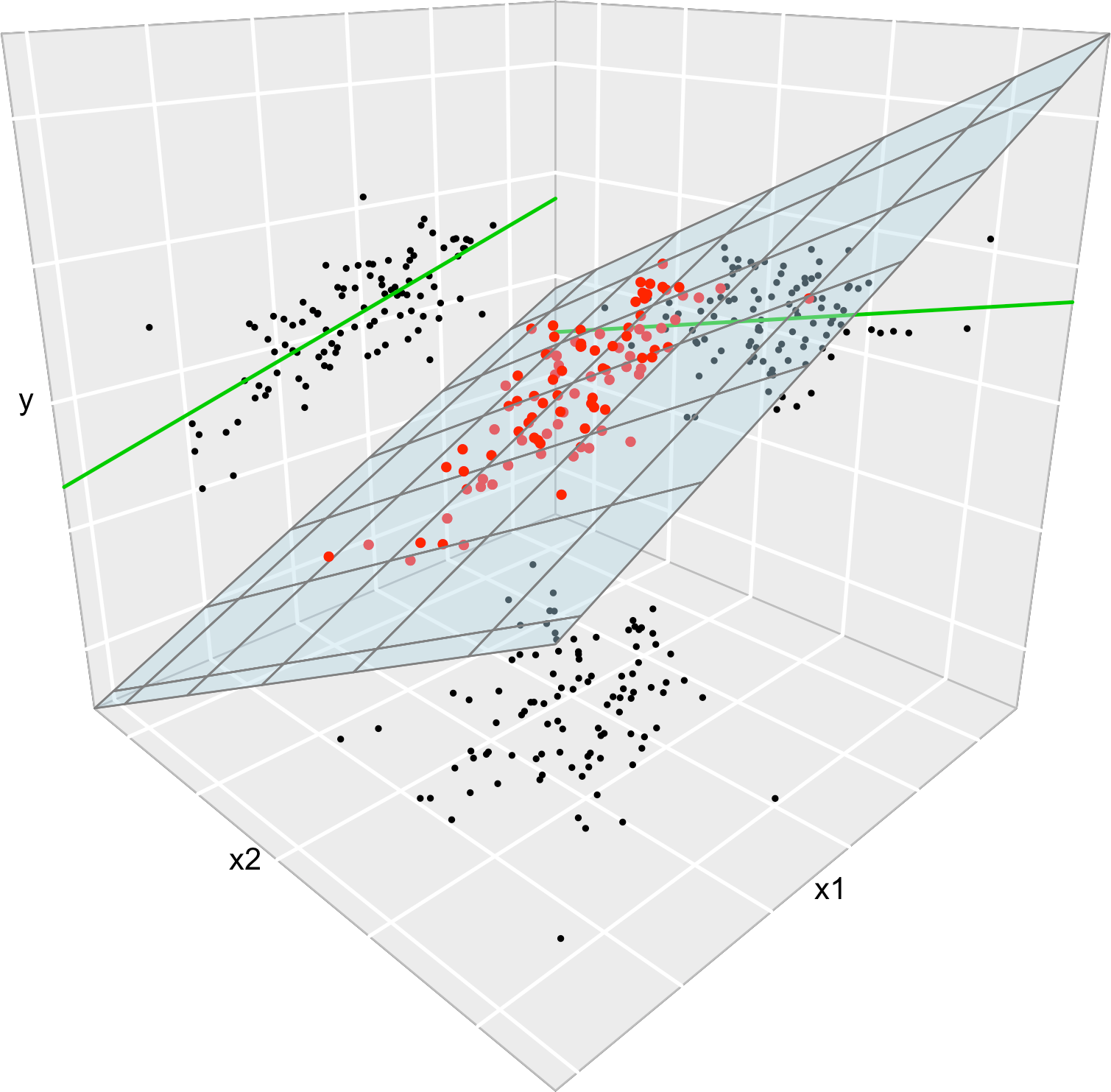
Figure 2.7: The regression plane (blue) of \(Y\) on \(X_1\) and \(X_2\) and its relation with the simple linear regressions (green lines) of \(Y\) on \(X_1\) and of \(Y\) on \(X_2.\) The red points represent the sample for \((X_1,X_2,Y)\) and the black points the sample projections for \((X_1,X_2)\) (bottom), \((X_1,Y)\) (left), and \((X_2,Y)\) (right). As it can be seen, the regression plane does not extend the simple linear regressions.

Exercise 2.4 With the above data, check how the fitted coefficients change for y ~ x1, y ~ x2, and y ~ x1 + x2.

2.2.4 Case study application

A natural step now is to extend these simple regressions to increase both the \(R^2\) and the prediction accuracy for Price by means of the multiple linear regression:

# Regression on all the predictors
modWine1 <- lm(Price ~ Age + AGST + FrancePop + HarvestRain + WinterRain,
               data = wine)

# A shortcut
modWine1 <- lm(Price ~ ., data = wine)
modWine1
## 
## Call:
## lm(formula = Price ~ ., data = wine)
## 
## Coefficients:
## (Intercept)   WinterRain         AGST  HarvestRain          Age    FrancePop  
##  -2.343e+00    1.153e-03    6.144e-01   -3.837e-03    1.377e-02   -2.213e-05

# Summary
summary(modWine1)
## 
## Call:
## lm(formula = Price ~ ., data = wine)
## 
## Residuals:
##      Min       1Q   Median       3Q      Max 
## -0.46541 -0.24133  0.00413  0.18974  0.52495 
## 
## Coefficients:
##               Estimate Std. Error t value Pr(>|t|)    
## (Intercept) -2.343e+00  7.697e+00  -0.304  0.76384    
## WinterRain   1.153e-03  4.991e-04   2.311  0.03109 *  
## AGST         6.144e-01  9.799e-02   6.270 3.22e-06 ***
## HarvestRain -3.837e-03  8.366e-04  -4.587  0.00016 ***
## Age          1.377e-02  5.821e-02   0.237  0.81531    
## FrancePop   -2.213e-05  1.268e-04  -0.175  0.86313    
## ---
## Signif. codes:  0 '***' 0.001 '**' 0.01 '*' 0.05 '.' 0.1 ' ' 1
## 
## Residual standard error: 0.293 on 21 degrees of freedom
## Multiple R-squared:  0.8278, Adjusted R-squared:  0.7868 
## F-statistic: 20.19 on 5 and 21 DF,  p-value: 2.232e-07

The fitted regression is Price \(= -2.343 + 0.013\,\times\) Age \(+ 0.614\,\times\) AGST \(- 0.000\,\times\) FrancePop \(- 0.003\,\times\) HarvestRain \(+ 0.001\,\times\) WinterRain. Recall that the 'Multiple R-squared' has almost doubled with respect to the best simple linear regression! This tells us that combining several predictors may lead to important performance gains in the prediction of the response. However, note that the \(R^2\) of the multiple linear model is not the sum of the \(R^2\)’s of the simple linear models. The performance gain of combining predictors is hard to anticipate from the single-predictor models and depends on the dependence among the predictors.

2.3 Assumptions of the model

A natural²⁴ question to ask is: “Why do we need assumptions?” The answer is that we need probabilistic assumptions to ground statistical inference about the model parameters. Or, in other words, to quantify the variability of the estimator \(\hat{\boldsymbol{\beta}}\) and to infer properties about the unknown population coefficients \(\boldsymbol{\beta}\) from the sample \(\{(\mathbf{X}_i, Y_i)\}_{i=1}^n.\)

The assumptions of the multiple linear model are:

1. Linearity: \(\mathbb{E}[Y \mid X_1=x_1,\ldots,X_p=x_p]=\beta_0+\beta_1x_1+\cdots+\beta_px_p.\)
2. Homoscedasticity: \(\mathbb{V}\text{ar}[\varepsilon \mid X_1=x_1,\ldots,X_p=x_p]=\sigma^2.\)
3. Normality: \(\varepsilon\sim\mathcal{N}(0,\sigma^2).\)
4. Independence of the errors: \(\varepsilon_1,\ldots,\varepsilon_n\) are independent (or uncorrelated, \(\mathbb{E}[\varepsilon_i\varepsilon_j]=0,\) \(i\neq j,\) since they are assumed to be normal).

A good one-line summary of the linear model is the following (independence is implicit)

\[\begin{align} Y \mid (X_1=x_1,\ldots,X_p=x_p)\sim \mathcal{N}(\beta_0+\beta_1x_1+\cdots+\beta_px_p,\sigma^2).\tag{2.8} \end{align}\]

Recall that, except for assumption iv, the rest are expressed in terms of the random variables, not in terms of the sample. Thus they are population versions, rather than sample versions. It is however trivial to express (2.8) in terms of assumptions about the sample \(\{(\mathbf{X}_i,Y_i)\}_{i=1}^n\):

\[\begin{align} Y_i \mid (X_{i1}=x_{i1},\ldots,X_{ip}=x_{ip})\sim \mathcal{N}(\beta_0+\beta_1x_{i1}+\cdots+\beta_px_{ip},\sigma^2),\tag{2.9} \end{align}\]

with \(Y_1,\ldots,Y_n\) being independent conditionally on the sample of predictors. Equivalently stated in a compact matrix way, the assumptions of the model on the sample are:

\[\begin{align} \mathbf{Y} \mid \mathbf{X}\sim\mathcal{N}_n(\mathbf{X}\boldsymbol{\beta},\sigma^2\mathbf{I}).\tag{2.10} \end{align}\]

Figures 2.10 and 2.11 represent situations where the assumptions of the model for \(p=1\) are respected and violated, respectively.

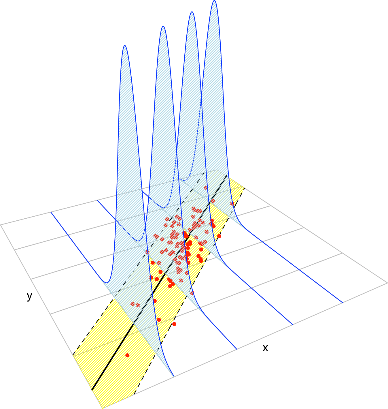
Figure 2.8: The key concepts of the simple linear model. The red points represent a sample with population regression line \(y=\beta_0+\beta_1x\) given by the black line. The yellow band denotes where \(95\%\) of the data is, according to the model. The blue densities represent the conditional density of \(Y\) given \(X=x,\) whose means lie in the regression line.

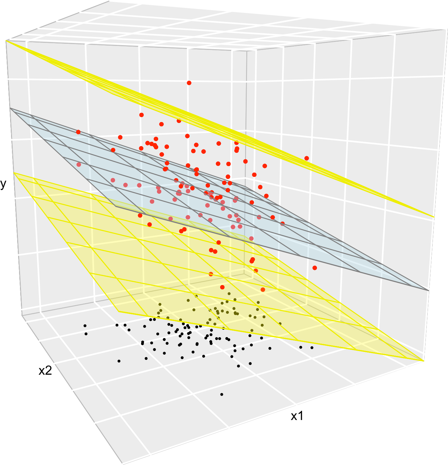
Figure 2.9: The key concepts of the multiple linear model when \(p=2.\) The red points represent a sample with population regression plane \(y=\beta_0+\beta_1x_1+\beta_2x_2\) given by the blue plane. The black points represent the associated observations of the predictors. The space between the yellow planes denotes where \(95\%\) of the data is, according to the model.

Figure 2.12 represents situations where the assumptions of the model are respected and violated, for the situation with two predictors. Clearly, the inspection of the scatterplots for identifying strange patterns is more complicated than in simple linear regression – and here we are dealing only with two predictors.

Figure 2.10: Perfectly valid simple linear models (all the assumptions are verified).

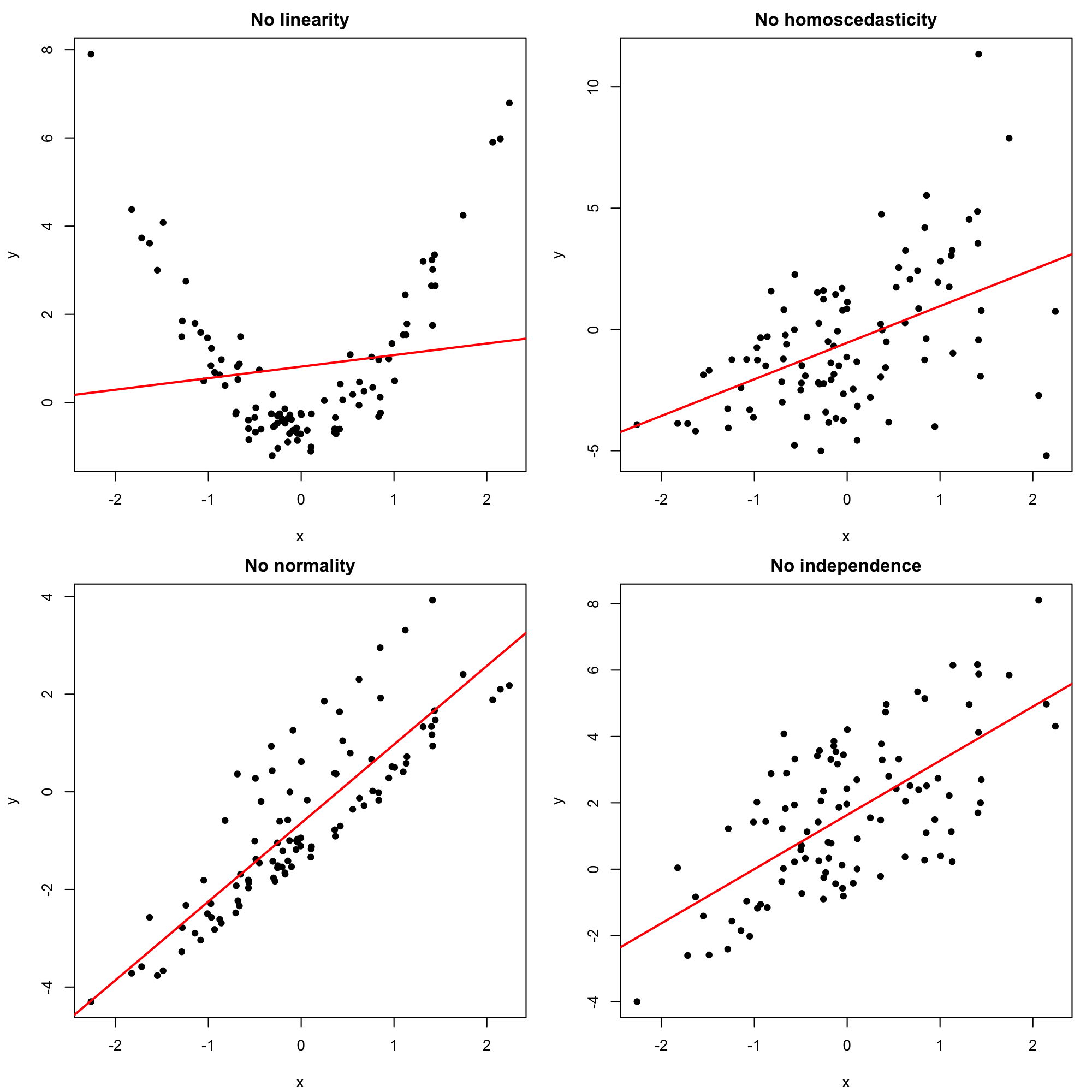
Figure 2.11: Problematic simple linear models (a single assumption does not hold).

Figure 2.12: Valid (all the assumptions are verified) and problematic (a single assumption does not hold) multiple linear models, when there are two predictors. Application available here.

Exercise 2.5 The dataset assumptions.RData contains the variables x1, …, x9 and y1, …, y9. For each regression y1 ~ x1, …, y9 ~ x9:

1. Check whether the assumptions of the linear model are being satisfied (make a scatterplot with a regression line).
2. State which assumption(s) are violated and justify your answer.

2.4 Inference for model parameters

The assumptions introduced in the previous section allow us to specify what is the distribution of the random vector \(\hat{\boldsymbol{\beta}}.\) The distribution is derived conditionally on the predictors’ sample \(\mathbf{X}_1,\ldots,\mathbf{X}_n.\) In other words, we assume that the randomness of \(\mathbf{Y}=\mathbf{X}\boldsymbol{\beta}+\boldsymbol{\varepsilon}\) comes only from the error terms and not from the predictors.²⁵ To denote this, we employ lowercase for the predictors’ sample \(\mathbf{x}_1,\ldots,\mathbf{x}_n.\)

2.4.1 Distributions of the fitted coefficients

The distribution of \(\hat{\boldsymbol{\beta}}\) is:

\[\begin{align} \hat{\boldsymbol{\beta}}\sim\mathcal{N}_{p+1}\left(\boldsymbol{\beta},\sigma^2(\mathbf{X}^\top\mathbf{X})^{-1}\right). \tag{2.11} \end{align}\]

This result can be obtained from the form of \(\hat{\boldsymbol{\beta}}\) given in (2.7), the sample version of the model assumptions given in (2.10), and the linear transformation property of a normal given in (1.4). Equation (2.11) implies that the marginal distribution of \(\hat\beta_j\) is

\[\begin{align} \hat{\beta}_j\sim\mathcal{N}\left(\beta_j,\mathrm{SE}(\hat\beta_j)^2\right),\tag{2.12} \end{align}\]

where \(\mathrm{SE}(\hat\beta_j)\) is the standard error, \(\mathrm{SE}(\hat\beta_j)^2:=\sigma^2v_j,\) and

\[\begin{align*} v_j\text{ is the }j\text{-th element of the diagonal of }(\mathbf{X}^\top\mathbf{X})^{-1}. \end{align*}\]

Recall that an equivalent form for (2.12) is (why?)

\[\begin{align*} \frac{\hat\beta_j-\beta_j}{\mathrm{SE}(\hat\beta_j)}\sim\mathcal{N}(0,1). \end{align*}\]

The interpretation of (2.12) is simpler in the case with \(p=1,\) where

\[\begin{align} \hat\beta_0\sim\mathcal{N}\left(\beta_0,\mathrm{SE}(\hat\beta_0)^2\right),\quad\hat\beta_1\sim\mathcal{N}\left(\beta_1,\mathrm{SE}(\hat\beta_1)^2\right),\tag{2.13} \end{align}\]

with

\[\begin{align} \mathrm{SE}(\hat\beta_0)^2=\frac{\sigma^2}{n}\left[1+\frac{\bar X^2}{s_x^2}\right],\quad \mathrm{SE}(\hat\beta_1)^2=\frac{\sigma^2}{ns_x^2}.\tag{2.14} \end{align}\]

Some insights on (2.13) and (2.14), illustrated interactively in Figure 2.13, are the following:

• Bias. Both estimates are unbiased. That means that their expectations are the true coefficients for any sample size \(n.\)

• Variance. The variances \(\mathrm{SE}(\hat\beta_0)^2\) and \(\mathrm{SE}(\hat\beta_1)^2\) have interesting interpretations in terms of their components:

  • Sample size \(n\). As the sample size grows, the precision of the estimators increases, since both variances decrease.

  • Error variance \(\sigma^2\). The more disperse the error is, the less precise the estimates are, since more vertical variability is present.

  • Predictor variance \(s_x^2\). If the predictor is spread out (large \(s_x^2\)), then it is easier to fit a regression line: we have information about the data trend over a long interval. If \(s_x^2\) is small, then all the data is concentrated on a narrow vertical band, so we have a much more limited view of the trend.

  • Mean \(\bar X\). It has influence only on the precision of \(\hat\beta_0.\) The larger \(\bar X\) is, the less precise \(\hat\beta_0\) is.

Figure 2.13: Illustration of the randomness of the fitted coefficients \((\hat\beta_0,\hat\beta_1)\) and the influence of \(n,\) \(\sigma^2,\) and \(s_x^2.\) The predictors’ sample \(x_1,\ldots,x_n\) is fixed and new responses \(Y_1,\ldots,Y_n\) are generated each time from a linear model \(Y=\beta_0+\beta_1X+\varepsilon.\) Application available here.

The insights about (2.11) are more convoluted. The following broad remarks, extensions of what happened when \(p=1,\) apply:

• Bias. All the estimates are unbiased for any sample size \(n.\)

• Variance. It depends on:

  • Sample size \(n\). Hidden inside \(\mathbf{X}^\top\mathbf{X}.\) As \(n\) grows, the precision of the estimators increases.
  • Error variance \(\sigma^2\). The larger \(\sigma^2\) is, the less precise \(\hat{\boldsymbol{\beta}}\) is.
  • Predictor sparsity \((\mathbf{X}^\top\mathbf{X})^{-1}\). The more “disperse”²⁶ the predictors are, the more precise \(\hat{\boldsymbol{\beta}}\) is.

The problem with the result in (2.11) is that \(\sigma^2\) is unknown in practice. Therefore, we need to estimate \(\sigma^2\) in order to use a result similar to (2.11). We do so by computing a rescaled sample variance of the residuals \(\hat\varepsilon_1,\ldots,\hat\varepsilon_n\):

\[\begin{align} \hat\sigma^2:=\frac{1}{n-p-1}\sum_{i=1}^n\hat\varepsilon_i^2.\tag{2.15} \end{align}\]

Note the \(n-p-1\) in the denominator. The factor \(n-p-1\) represents the degrees of freedom: the number of data points minus the number of already²⁷ fitted parameters (\(p\) slopes plus \(1\) intercept) with the data. For the interpretation of \(\hat\sigma^2,\) it is key to realize that the mean of the residuals \(\hat\varepsilon_1,\ldots,\hat\varepsilon_n\) is zero, that is \(\bar{\hat\varepsilon}=0.\) Therefore, \(\hat\sigma^2\) is indeed a rescaled sample variance of the residuals which estimates the variance of \(\varepsilon.\)²⁸ It can be seen that \(\hat\sigma^2\) is unbiased as an estimator of \(\sigma^2.\)

If we use the estimate \(\hat\sigma^2\) instead of \(\sigma^2,\) we get more useful²⁹ distributions than (2.12):

\[\begin{align} \frac{\hat\beta_j-\beta_j}{\hat{\mathrm{SE}}(\hat\beta_j)}\sim t_{n-p-1},\quad\hat{\mathrm{SE}}(\hat\beta_j)^2:=\hat\sigma^2v_j,\tag{2.16} \end{align}\]

where \(t_{n-p-1}\) represents the Student’s \(t\) distribution with \(n-p-1\) degrees of freedom.

The LHS of (2.16) is the \(t\)-statistic for \(\beta_j,\) \(j=0,\ldots,p.\) We will employ them for building confidence intervals and hypothesis tests in what follows.

2.4.2 Confidence intervals for the coefficients

Thanks to (2.16), we can have the \(100(1-\alpha)\%\) Confidence Intervals (CI) for the coefficient \(\beta_j,\) \(j=0,\ldots,p\):

\[\begin{align} \left(\hat\beta_j\pm\hat{\mathrm{SE}}(\hat\beta_j)t_{n-p-1;\alpha/2}\right)\tag{2.17} \end{align}\]

where \(t_{n-p-1;\alpha/2}\) is the \(\alpha/2\)-upper quantile of the \(t_{n-p-1}\). Usually, \(\alpha=0.10,0.05,0.01\) are considered.

Figure 2.14: Illustration of the randomness of the CI for \(\beta_0\) at \(100(1-\alpha)\%\) confidence. The plot shows 100 random CIs for \(\beta_0,\) computed from 100 random datasets generated by the same simple linear model, with intercept \(\beta_0.\) The illustration for \(\beta_1\) is completely analogous. Application available here.

This random CI contains the unknown coefficient \(\beta_j\) “with a probability of \(1-\alpha\)”. The previous quoted statement has to be understood as follows. Suppose you have 100 samples generated according to a linear model. If you compute the CI for a coefficient, then in approximately \(100(1-\alpha)\) of the samples the true coefficient would be actually inside the random CI. Note also that the CI is symmetric around \(\hat\beta_j.\) This is illustrated in Figure 2.14.

2.4.3 Testing on the coefficients

The distributions in (2.16) allow also to conduct a formal hypothesis test on the coefficients \(\beta_j,\) \(j=0,\ldots,p.\) For example the test for significance³⁰ is especially important, that is, the test of the hypotheses

\[\begin{align*} H_0:\beta_j=0 \end{align*}\]

for \(j=0,\ldots,p.\) The test of \(H_0:\beta_j=0\) with \(1\leq j\leq p\) is especially interesting, since it allows us to answer whether the variable \(X_j\) has a significant linear effect on \(Y\). The statistic used for testing for significance is the \(t\)-statistic

\[\begin{align*} \frac{\hat\beta_j-0}{\hat{\mathrm{SE}}(\hat\beta_j)}, \end{align*}\]

which is distributed as a \(t_{n-p-1}\) under the (veracity of) the null hypothesis.³¹

The null hypothesis \(H_0\) is tested against the alternative hypothesis, \(H_1.\) If \(H_0\) is rejected, it is rejected in favor of \(H_1.\) The alternative hypothesis can be two-sided (we will focus mostly on these alternatives), such as

\[\begin{align*} H_0:\beta_j= 0\quad\text{vs.}\quad H_1:\beta_j\neq 0 \end{align*}\]

or one-sided, such as

\[\begin{align*} H_0:\beta_j=0 \quad\text{vs.}\quad H_1:\beta_j<(>)0. \end{align*}\]

The test based on the \(t\)-statistic is referred to as the \(t\)-test. It rejects \(H_0:\beta_j=0\) (against \(H_1:\beta_j\neq 0\)) at significance level \(\alpha\) for large absolute values of the \(t\)-statistic, precisely for those above the \(\alpha/2\)-upper quantile of the \(t_{n-p-1}\) distribution. That is, it rejects \(H_0\) at level \(\alpha\) if \(\frac{|\hat\beta_j|}{\hat{\mathrm{SE}}(\hat\beta_j)}>t_{n-p-1;\alpha/2}.\)³² For the one-sided tests, it rejects \(H_0\) against \(H_1:\beta_j<0\) or \(H_1:\beta_j>0\) if \(\frac{\hat\beta_j}{\hat{\mathrm{SE}}(\hat\beta_j)}<-t_{n-p-1;\alpha}\) or \(\frac{\hat\beta_j}{\hat{\mathrm{SE}}(\hat\beta_j)}>t_{n-p-1;\alpha},\) respectively.

Remember the following insights about hypothesis testing.

The analogy of conducting a hypothesis test and a trial can be seen in Appendix A.

In a hypothesis test, the \(p\)-value measures the degree of veracity of \(H_0\) according to the data. The rule of thumb is the following:

Is the \(p\)-value lower than \(\alpha\)?

• Yes \(\rightarrow\) reject \(H_0\).
• No \(\rightarrow\) do not reject \(H_0\).

The connection of a \(t\)-test for \(H_0:\beta_j=0\) and the CI for \(\beta_j,\) both at level \(\alpha,\) is the following:

Is \(0\) inside the CI for \(\beta_j\)?

• Yes \(\leftrightarrow\) do not reject \(H_0\).
• No \(\leftrightarrow\) reject \(H_0\).

The one-sided test \(H_0:\beta_j=0\) vs. \(H_1:\beta_j<0\) (respectively, \(H_1:\beta_j>0\)) can be done by means of the CI for \(\beta_j.\) If \(H_0\) is rejected, they allow us to conclude that \(\hat\beta_j\) is significantly negative (positive) and that for the considered regression model, \(X_j\) has a significant negative (positive) effect on \(Y\). The rule of thumb is the following:

Is the CI for \(\beta_j\) below (above) \(0\) at level \(\alpha\)?

• Yes \(\rightarrow\) reject \(H_0\) at level \(\alpha.\) Conclude \(X_j\) has a significant negative (positive) effect on \(Y\) at level \(\alpha.\)
• No \(\rightarrow\) the criterion is not conclusive.

2.4.4 Case study application

Let’s analyze the multiple linear model we have considered for the wine dataset, now that we know how to make inference on the model parameters. The relevant information is obtained with the summary of the model:

# Fit
modWine1 <- lm(Price ~ ., data = wine)

# Summary
sumModWine1 <- summary(modWine1)
sumModWine1
## 
## Call:
## lm(formula = Price ~ ., data = wine)
## 
## Residuals:
##      Min       1Q   Median       3Q      Max 
## -0.46541 -0.24133  0.00413  0.18974  0.52495 
## 
## Coefficients:
##               Estimate Std. Error t value Pr(>|t|)    
## (Intercept) -2.343e+00  7.697e+00  -0.304  0.76384    
## WinterRain   1.153e-03  4.991e-04   2.311  0.03109 *  
## AGST         6.144e-01  9.799e-02   6.270 3.22e-06 ***
## HarvestRain -3.837e-03  8.366e-04  -4.587  0.00016 ***
## Age          1.377e-02  5.821e-02   0.237  0.81531    
## FrancePop   -2.213e-05  1.268e-04  -0.175  0.86313    
## ---
## Signif. codes:  0 '***' 0.001 '**' 0.01 '*' 0.05 '.' 0.1 ' ' 1
## 
## Residual standard error: 0.293 on 21 degrees of freedom
## Multiple R-squared:  0.8278, Adjusted R-squared:  0.7868 
## F-statistic: 20.19 on 5 and 21 DF,  p-value: 2.232e-07

# Contains the estimation of sigma ("Residual standard error")
sumModWine1$sigma
## [1] 0.2930287

# Which is the same as
sqrt(sum(modWine1$residuals^2) / modWine1$df.residual)
## [1] 0.2930287

The Coefficients block of the summary output contains the next elements regarding the significance of each coefficient \(\beta_j,\) that is, the test \(H_0:\beta_j=0\) vs. \(H_1:\beta_j\neq0\):

• Estimate: least squares estimate \(\hat\beta_j.\)
• Std. Error: estimated standard error \(\hat{\mathrm{SE}}(\hat\beta_j).\)
• t value: \(t\)-statistic \(\frac{\hat\beta_j}{\hat{\mathrm{SE}}(\hat\beta_j)}.\)
• Pr(>|t|): \(p\)-value of the \(t\)-test.
• Signif. codes: 0 '***' 0.001 '**' 0.01 '*' 0.05 '.' 0.1 ' ' 1: codes indicating the size of the \(p\)-value. The more asterisks, the more evidence supporting that \(H_0\) does not hold.³³

Note that a high proportion of predictors are not significant in modWine1: FrancePop and Age are not significant (and the intercept is not significant also). This is an indication of an excess of predictors adding little information to the response. One explanation is the almost perfect correlation between FrancePop and Age shown before: one of them is not adding any extra information to explain Price. This complicates the model unnecessarily and, more importantly, it has the undesirable effect of making the coefficient estimates less precise. We opt to remove the predictor FrancePop from the model since it is exogenous to the wine context.³⁴ A data-driven justification of the removal of this variable is that it is the least significant in modWine1.

Then, the model without FrancePop³⁵ is:

modWine2 <- lm(Price ~ . - FrancePop, data = wine)
summary(modWine2)
## 
## Call:
## lm(formula = Price ~ . - FrancePop, data = wine)
## 
## Residuals:
##      Min       1Q   Median       3Q      Max 
## -0.46024 -0.23862  0.01347  0.18601  0.53443 
## 
## Coefficients:
##               Estimate Std. Error t value Pr(>|t|)    
## (Intercept) -3.6515703  1.6880876  -2.163  0.04167 *  
## WinterRain   0.0011667  0.0004820   2.420  0.02421 *  
## AGST         0.6163916  0.0951747   6.476 1.63e-06 ***
## HarvestRain -0.0038606  0.0008075  -4.781 8.97e-05 ***
## Age          0.0238480  0.0071667   3.328  0.00305 ** 
## ---
## Signif. codes:  0 '***' 0.001 '**' 0.01 '*' 0.05 '.' 0.1 ' ' 1
## 
## Residual standard error: 0.2865 on 22 degrees of freedom
## Multiple R-squared:  0.8275, Adjusted R-squared:  0.7962 
## F-statistic: 26.39 on 4 and 22 DF,  p-value: 4.057e-08

All the coefficients are significant at level \(\alpha=0.05.\) Therefore, there is no clear redundant information. In addition, the \(R^2\) is very similar to the full model, but the 'Adjusted R-squared', a weighting of the \(R^2\) to account for the number of predictors used by the model, is slightly larger. As we will see in Section 2.7.2, this means that, compared to the number of predictors used, modWine2 explains more variability of Price than modWine1.

A handy way of comparing the coefficients of both models is car::compareCoefs:

car::compareCoefs(modWine1, modWine2)
## Calls:
## 1: lm(formula = Price ~ ., data = wine)
## 2: lm(formula = Price ~ . - FrancePop, data = wine)
## 
##               Model 1   Model 2
## (Intercept)     -2.34     -3.65
## SE               7.70      1.69
##                                
## WinterRain   0.001153  0.001167
## SE           0.000499  0.000482
##                                
## AGST           0.6144    0.6164
## SE             0.0980    0.0952
##                                
## HarvestRain -0.003837 -0.003861
## SE           0.000837  0.000808
##                                
## Age           0.01377   0.02385
## SE            0.05821   0.00717
##                                
## FrancePop   -2.21e-05          
## SE           1.27e-04          
## 

Note how the coefficients for modWine2 have smaller errors than modWine1.

The individual CIs for the unknown \(\beta_j\)’s can be obtained by applying the confint function to an lm object. Let’s compute the CIs for the model coefficients of modWine1, modWine2, and a new model modWine3:

# Fit a new model
modWine3 <- lm(Price ~ Age + WinterRain, data = wine)
summary(modWine3)
## 
## Call:
## lm(formula = Price ~ Age + WinterRain, data = wine)
## 
## Residuals:
##      Min       1Q   Median       3Q      Max 
## -0.88964 -0.51421 -0.00066  0.43103  1.06897 
## 
## Coefficients:
##              Estimate Std. Error t value Pr(>|t|)    
## (Intercept) 5.9830427  0.5993667   9.982 5.09e-10 ***
## Age         0.0360559  0.0137377   2.625   0.0149 *  
## WinterRain  0.0007813  0.0008780   0.890   0.3824    
## ---
## Signif. codes:  0 '***' 0.001 '**' 0.01 '*' 0.05 '.' 0.1 ' ' 1
## 
## Residual standard error: 0.5769 on 24 degrees of freedom
## Multiple R-squared:  0.2371, Adjusted R-squared:  0.1736 
## F-statistic:  3.73 on 2 and 24 DF,  p-value: 0.03884

# Confidence intervals at 95%
# CI: (lwr, upr)
confint(modWine3)
##                    2.5 %      97.5 %
## (Intercept)  4.746010626 7.220074676
## Age          0.007702664 0.064409106
## WinterRain  -0.001030725 0.002593278

# Confidence intervals at other levels
confint(modWine3, level = 0.90)
##                       5 %        95 %
## (Intercept)  4.9575969417 7.008488360
## Age          0.0125522989 0.059559471
## WinterRain  -0.0007207941 0.002283347
confint(modWine3, level = 0.99)
##                    0.5 %      99.5 %
## (Intercept)  4.306650310 7.659434991
## Age         -0.002367633 0.074479403
## WinterRain  -0.001674299 0.003236852

# Compare with previous models
confint(modWine1)
##                     2.5 %        97.5 %
## (Intercept) -1.834844e+01 13.6632391095
## WinterRain   1.153872e-04  0.0021910509
## AGST         4.106337e-01  0.8182146540
## HarvestRain -5.577203e-03 -0.0020974232
## Age         -1.072931e-01  0.1348317795
## FrancePop   -2.858849e-04  0.0002416171
confint(modWine2)
##                     2.5 %       97.5 %
## (Intercept) -7.1524497573 -0.150690903
## WinterRain   0.0001670449  0.002166393
## AGST         0.4190113907  0.813771726
## HarvestRain -0.0055353098 -0.002185890
## Age          0.0089852800  0.038710748
confint(modWine3)
##                    2.5 %      97.5 %
## (Intercept)  4.746010626 7.220074676
## Age          0.007702664 0.064409106
## WinterRain  -0.001030725 0.002593278

In modWine3, the 95% CI for \(\beta_0\) is \((4.7460, 7.2201),\) for \(\beta_1\) is \((0.0077, 0.0644),\) and for \(\beta_2\) is \((-0.0010, 0.0026).\) Therefore, we can say with a 95% confidence that the coefficient of WinterRain is non-significant (0 is inside the CI). But, inspecting the CI of \(\beta_2\) in modWine2 we can see that it is significant for the model! How is this possible? The answer is that the presence of extra predictors affects the coefficient estimate, as we saw in Figure 2.7. Therefore, the precise statement to make is:

In model Price ~ Age + WinterRain, with \(\alpha=0.05,\) the coefficient of WinterRain is non-significant.

Note that this does not mean that the coefficient will be always non-significant: in Price ~ Age + AGST + HarvestRain + WinterRain it is.

Exercise 2.6 Compute and interpret the CIs for the coefficients, at levels \(\alpha=0.10,0.05,0.01,\) for the following regressions:

1. Price ~ WinterRain + HarvestRain + AGST (wine).
2. AGST ~ Year + FrancePop (wine).

Exercise 2.7 For the assumptions dataset, do the following:

1. Regression y7 ~ x7. Check that:
   • The intercept is not significant for the regression at any reasonable level \(\alpha.\)
   • The slope is significant for any \(\alpha \geq 10^{-7}.\)
2. Regression y6 ~ x6. Assume the linear model assumptions are verified.
   • Check that \(\hat\beta_0\) is significantly different from zero at any level \(\alpha.\)
   • For which \(\alpha=0.10,0.05,0.01\) is \(\hat\beta_1\) significantly different from zero?

In certain applications, it is useful to center the predictors \(X_1,\ldots,X_p\) prior to fit the model, in such a way that the slope coefficients \((\beta_1,\ldots,\beta_p)\) measure the effects of deviations of the predictors from their means. Theoretically, this amounts to considering the linear model

\[\begin{align*} Y=\beta_0+\beta_1(X_1-\mathbb{E}[X_1])+\cdots+\beta_p(X_p-\mathbb{E}[X_p])+\varepsilon. \end{align*}\]

In the sample case, we proceed by replacing \(X_{ij}\) by \(X_{ij}-\bar{X}_j,\) which can be easily done by the scale function (see below). If, in addition, the response is also centered, then \(\beta_0=0\) and \(\hat\beta_0=0.\) This centering of the data has no influence on the significance of the predictors (but has influence on the significance of \(\hat\beta_0\)), as it is just a linear transformation of them.

# By default, scale centers (subtracts the mean) and scales (divides by the
# standard deviation) the columns of a matrix
wineCen <- data.frame(scale(wine, center = TRUE, scale = FALSE))

# Regression with centered response and predictors
modWine3Cen <- lm(Price ~ Age + WinterRain, data = wineCen)

# Summary
summary(modWine3Cen)
## 
## Call:
## lm(formula = Price ~ Age + WinterRain, data = wineCen)
## 
## Residuals:
##      Min       1Q   Median       3Q      Max 
## -0.88964 -0.51421 -0.00066  0.43103  1.06897 
## 
## Coefficients:
##              Estimate Std. Error t value Pr(>|t|)  
## (Intercept) 5.964e-16  1.110e-01   0.000   1.0000  
## Age         3.606e-02  1.374e-02   2.625   0.0149 *
## WinterRain  7.813e-04  8.780e-04   0.890   0.3824  
## ---
## Signif. codes:  0 '***' 0.001 '**' 0.01 '*' 0.05 '.' 0.1 ' ' 1
## 
## Residual standard error: 0.5769 on 24 degrees of freedom
## Multiple R-squared:  0.2371, Adjusted R-squared:  0.1736 
## F-statistic:  3.73 on 2 and 24 DF,  p-value: 0.03884

2.5 Prediction

The forecast of \(Y\) from \(\mathbf{X}=\mathbf{x}\) (that is, \(X_1=x_1,\ldots,X_p=x_p\)) is approached in two different ways:

1. Through the estimation of the conditional mean of \(Y\) given \(\mathbf{X}=\mathbf{x},\) \(\mathbb{E}[Y \mid \mathbf{X}=\mathbf{x}].\) This is a deterministic quantity, which equals \(\beta_0+\beta_1x_1+\cdots+\beta_{p}x_p.\)
2. Through the prediction of the conditional response \(Y \mid \mathbf{X}=\mathbf{x}.\) This is a random variable distributed as \(\mathcal{N}(\beta_0+\beta_1x_1+\cdots+\beta_{p}x_p,\sigma^2).\)

There are similarities and differences in the prediction of the conditional mean \(\mathbb{E}[Y \mid \mathbf{X}=\mathbf{x}]\) and conditional response \(Y \mid \mathbf{X}=\mathbf{x},\) which we highlight next:

• Similarities. The estimate is the same,³⁶ \(\hat y=\hat\beta_0+\hat\beta_1x_1+\cdots+\hat\beta_px_p.\) The CIs for both quantities are centered in \(\hat y.\)
• Differences. \(\mathbb{E}[Y \mid \mathbf{X}=\mathbf{x}]\) is deterministic and \(Y \mid \mathbf{X}=\mathbf{x}\) is a random variable. The prediction of the latter is noisier, because it has to take into account the randomness of \(Y.\) Therefore, the variance is larger for the prediction of \(Y \mid \mathbf{X}=\mathbf{x}\) than for the prediction of \(\mathbb{E}[Y \mid \mathbf{X}=\mathbf{x}].\) This has a direct consequence on the length of the prediction intervals, which are longer for \(Y \mid \mathbf{X}=\mathbf{x}\) than for \(\mathbb{E}[Y \mid \mathbf{X}=\mathbf{x}].\)

The inspection of the CIs for the conditional mean and conditional response in the simple linear model offers great insight into the previous similarities and differences, and also on what components affect precisely the quality of the prediction:

• The \(100(1-\alpha)\%\) CI for the conditional mean \(\beta_0+\beta_1x\) is

\[\begin{align} \left(\hat y \pm t_{n-2;\alpha/2}\sqrt{\frac{\hat\sigma^2}{n}\left(1+\frac{(x-\bar x)^2}{s_x^2}\right)}\right).\tag{2.18} \end{align}\]

• The \(100(1-\alpha)\%\) CI for the conditional response \(Y \mid X=x\) is

\[\begin{align} \left(\hat y \pm t_{n-2;\alpha/2}\sqrt{\hat\sigma^2+\frac{\hat\sigma^2}{n}\left(1+\frac{(x-\bar x)^2}{s_x^2}\right)}\right).\tag{2.19} \end{align}\]

Figure 2.15: Illustration of the CIs for the conditional mean and response. Note how the width of the CIs is influenced by \(x,\) especially for the conditional mean (the conditional response has a constant term affecting the width). Application available here.

Notice the dependence of both CIs on \(x,\) \(n,\) and \(\hat\sigma^2,\) each of them with a clear effect on the resulting length of the interval. Note also the high similarity between (2.18) and (2.19) (both intervals are centered at \(\hat y\) and have a similar variance) and its revealing unique difference: the extra \(\hat\sigma^2\) in (2.19),³⁷ consequence of the “extra randomness” of the conditional response with respect to the conditional mean. Figure 2.15 helps to visualize these concepts and the difference between CIs interactively.

2.5.1 Case study application

The prediction and the computation of prediction CIs can be done with predict. The objects required for predict are: first, an lm object; second, a data.frame containing the locations \(\mathbf{x}=(x_1,\ldots,x_p)\) where we want to predict \(\beta_0+\beta_1x_1+\cdots+\beta_{p}x_p.\) The prediction is \(\hat\beta_0+\hat\beta_1x_1+\cdots+\hat\beta_{p}x_p\) and the CIs returned are either (2.18) or (2.19).

It is mandatory to name the columns of the data.frame with the same names of the predictors used in lm. Otherwise predict will throw an error.

# Fit a linear model for the price on WinterRain, HarvestRain, and AGST
modWine4 <- lm(Price ~ WinterRain + HarvestRain + AGST, data = wine)
summary(modWine4)
## 
## Call:
## lm(formula = Price ~ WinterRain + HarvestRain + AGST, data = wine)
## 
## Residuals:
##      Min       1Q   Median       3Q      Max 
## -0.62816 -0.17923  0.02274  0.21990  0.62859 
## 
## Coefficients:
##               Estimate Std. Error t value Pr(>|t|)    
## (Intercept) -4.9506001  1.9694011  -2.514  0.01940 *  
## WinterRain   0.0012820  0.0005765   2.224  0.03628 *  
## HarvestRain -0.0036242  0.0009646  -3.757  0.00103 ** 
## AGST         0.7123192  0.1087676   6.549 1.11e-06 ***
## ---
## Signif. codes:  0 '***' 0.001 '**' 0.01 '*' 0.05 '.' 0.1 ' ' 1
## 
## Residual standard error: 0.3436 on 23 degrees of freedom
## Multiple R-squared:  0.7407, Adjusted R-squared:  0.7069 
## F-statistic:  21.9 on 3 and 23 DF,  p-value: 6.246e-07

# Data for which we want a prediction
# Important! You have to name the column with the predictor's name!
weather <- data.frame(WinterRain = 500, HarvestRain = 123, AGST = 18)
weatherBad <- data.frame(500, 123, 18)

# Prediction of the mean

# Prediction of the mean at 95% -- the defaults
predict(modWine4, newdata = weather)
##        1 
## 8.066342
predict(modWine4, newdata = weatherBad) # Error
## Error in eval(predvars, data, env): object 'WinterRain' not found

# Prediction of the mean with 95% confidence interval (the default)
# CI: (lwr, upr)
predict(modWine4, newdata = weather, interval = "confidence")
##        fit      lwr      upr
## 1 8.066342 7.714178 8.418507
predict(modWine4, newdata = weather, interval = "confidence", level = 0.95)
##        fit      lwr      upr
## 1 8.066342 7.714178 8.418507

# Other levels
predict(modWine4, newdata = weather, interval = "confidence", level = 0.90)
##        fit      lwr      upr
## 1 8.066342 7.774576 8.358108
predict(modWine4, newdata = weather, interval = "confidence", level = 0.99)
##        fit      lwr      upr
## 1 8.066342 7.588427 8.544258

# Prediction of the response

# Prediction of the mean at 95% -- the defaults
predict(modWine4, newdata = weather)
##        1 
## 8.066342

# Prediction of the response with 95% confidence interval
# CI: (lwr, upr)
predict(modWine4, newdata = weather, interval = "prediction")
##        fit      lwr      upr
## 1 8.066342 7.273176 8.859508
predict(modWine4, newdata = weather, interval = "prediction", level = 0.95)
##        fit      lwr      upr
## 1 8.066342 7.273176 8.859508

# Other levels
predict(modWine4, newdata = weather, interval = "prediction", level = 0.90)
##        fit      lwr      upr
## 1 8.066342 7.409208 8.723476
predict(modWine4, newdata = weather, interval = "prediction", level = 0.99)
##        fit      lwr      upr
## 1 8.066342 6.989951 9.142733

# Predictions for several values
weather2 <- data.frame(WinterRain = c(500, 200), HarvestRain = c(123, 200),
                       AGST = c(17, 18))
predict(modWine4, newdata = weather2, interval = "prediction")
##        fit      lwr      upr
## 1 7.354023 6.613835 8.094211
## 2 7.402691 6.533945 8.271437

Exercise 2.8 For the wine dataset, do the following:

1. Regress WinterRain on HarvestRain and AGST. Name the fitted model modExercise.
2. Compute the estimate for the conditional mean of WinterRain for HarvestRain \(=123.0\) and AGST \(=16.15.\) What is the CI at \(\alpha=0.01\)?
3. Compute the estimate for the conditional response for HarvestRain \(=125.0\) and AGST \(=15.\) What is the CI at \(\alpha=0.10\)?
4. Check that modExercise$fitted.values is the same as predict(modExercise, newdata = data.frame(HarvestRain = wine$HarvestRain, AGST = wine$AGST)). Why is this so?

2.6 ANOVA

The variance of the error, \(\sigma^2,\) plays a fundamental role in the inference for the model coefficients and in prediction. In this section we will see how the variance of \(Y\) is decomposed into two parts, each corresponding to the regression and to the error, respectively. This decomposition is called the ANalysis Of VAriance (ANOVA).

An important fact to highlight prior to introducing the ANOVA decomposition is that \(\bar Y=\bar{\hat{Y}}.\)³⁸ The ANOVA decomposition considers the following measures of variation related with the response:

• \(\text{SST}:=\sum_{i=1}^n\big(Y_i-\bar Y\big)^2,\) the Total Sum of Squares. This is the total variation of \(Y_1,\ldots,Y_n,\) since \(\text{SST}=ns_y^2,\) where \(s_y^2\) is the sample variance of \(Y_1,\ldots,Y_n.\)
• \(\text{SSR}:=\sum_{i=1}^n\big(\hat Y_i-\bar Y\big)^2,\) the Regression Sum of Squares. This is the variation explained by the regression plane, that is, the variation from \(\bar Y\) that is explained by the estimated conditional mean \(\hat Y_i=\hat\beta_0+\hat\beta_1X_{i1}+\cdots+\hat\beta_pX_{ip}\). Also, \(\text{SSR}=ns_{\hat y}^2,\) where \(s_{\hat y}^2\) is the sample variance of \(\hat Y_1,\ldots,\hat Y_n.\)
• \(\text{SSE}:=\sum_{i=1}^n\big(Y_i-\hat Y_i\big)^2,\) the Sum of Squared Errors.³⁹ This is the variation around the conditional mean. Recall that \(\text{SSE}=\sum_{i=1}^n \hat\varepsilon_i^2=(n-p-1)\hat\sigma^2,\) where \(\hat\sigma^2\) is the rescaled sample variance of \(\hat \varepsilon_1,\ldots,\hat \varepsilon_n.\)

The ANOVA decomposition states that:

\[\begin{align} \underbrace{\text{SST}}_{\text{Variation of }Y_i's} = \underbrace{\text{SSR}}_{\text{Variation of }\hat Y_i's} + \underbrace{\text{SSE}}_{\text{Variation of }\hat \varepsilon_i's} \tag{2.20} \end{align}\]

or, equivalently (dividing by \(n\) in (2.20)),

\[\begin{align*} \underbrace{s_y^2}_{\text{Variance of }Y_i's} = \underbrace{s_{\hat y}^2}_{\text{Variance of }\hat Y_i's} + \underbrace{(n-p-1)/n\times\hat\sigma^2}_{\text{Variance of }\hat\varepsilon_i's}. \end{align*}\]

The graphical interpretation of (2.20) when \(p=1\) is shown in Figure 2.16. Figure 2.17 dynamically shows how the ANOVA decomposition places more weight on SSR or SSE according to \(\hat\sigma^2\) (which is obviously driven by the value of \(\sigma^2\)).

The ANOVA table summarizes the decomposition of the variance:

	Degrees of freedom	Sum Squares	Mean Squares	\(F\)-value	\(p\)-value
Predictors	\(p\)	SSR	\(\frac{\text{SSR}}{p}\)	\(\frac{\text{SSR}/p}{\text{SSE}/(n-p-1)}\)	\(p\)-value
Residuals	\(n-p-1\)	SSE	\(\frac{\text{SSE}}{n-p-1}\)

The \(F\)-value of the ANOVA table represents the value of the \(F\)-statistic \(\frac{\text{SSR}/p}{\text{SSE}/(n-p-1)}.\) This statistic is employed to test

\[\begin{align*} H_0:\beta_1=\cdots=\beta_p=0\quad\text{vs.}\quad H_1:\beta_j\neq 0\text{ for any }j\geq 1, \end{align*}\]

that is, the hypothesis of no linear dependence of \(Y\) on \(X_1,\ldots,X_p.\)⁴⁰ This is the so-called \(F\)-test and, if \(H_0\) is rejected, allows one to conclude that at least one \(\beta_j\) is significantly different from zero.⁴¹ It happens that

\[\begin{align*} F=\frac{\text{SSR}/p}{\text{SSE}/(n-p-1)}\stackrel{H_0}{\sim} F_{p,n-p-1}, \end{align*}\]

where \(F_{p,n-p-1}\) represents the Snedecor’s \(F\) distribution with \(p\) and \(n-p-1\) degrees of freedom. If \(H_0\) is true, then \(F\) is expected to be small since SSR will be close to zero.⁴² The \(F\)-test rejects at significance level \(\alpha\) for large values of the \(F\)-statistic, precisely for those above the \(\alpha\)-upper quantile of the \(F_{p,n-p-1}\) distribution, denoted by \(F_{p,n-p-1;\alpha}.\)⁴³ That is, \(H_0\) is rejected if \(F>F_{p,n-p-1;\alpha}.\)

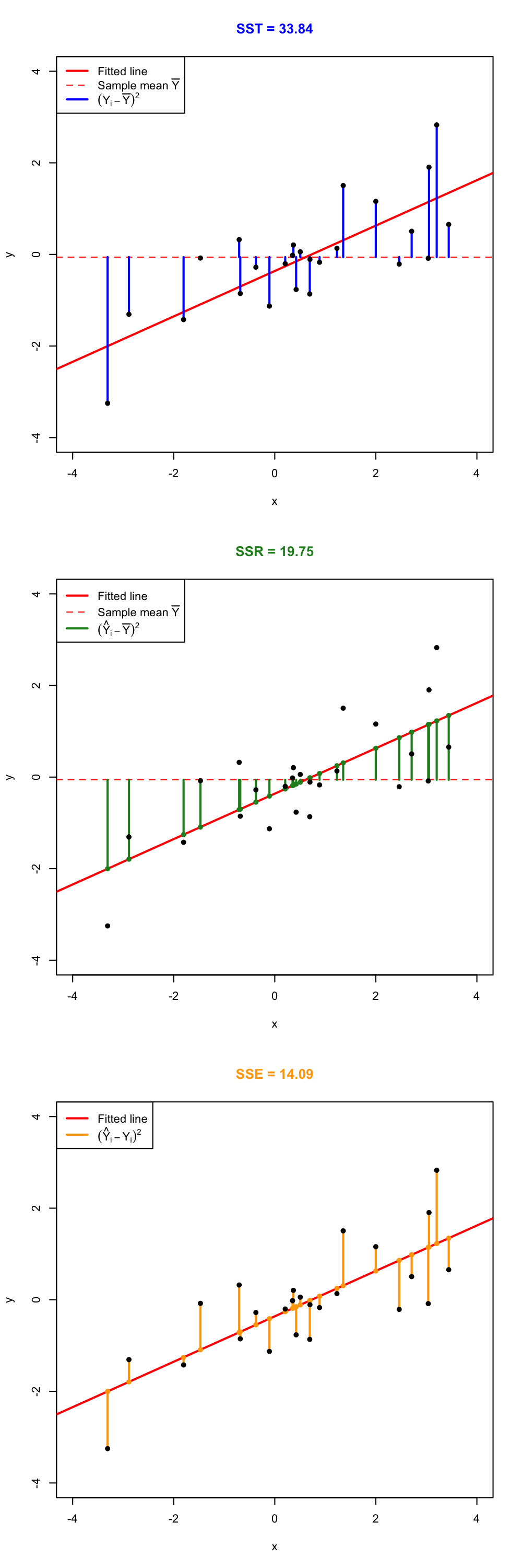
Figure 2.16: Visualization of the ANOVA decomposition. SST measures the variation of \(Y_1,\ldots,Y_n\) with respect to \(\bar Y.\) SSR measures the variation of \(\hat Y_1,\ldots,\hat Y_n\) with respect to \(\bar{\hat Y} = \bar Y.\) SSE collects the variation between \(Y_1,\ldots,Y_n\) and \(\hat Y_1,\ldots,\hat Y_n,\) that is, the variation of the residuals.

Figure 2.17: Illustration of the ANOVA decomposition and its dependence on \(\sigma^2\) and \(\hat\sigma^2.\) Larger (respectively, smaller) \(\hat\sigma^2\) results in more weight placed on the SSE (SSR) term. Application available here.

The “ANOVA table” is a broad concept in statistics, with different variants. Here we are only covering the basic ANOVA table from the relation \(\text{SST} = \text{SSR} + \text{SSE}.\) However, further sophistication is possible when \(\text{SSR}\) is decomposed into the variations contributed by each predictor. In particular, for multiple linear regression R’s anova implements a sequential (type I) ANOVA table, which is not the previous table!

The anova function takes a model as an input and returns the following sequential ANOVA table:⁴⁴

	Degrees of freedom	Sum Squares	Mean Squares	\(F\)-value	\(p\)-value
Predictor 1	\(1\)	SSR\(_1\)	\(\frac{\text{SSR}_1}{1}\)	\(\frac{\text{SSR}_1/1}{\text{SSE}/(n-p-1)}\)	\(p_1\)
Predictor 2	\(1\)	SSR\(_2\)	\(\frac{\text{SSR}_2}{1}\)	\(\frac{\text{SSR}_2/1}{\text{SSE}/(n-p-1)}\)	\(p_2\)
\(\vdots\)	\(\vdots\)	\(\vdots\)	\(\vdots\)	\(\vdots\)	\(\vdots\)
Predictor \(p\)	\(1\)	SSR\(_p\)	\(\frac{\text{SSR}_p}{1}\)	\(\frac{\text{SSR}_p/1}{\text{SSE}/(n-p-1)}\)	\(p_p\)
Residuals	\(n - p - 1\)	SSE	\(\frac{\text{SSE}}{n-p-1}\)

Here the \(\text{SSR}_j\) represents the regression sum of squares associated to the inclusion of \(X_j\) in the model with predictors \(X_1,\ldots,X_{j-1},\) that is:

\[\begin{align*} \text{SSR}_j=\text{SSR}(X_1,\ldots,X_j)-\text{SSR}(X_1,\ldots,X_{j-1}). \end{align*}\]

The \(p\)-values \(p_j\), \(j=1,\ldots,p,\) test the extra contribution of \(X_j\) when it is added after \(X_1,\ldots,X_{j-1}\). They do so by testing whether \(\text{SSR}_j\) is large relative to the \(\text{SSE}\) of the full model. These are a type of sequential, order-dependent \(F\)-tests. In general, they are not the same as the usual \(t\)-test for \(\beta_j\) in the model with predictors \(X_1,\ldots,X_j.\)

In order to exactly⁴⁵ compute the simplified ANOVA table seen before, we can rely on the following ad-hoc function. The function takes as input a fitted lm:

# This function computes the simplified anova from a linear model
simpleAnova <- function(object, ...) {

  # Compute anova table
  tab <- anova(object, ...)

  # Obtain number of predictors
  p <- nrow(tab) - 1

  # Add predictors row
  predictorsRow <- colSums(tab[1:p, 1:2])
  predictorsRow <- c(predictorsRow, predictorsRow[2] / predictorsRow[1])

  # F-quantities
  Fval <- predictorsRow[3] / tab[p + 1, 3]
  pval <- pf(Fval, df1 = p, df2 = tab$Df[p + 1], lower.tail = FALSE)
  predictorsRow <- c(predictorsRow, Fval, pval)

  # Simplified table
  tab <- rbind(predictorsRow, tab[p + 1, ])
  row.names(tab)[1] <- "Predictors"
  return(tab)

}

2.6.1 Case study application

Let’s compute the ANOVA decomposition of modWine1 and modWine2 to test the existence of linear dependence.

# Models
modWine1 <- lm(Price ~ ., data = wine)
modWine2 <- lm(Price ~ . - FrancePop, data = wine)

# Simplified table
simpleAnova(modWine1)
## Analysis of Variance Table
## 
## Response: Price
##            Df Sum Sq Mean Sq F value    Pr(>F)    
## Predictors  5 8.6671 1.73343  20.188 2.232e-07 ***
## Residuals  21 1.8032 0.08587                      
## ---
## Signif. codes:  0 '***' 0.001 '**' 0.01 '*' 0.05 '.' 0.1 ' ' 1
simpleAnova(modWine2)
## Analysis of Variance Table
## 
## Response: Price
##            Df Sum Sq Mean Sq F value    Pr(>F)    
## Predictors  4 8.6645 2.16613   26.39 4.057e-08 ***
## Residuals  22 1.8058 0.08208                      
## ---
## Signif. codes:  0 '***' 0.001 '**' 0.01 '*' 0.05 '.' 0.1 ' ' 1
# The null hypothesis of no linear dependence is emphatically rejected in
# both models

# R's ANOVA table -- warning this is not what we saw in lessons
anova(modWine1)
## Analysis of Variance Table
## 
## Response: Price
##             Df Sum Sq Mean Sq F value    Pr(>F)    
## WinterRain   1 0.1905  0.1905  2.2184 0.1512427    
## AGST         1 5.8989  5.8989 68.6990 4.645e-08 ***
## HarvestRain  1 1.6662  1.6662 19.4051 0.0002466 ***
## Age          1 0.9089  0.9089 10.5852 0.0038004 ** 
## FrancePop    1 0.0026  0.0026  0.0305 0.8631279    
## Residuals   21 1.8032  0.0859                      
## ---
## Signif. codes:  0 '***' 0.001 '**' 0.01 '*' 0.05 '.' 0.1 ' ' 1

Exercise 2.9 Compute the ANOVA table for the regression Price ~ WinterRain + AGST + HarvestRain + Age in the wine dataset. Check that the \(p\)-value for the \(F\)-test given in summary and by simpleAnova are the same.

Exercise 2.10 For the y6 ~ x6 and y7 ~ x7 in the assumptions dataset, compute their ANOVA tables. Check that the \(p\)-values of the \(t\)-test for \(\beta_1\) and the \(F\)-test are the same (any explanation of why this is so?).

2.7 Model fit

2.7.1 The \(R^2\)

The coefficient of determination \(R^2\) is closely related to the ANOVA decomposition. It is defined as

\[\begin{align} R^2:=\frac{\text{SSR}}{\text{SST}}=\frac{\text{SSR}}{\text{SSR}+\text{SSE}}=\frac{\text{SSR}}{\text{SSR}+(n-p-1)\hat\sigma^2}. \tag{2.21} \end{align}\]

The \(R^2\) measures the proportion of variation of the response variable \(Y\) that is explained by the predictors \(X_1,\ldots,X_p\) through the regression. Intuitively, \(R^2\) measures the tightness of the data cloud around the regression plane. Check in Figure 2.17 how the value of \(\sigma^2\)⁴⁶ affects the \(R^2.\)

The sample correlation coefficient is intimately related with the \(R^2.\) For example, if \(p=1,\) then it can be seen (exercise below) that \(R^2=r^2_{xy}.\) More importantly, \(R^2=r^2_{y\hat y}\) for any \(p,\) that is, the square of the sample correlation coefficient between \(Y_1,\ldots,Y_n\) and \(\hat Y_1,\ldots,\hat Y_n\) is \(R^2,\) a fact that is not immediately evident. Let’s check this fact when \(p=1\) by relying on \(R^2=r^2_{xy}.\) First, by the form of \(\hat\beta_0\) given in (2.3),

\[\begin{align} \hat Y_i&=\hat\beta_0+\hat\beta_1X_i\nonumber\\ &=(\bar Y-\hat\beta_1\bar X)+\hat\beta_1X_i\nonumber\\ &=\bar Y+\hat\beta_1(X_i-\bar X). \tag{2.22} \end{align}\]

Then, replace (2.22) in

\[\begin{align*} r^2_{y\hat y}&=\frac{s_{y\hat y}^2}{s_y^2s_{\hat y}^2}\\ &=\frac{\left(\sum_{i=1}^n \big(Y_i-\bar Y \big)\big(\hat Y_i-\bar Y \big)\right)^2}{\sum_{i=1}^n \big(Y_i-\bar Y \big)^2\sum_{i=1}^n \big(\hat Y_i-\bar Y \big)^2}\\ &=\frac{\left(\sum_{i=1}^n \big(Y_i-\bar Y \big)\big(\bar Y+\hat\beta_1(X_i-\bar X)-\bar Y \big)\right)^2}{\sum_{i=1}^n \big(Y_i-\bar Y \big)^2\sum_{i=1}^n \big(\bar Y+\hat\beta_1(X_i-\bar X)-\bar Y \big)^2}\\ &=r^2_{xy}. \end{align*}\]

As a consequence, \(r^2_{y\hat y}=r^2_{xy}=R^2\) when \(p=1.\)

Exercise 2.11 Show that \(R^2=r^2_{xy}\) when \(p=1.\) Hint: start from the definition of \(R^2\) and use (2.3) to arrive to \(r^2_{xy}.\)

Trusting the \(R^2\) blindly can lead to catastrophic conclusions. Here are a couple of counterexamples of a linear regression performed in a data that clearly does not satisfy the assumptions discussed in Section 2.3 but, despite that, the linear models have large \(R^2\)’s. These counterexamples emphasize that inference, built on the validity of the model assumptions,⁴⁷ will be problematic if these assumptions are violated, no matter what is the value of \(R^2.\) For example, recall how biased the predictions and their associated CIs will be in \(x=0.35\) and \(x=0.65.\)

# Simple linear model

# Create data that:
# 1) does not follow a linear model
# 2) the error is heteroscedastic
x <- seq(0.15, 1, l = 100)
set.seed(123456)
eps <- rnorm(n = 100, sd = 0.25 * x^2)
y <- 1 - 2 * x * (1 + 0.25 * sin(4 * pi * x)) + eps

# Great R^2!?
reg <- lm(y ~ x)
summary(reg)
## 
## Call:
## lm(formula = y ~ x)
## 
## Residuals:
##      Min       1Q   Median       3Q      Max 
## -0.53525 -0.18020  0.02811  0.16882  0.46896 
## 
## Coefficients:
##             Estimate Std. Error t value Pr(>|t|)    
## (Intercept)  0.87190    0.05860   14.88   <2e-16 ***
## x           -1.69268    0.09359  -18.09   <2e-16 ***
## ---
## Signif. codes:  0 '***' 0.001 '**' 0.01 '*' 0.05 '.' 0.1 ' ' 1
## 
## Residual standard error: 0.232 on 98 degrees of freedom
## Multiple R-squared:  0.7695, Adjusted R-squared:  0.7671 
## F-statistic: 327.1 on 1 and 98 DF,  p-value: < 2.2e-16

# scatterplot is a quick alternative to
# plot(x, y)
# abline(coef = reg$coef, col = 3)

# But prediction is obviously problematic
car::scatterplot(y ~ x, col = 1, regLine = list(col = 2), smooth = FALSE)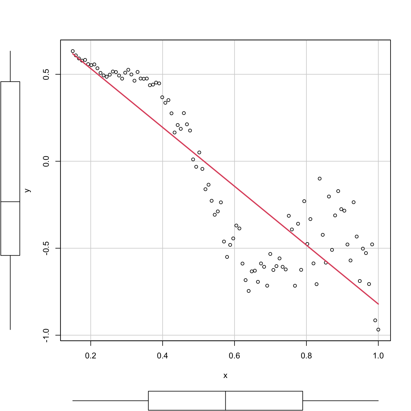

Figure 2.18: Regression line for a dataset that clearly violates the linearity and homoscedasticity assumptions. The \(R^2\) is, nevertheless, as high as (approximately) \(0.77.\)

# Multiple linear model

# Create data that:
# 1) does not follow a linear model
# 2) the error is heteroscedastic
x1 <- seq(0.15, 1, l = 100)
set.seed(123456)
x2 <- runif(100, -3, 3)
eps <- rnorm(n = 100, sd = 0.25 * x1^2)
y <- 1 - 3 * x1 * (1 + 0.25 * sin(4 * pi * x1)) + 0.25 * cos(x2) + eps

# Great R^2!?
reg <- lm(y ~ x1 + x2)
summary(reg)
## 
## Call:
## lm(formula = y ~ x1 + x2)
## 
## Residuals:
##      Min       1Q   Median       3Q      Max 
## -0.78737 -0.20946  0.01031  0.19652  1.05351 
## 
## Coefficients:
##              Estimate Std. Error t value Pr(>|t|)    
## (Intercept)  0.788812   0.096418   8.181  1.1e-12 ***
## x1          -2.540073   0.154876 -16.401  < 2e-16 ***
## x2           0.002283   0.020954   0.109    0.913    
## ---
## Signif. codes:  0 '***' 0.001 '**' 0.01 '*' 0.05 '.' 0.1 ' ' 1
## 
## Residual standard error: 0.3754 on 97 degrees of freedom
## Multiple R-squared:  0.744,  Adjusted R-squared:  0.7388 
## F-statistic:   141 on 2 and 97 DF,  p-value: < 2.2e-16

We can visualize the fit of the latter multiple linear model, since we are in \(p=2.\)

# But prediction is obviously problematic
car::scatter3d(y ~ x1 + x2, fit = "linear")
rgl::rglwidget()

The previous counterexamples illustrate that a large \(R^2\) means nothing in terms of inference if the assumptions of the model do not hold.

Remember that:

• \(R^2\) does not measure the correctness of a linear model but its usefulness, assuming the model is correct.
• \(R^2\) is the proportion of variance of \(Y\) explained by \(X_1,\ldots,X_p\) but, of course, only when the linear model is correct.

We finalize by pointing out a nice connection between the \(R^2,\) the ANOVA decomposition, and the least squares estimator \(\hat{\boldsymbol{\beta}}.\)

The ANOVA decomposition gives another view on the least-squares estimates: \(\hat{\boldsymbol{\beta}}\) are the estimated coefficients that maximize the \(R^2\) (among all the possible estimates we could think about). To see this, recall that

\[\begin{align*} R^2=\frac{\text{SSR}}{\text{SST}}=\frac{\text{SST} - \text{SSE}}{\text{SST}}=\frac{\text{SST} - \text{RSS}(\hat{\boldsymbol{\beta}})}{\text{SST}}. \end{align*}\]

Then, if \(\text{RSS}(\hat{\boldsymbol{\beta}})=\min_{\boldsymbol{\beta}\in\mathbb{R}^{p+1}}\text{RSS}(\boldsymbol{\beta}),\) then \(R^2\) is maximal for \(\hat{\boldsymbol{\beta}}.\)

2.7.2 The \(R^2\!{}_{\text{Adj}}\)

As we saw, these are equivalent forms for \(R^2\):

\[\begin{align} R^2=&\,\frac{\text{SSR}}{\text{SST}}=\frac{\text{SST}-\text{SSE}}{\text{SST}}=1-\frac{\text{SSE}}{\text{SST}}\nonumber\\ =&\,1-\frac{\hat\sigma^2}{\text{SST}}\times(n-p-1).\tag{2.23} \end{align}\]

The SSE on the numerator always decreases as more predictors are added to the model, even if these are not significant. As a consequence, the \(R^2\) always increases with \(p\). Why is this so? Intuitively, because the complexity – hence the flexibility – of the model increases when we use more predictors to explain \(Y.\) Mathematically, because when \(p\) approaches \(n-1\) the second term in (2.23) is reduced and, as a consequence, \(R^2\) grows.

The adjusted \(R^2\), \(R^2_\text{Adj},\) is an important quantity specifically designed to overcome this \(R^2\)’s flaw, ubiquitous in multiple linear regression. The purpose is to have a better tool for comparing models without systematically favoring more complex models.⁴⁸ This alternative coefficient is defined as

\[\begin{align} R^2_{\text{Adj}}:=&\,1-\frac{\text{SSE}/(n-p-1)}{\text{SST}/(n-1)}=1-\frac{\text{SSE}}{\text{SST}}\times\frac{n-1}{n-p-1}\nonumber\\ =&\,1-\frac{\hat\sigma^2}{\text{SST}}\times (n-1).\tag{2.24} \end{align}\]

The \(R^2_{\text{Adj}}\) is independent of \(p,\) at least explicitly. If \(p=1\) then \(R^2_{\text{Adj}}\) is almost \(R^2\) (practically identical if \(n\) is large). Both (2.23) and (2.24) are quite similar except for the last factor, which in the latter does not depend on \(p.\) Therefore, (2.24) will only increase if \(\hat\sigma^2\) is reduced with \(p;\) in other words, if the new variables contribute in the reduction of variability around the regression plane.

The different behavior between \(R^2\) and \(R^2_\text{Adj}\) can be visualized with the following simulation study. Suppose that we generate a random dataset \(\{(X_{i1},X_{i2},Y_i)\}_{i=1}^n,\) with \(n=200\) observations of two predictors \(X_1\) and \(X_2\) that are distributed as a \(\mathcal{N}(0,1),\) and a response \(Y\) generated by the linear model

\[\begin{align} Y_i=\beta_0+\beta_1X_{i1}+\beta_2X_{i2}+\varepsilon_i,\tag{2.25} \end{align}\]

where \(\varepsilon_i\sim\mathcal{N}(0,9).\) To this data, we add \(196\) “garbage” predictors \(X_j\sim\mathcal{N}(0,1)\) that are completely independent from \(Y.\) Therefore, we end up with \(p=198\) predictors where only the first two ones are relevant for explaining \(Y.\) We compute now the \(R^2(j)\) and \(R^2_\text{Adj}(j)\) for the models

\[\begin{align} Y=\beta_0+\beta_1X_{1}+\cdots+\beta_jX_{j}+\varepsilon,\tag{2.26} \end{align}\]

with \(j=1,\ldots,p,\) and we plot them as the curves \((j,R^2(j))\) and \((j,R_\text{Adj}^2(j)).\) Since \(R^2\) and \(R^2_\text{Adj}\) are random variables, we repeat this procedure \(M=500\) times to have an idea of the variability behind \(R^2\) and \(R^2_\text{Adj}.\) Figure 2.19 contains the results of this experiment.

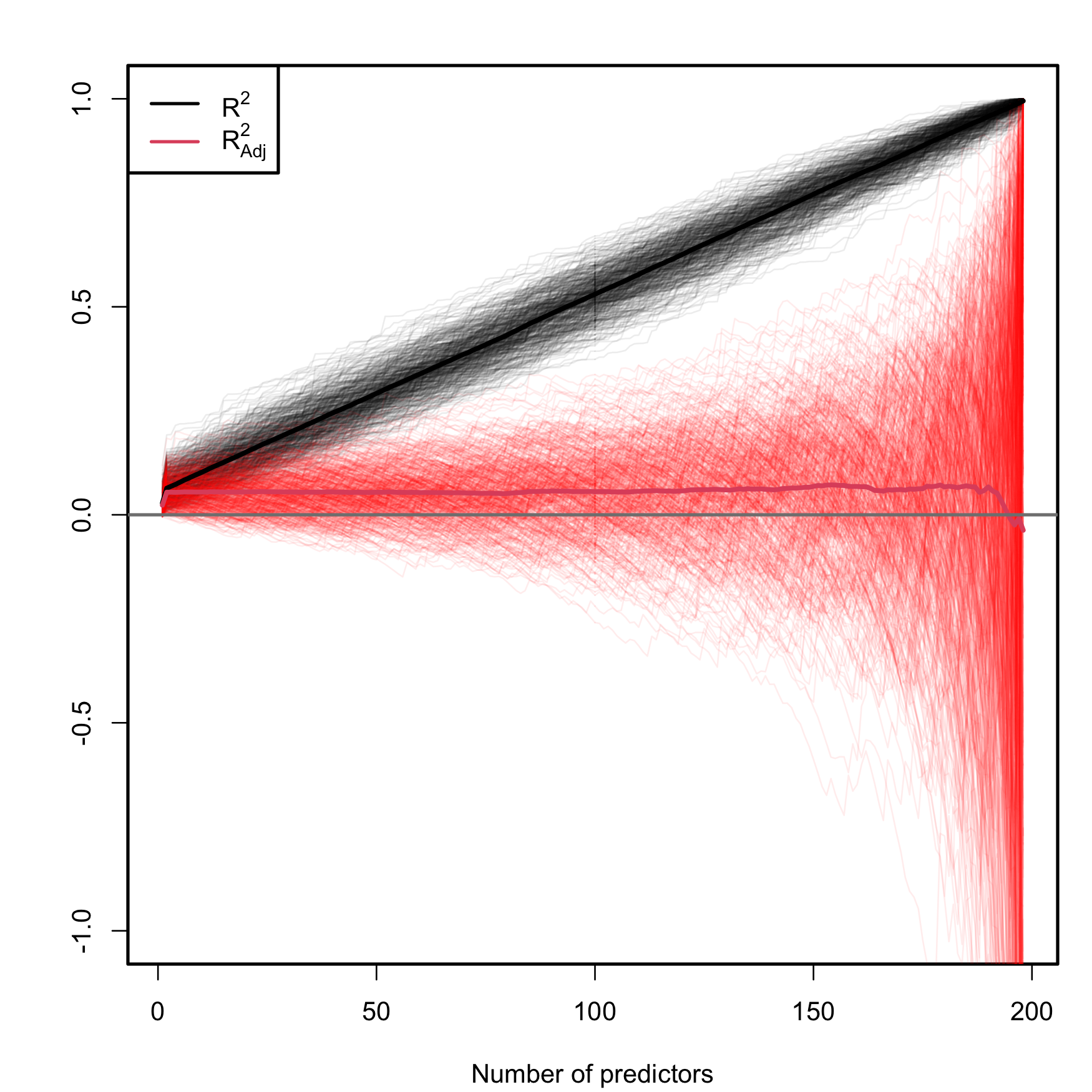
Figure 2.19: Comparison of \(R^2\) and \(R^2_{\text{Adj}}\) on the model (2.26) fitted with data generated by (2.25). The number of predictors \(p\) ranges from \(1\) to \(198,\) with only the first two predictors being significant. The \(M=500\) curves for each color arise from \(M\) simulated datasets of sample size \(n=200.\) The thicker curves are the mean of each color’s curves.

As it can be seen, the \(R^2\) increases linearly with the number of predictors considered, although only the first two ones were actually relevant. Thus, if we did not know about the random mechanism (2.25) that generated \(Y,\) we would be tempted to believe that the more adequate models would be the ones with a larger number of predictors. On the contrary, \(R^2_\text{Adj}\) only increases in the first two variables and then exhibits a mild decaying trend, indicating that, on average, the best choice for the number of predictors is actually close to \(p=2.\) However, note that \(R^2_\text{Adj}\) has a huge variability when \(p\) approaches \(n-2,\) a consequence of the explosive variance of \(\hat\sigma^2\) in that degenerate case⁴⁹. The experiment helps to visualize that \(R^2_\text{Adj}\) is more adequate than the \(R^2\) for evaluating the fit of a multiple linear regression⁵⁰.

An example of a simulated dataset considered in the experiment of Figure 2.19 is:

# Generate data
p <- 198
n <- 200
set.seed(3456732)
beta <- c(0.5, -0.5, rep(0, p - 2))
X <- matrix(rnorm(n * p), nrow = n, ncol = p)
Y <- drop(X %*% beta + rnorm(n, sd = 3))
data <- data.frame(y = Y, x = X)

# Regression on the two meaningful predictors
summary(lm(y ~ x.1 + x.2, data = data))

# Adding 20 "garbage" variables
# R^2 increases and adjusted R^2 decreases
summary(lm(y ~ X[, 1:22], data = data))

Exercise 2.12 Implement the simulation study behind Figure 2.19 in order to replicate it.

The \(R^2_\text{Adj}\) no longer measures the proportion of variation of \(Y\) explained by the regression, but the result of correcting this proportion by the number of predictors employed. As a consequence of this, \(R^2_\text{Adj}\leq1\) and \(R^2_\text{Adj}\) can be negative.

The next code illustrates a situation where we have two predictors completely independent from the response. The fitted model has a negative \(R^2_\text{Adj}.\)

# Three independent variables
set.seed(234599)
x1 <- rnorm(100)
x2 <- rnorm(100)
y <- 1 + rnorm(100)

# Negative adjusted R^2
summary(lm(y ~ x1 + x2))
## 
## Call:
## lm(formula = y ~ x1 + x2)
## 
## Residuals:
##     Min      1Q  Median      3Q     Max 
## -3.5081 -0.5021 -0.0191  0.5286  2.4750 
## 
## Coefficients:
##             Estimate Std. Error t value Pr(>|t|)    
## (Intercept)  0.97024    0.10399   9.330 3.75e-15 ***
## x1           0.09003    0.10300   0.874    0.384    
## x2          -0.05253    0.11090  -0.474    0.637    
## ---
## Signif. codes:  0 '***' 0.001 '**' 0.01 '*' 0.05 '.' 0.1 ' ' 1
## 
## Residual standard error: 1.034 on 97 degrees of freedom
## Multiple R-squared:  0.009797,   Adjusted R-squared:  -0.01062 
## F-statistic: 0.4799 on 2 and 97 DF,  p-value: 0.6203

Exercise 2.13 For the previous example, construct more predictors (x3, x4, …) that are independent from y. Then check that, when the predictors are added to the model, the \(R^2_\text{Adj}\) decreases and the \(R^2\) increases.

Beware of the \(R^2\) and \(R^2_\text{Adj}\) for model fits with no intercept! If the linear model is fitted with no intercept, the summary function silently returns a ‘Multiple R-squared’ and an ‘Adjusted R-squared’ that do not correspond (see this question in the R FAQ) with the seen expressions

\[\begin{align*} R^2=1-\frac{\text{SSE}}{\sum_{i=1}^n(Y_i-\bar{Y})^2},\quad R^2_{\text{Adj}}=1-\frac{\text{SSE}}{\text{SST}}\times\frac{n-1}{n-p-1}. \end{align*}\]

In the case with no intercept, summary rather returns

\[\begin{align*} R^2_0 :=1-\frac{\text{SSE}}{\sum_{i=1}^nY_i^2},\quad R^2_{0,\text{Adj}} :=1-\frac{\text{SSE}}{\sum_{i=1}^nY_i^2}\times\frac{n-1}{n-p-1}. \end{align*}\]

The reason is perhaps shocking: if the model is fitted without intercept and neither the response nor the predictors are centered, then the ANOVA decomposition does not hold, in the sense that

\[\begin{align*} \mathrm{SST} \neq \mathrm{SSR} + \mathrm{SSE}. \end{align*}\]

The fact that the ANOVA decomposition does not hold for no-intercept models has serious consequences on the theory we built. In particular, the \(R^2\) can be negative and \(R^2\neq r^2_{y\hat y},\) both deriving from the fact that \(\sum_{i=1}^n\hat\varepsilon_i\neq0.\) Therefore, the \(R^2\) cannot be regarded as the “proportion of variance explained” if the model fit is performed without intercept. The \(R^2_0\) and \(R^2_{0,\text{Adj}}\) versions are considered because they are the ones that arise from the “no-intercept ANOVA decomposition”

\[\begin{align*} \mathrm{SST}_0 = \mathrm{SSR}_0 + \mathrm{SSE},\quad \mathrm{SST}_0:=\sum_{i=1}^nY_i^2,\quad \mathrm{SSR}_0:=\sum_{i=1}^n\hat{Y}_i^2. \end{align*}\]

and therefore the \(R^2_0\) is guaranteed to be a quantity in \([0,1].\) It would indeed be the proportion of variance explained if the predictors and the response were centered (i.e., if \(\bar Y=0\) and \(\bar X_j=0,\) \(j=1,\ldots,p\)).

The next chunk of code illustrates these concepts for the iris dataset.

# Model with intercept
mod1 <- lm(Sepal.Length ~ Petal.Width, data = iris)
mod1
## 
## Call:
## lm(formula = Sepal.Length ~ Petal.Width, data = iris)
## 
## Coefficients:
## (Intercept)  Petal.Width  
##      4.7776       0.8886

# Model without intercept
mod0 <- lm(Sepal.Length ~ 0 + Petal.Width, data = iris)
mod0
## 
## Call:
## lm(formula = Sepal.Length ~ 0 + Petal.Width, data = iris)
## 
## Coefficients:
## Petal.Width  
##       3.731

# Recall the different way of obtaining the estimators
X1 <- cbind(1, iris$Petal.Width)
X0 <- cbind(iris$Petal.Width) # No column of ones!
Y <- iris$Sepal.Length
betaHat1 <- solve(crossprod(X1)) %*% t(X1) %*% Y
betaHat0 <- solve(crossprod(X0)) %*% t(X0) %*% Y
betaHat1
##           [,1]
## [1,] 4.7776294
## [2,] 0.8885803
betaHat0
##          [,1]
## [1,] 3.731485

# Summaries: higher R^2 for the model with no intercept!?
summary(mod1)
## 
## Call:
## lm(formula = Sepal.Length ~ Petal.Width, data = iris)
## 
## Residuals:
##      Min       1Q   Median       3Q      Max 
## -1.38822 -0.29358 -0.04393  0.26429  1.34521 
## 
## Coefficients:
##             Estimate Std. Error t value Pr(>|t|)    
## (Intercept)  4.77763    0.07293   65.51   <2e-16 ***
## Petal.Width  0.88858    0.05137   17.30   <2e-16 ***
## ---
## Signif. codes:  0 '***' 0.001 '**' 0.01 '*' 0.05 '.' 0.1 ' ' 1
## 
## Residual standard error: 0.478 on 148 degrees of freedom
## Multiple R-squared:  0.669,  Adjusted R-squared:  0.6668 
## F-statistic: 299.2 on 1 and 148 DF,  p-value: < 2.2e-16
summary(mod0)
## 
## Call:
## lm(formula = Sepal.Length ~ 0 + Petal.Width, data = iris)
## 
## Residuals:
##     Min      1Q  Median      3Q     Max 
## -3.1556 -0.3917  1.0625  3.8537  5.0537 
## 
## Coefficients:
##             Estimate Std. Error t value Pr(>|t|)    
## Petal.Width    3.732      0.150   24.87   <2e-16 ***
## ---
## Signif. codes:  0 '***' 0.001 '**' 0.01 '*' 0.05 '.' 0.1 ' ' 1
## 
## Residual standard error: 2.609 on 149 degrees of freedom
## Multiple R-squared:  0.8058, Adjusted R-squared:  0.8045 
## F-statistic: 618.4 on 1 and 149 DF,  p-value: < 2.2e-16

# Wait a moment... let's see the actual fit
plot(Sepal.Length ~ Petal.Width, data = iris)
abline(mod1, col = 2) # Obviously, much better
abline(mod0, col = 3)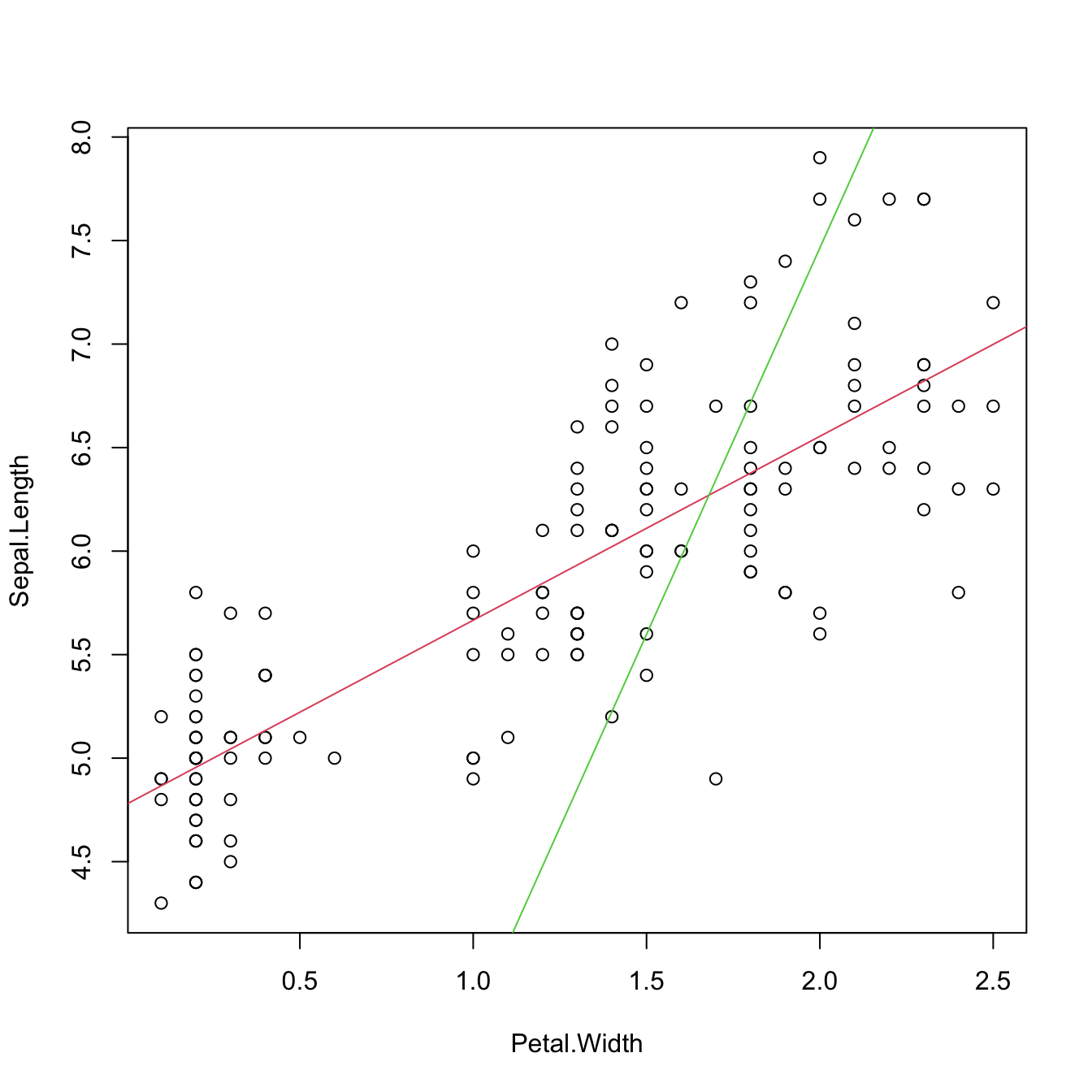

# Compute the R^2 manually for mod1
SSE1 <- sum(mod1$residuals^2)
SST1 <- sum((mod1$model$Sepal.Length - mean(mod1$model$Sepal.Length))^2)
1 - SSE1 / SST1
## [1] 0.6690277

# Compute the R^2 manually for mod0
SSE0 <- sum(mod0$residuals^2)
SST0 <- sum((mod0$model$Sepal.Length - mean(mod0$model$Sepal.Length))^2)
1 - SSE0 / SST0
## [1] -8.926872
# It is negative!

# Recall that the mean of the residuals is not zero!
mean(mod0$residuals)
## [1] 1.368038

# What summary really returns if there is no intercept
n <- nrow(iris)
p <- 1
R0 <- 1 - sum(mod0$residuals^2) / sum(mod0$model$Sepal.Length^2)
R0Adj <- 1 - sum(mod0$residuals^2) / sum(mod0$model$Sepal.Length^2) *
  (n - 1) / (n - p - 1)
R0
## [1] 0.8058497
R0Adj
## [1] 0.8045379

# What if we centered the data previously?
irisCen <- data.frame(scale(iris[, -5], center = TRUE, scale = FALSE))
modCen1 <- lm(Sepal.Length ~ Petal.Width, data = irisCen)
modCen0 <- lm(Sepal.Length ~ 0 + Petal.Width, data = irisCen)

# No problem, "correct" R^2
summary(modCen1)
## 
## Call:
## lm(formula = Sepal.Length ~ Petal.Width, data = irisCen)
## 
## Residuals:
##      Min       1Q   Median       3Q      Max 
## -1.38822 -0.29358 -0.04393  0.26429  1.34521 
## 
## Coefficients:
##               Estimate Std. Error t value Pr(>|t|)    
## (Intercept) -9.050e-16  3.903e-02     0.0        1    
## Petal.Width  8.886e-01  5.137e-02    17.3   <2e-16 ***
## ---
## Signif. codes:  0 '***' 0.001 '**' 0.01 '*' 0.05 '.' 0.1 ' ' 1
## 
## Residual standard error: 0.478 on 148 degrees of freedom
## Multiple R-squared:  0.669,  Adjusted R-squared:  0.6668 
## F-statistic: 299.2 on 1 and 148 DF,  p-value: < 2.2e-16
summary(modCen0)
## 
## Call:
## lm(formula = Sepal.Length ~ 0 + Petal.Width, data = irisCen)
## 
## Residuals:
##      Min       1Q   Median       3Q      Max 
## -1.38822 -0.29358 -0.04393  0.26429  1.34521 
## 
## Coefficients:
##             Estimate Std. Error t value Pr(>|t|)    
## Petal.Width   0.8886     0.0512   17.36   <2e-16 ***
## ---
## Signif. codes:  0 '***' 0.001 '**' 0.01 '*' 0.05 '.' 0.1 ' ' 1
## 
## Residual standard error: 0.4764 on 149 degrees of freedom
## Multiple R-squared:  0.669,  Adjusted R-squared:  0.6668 
## F-statistic: 301.2 on 1 and 149 DF,  p-value: < 2.2e-16

# But only if we center predictor and response...
summary(lm(iris$Sepal.Length ~ 0 + irisCen$Petal.Width))
## 
## Call:
## lm(formula = iris$Sepal.Length ~ 0 + irisCen$Petal.Width)
## 
## Residuals:
##    Min     1Q Median     3Q    Max 
##  4.455  5.550  5.799  6.108  7.189 
## 
## Coefficients:
##                     Estimate Std. Error t value Pr(>|t|)
## irisCen$Petal.Width   0.8886     0.6322   1.406    0.162
## 
## Residual standard error: 5.882 on 149 degrees of freedom
## Multiple R-squared:  0.01308,    Adjusted R-squared:  0.006461 
## F-statistic: 1.975 on 1 and 149 DF,  p-value: 0.1619

Exercise 2.14 Let’s play the evil practitioner and try to modify the \(R_0^2\) returned by summary when the intercept is excluded. If we were really evil, we could use this knowledge to fool someone that is not aware of the difference between \(R_0^2\) and \(R^2\) into believing that any given model is incredibly good or bad in terms of the \(R^2\)!

1. For the previous example, display the \(R_0^2\) as a function of a shift in mean of the predictor Petal.Width. What can you conclude? Hint: you may use I() for performing the shifting inside the model equation.
2. What shift on Petal.Width would be necessary to achieve an \(R_0^2\approx0.95\)? Is this shift unique?
3. Do the same but for a shift in the mean of the response Sepal.Length. What shift would be necessary to achieve an \(R_0^2\approx0.50\)? Is there a single shift?
4. Consider the multiple linear model medv ~ nox + rm for the Boston dataset. We want to tweak the \(R_0^2\) to set it to any number in \([0,1].\) Can we achieve this by only shifting rm or medv (only one of them)?
5. Explore systematically the \(R_0^2\) for the shifting combinations of rm and medv and obtain a combination that delivers an \(R_0^2\approx 0.30.\) Hint: use filled.contour() for visualizing the \(R_0^2\) surface.

2.7.3 Case study application

Coming back to the case study, we have studied so far three models:

# Fit models
modWine1 <- lm(Price ~ ., data = wine)
modWine2 <- lm(Price ~ . - FrancePop, data = wine)
modWine3 <- lm(Price ~ Age + WinterRain, data = wine)

# Summaries
summary(modWine1)
## 
## Call:
## lm(formula = Price ~ ., data = wine)
## 
## Residuals:
##      Min       1Q   Median       3Q      Max 
## -0.46541 -0.24133  0.00413  0.18974  0.52495 
## 
## Coefficients:
##               Estimate Std. Error t value Pr(>|t|)    
## (Intercept) -2.343e+00  7.697e+00  -0.304  0.76384    
## WinterRain   1.153e-03  4.991e-04   2.311  0.03109 *  
## AGST         6.144e-01  9.799e-02   6.270 3.22e-06 ***
## HarvestRain -3.837e-03  8.366e-04  -4.587  0.00016 ***
## Age          1.377e-02  5.821e-02   0.237  0.81531    
## FrancePop   -2.213e-05  1.268e-04  -0.175  0.86313    
## ---
## Signif. codes:  0 '***' 0.001 '**' 0.01 '*' 0.05 '.' 0.1 ' ' 1
## 
## Residual standard error: 0.293 on 21 degrees of freedom
## Multiple R-squared:  0.8278, Adjusted R-squared:  0.7868 
## F-statistic: 20.19 on 5 and 21 DF,  p-value: 2.232e-07
summary(modWine2)
## 
## Call:
## lm(formula = Price ~ . - FrancePop, data = wine)
## 
## Residuals:
##      Min       1Q   Median       3Q      Max 
## -0.46024 -0.23862  0.01347  0.18601  0.53443 
## 
## Coefficients:
##               Estimate Std. Error t value Pr(>|t|)    
## (Intercept) -3.6515703  1.6880876  -2.163  0.04167 *  
## WinterRain   0.0011667  0.0004820   2.420  0.02421 *  
## AGST         0.6163916  0.0951747   6.476 1.63e-06 ***
## HarvestRain -0.0038606  0.0008075  -4.781 8.97e-05 ***
## Age          0.0238480  0.0071667   3.328  0.00305 ** 
## ---
## Signif. codes:  0 '***' 0.001 '**' 0.01 '*' 0.05 '.' 0.1 ' ' 1
## 
## Residual standard error: 0.2865 on 22 degrees of freedom
## Multiple R-squared:  0.8275, Adjusted R-squared:  0.7962 
## F-statistic: 26.39 on 4 and 22 DF,  p-value: 4.057e-08
summary(modWine3)
## 
## Call:
## lm(formula = Price ~ Age + WinterRain, data = wine)
## 
## Residuals:
##      Min       1Q   Median       3Q      Max 
## -0.88964 -0.51421 -0.00066  0.43103  1.06897 
## 
## Coefficients:
##              Estimate Std. Error t value Pr(>|t|)    
## (Intercept) 5.9830427  0.5993667   9.982 5.09e-10 ***
## Age         0.0360559  0.0137377   2.625   0.0149 *  
## WinterRain  0.0007813  0.0008780   0.890   0.3824    
## ---
## Signif. codes:  0 '***' 0.001 '**' 0.01 '*' 0.05 '.' 0.1 ' ' 1
## 
## Residual standard error: 0.5769 on 24 degrees of freedom
## Multiple R-squared:  0.2371, Adjusted R-squared:  0.1736 
## F-statistic:  3.73 on 2 and 24 DF,  p-value: 0.03884

The model modWine2 has the largest \(R^2_\text{Adj}\) among the three studied. It is a model that explains the \(82.75\%\) of the variability in a non-redundant way and with all its coefficients significant. Therefore, we have a formula for effectively explaining and predicting the quality of a vintage (answers Q1). Prediction and, importantly, quantification of the uncertainty in the prediction, can be done through the predict function.

Furthermore, the interpretation of modWine2 agrees with well-known facts in viticulture that make perfect sense. Precisely (answers Q2):

• Higher temperatures are associated with better quality (higher priced) wine.
• Rain before the growing season is good for the wine quality, but during harvest is bad.
• The quality of the wine improves with the age.

Although these conclusions could be regarded as common folklore, keep in mind that this model

• allows us to quantify the effect of each variable on the wine quality and
• provides a precise way of predicting the quality of future vintages.

References

Ashenfelter, O., D. Ashmore, and R. Lalonde. 1995. “Bordeaux Wine Vintage Quality and the Weather.” CHANCE 8 (4): 7–14. https://doi.org/10.1080/09332480.1995.10542468.

---

14. “How computers routed the experts”, Financial Times, 31/08/2007.↩︎

15. Young wines are astringent, when the wines age they lose their astringency.↩︎

16. Source: http://www.liquidasset.com/winedata.html.↩︎

17. They are unique and always exist (except if \(s_x=0,\) when all the data points are the same). They can be obtained by solving \(\frac{\partial}{\partial \beta_0}\text{RSS}(\beta_0,\beta_1)=0\) and \(\frac{\partial}{\partial \beta_1}\text{RSS}(\beta_0,\beta_1)=0.\)↩︎

18. The sample standard deviation is \(s_x=\sqrt{s_x^2}.\)↩︎

19. Note that now \(X_1\) represents the first predictor and not the first element of a sample of \(X.\)↩︎

20. Recall that (2.4) and (2.5) were referring to the relation of the random variable (or population) \(Y\) with the random variables \(X_1,\ldots,X_p.\) Those are population versions of the linear model and clearly generate the sample versions when they are replicated for each observation \((\mathbf{X}_{i},Y_i),\) \(i=1,\ldots,n,\) of the random vector \((\mathbf{X},Y).\)↩︎

21. It can be seen that they are unique and that they always exist, provided that \(\mathrm{rank}(\mathbf{X}^ op\mathbf{X})=p+1.\)↩︎

22. It follows from \(\frac{\partial (\mathbf{A}\mathbf{x})}{\partial \mathbf{x}}=\mathbf{A}\) and \(\frac{\partial (f(\mathbf{x})^\top g(\mathbf{x}))}{\partial \mathbf{x}}=f(\mathbf{x})^\top\frac{\partial g(\mathbf{x})}{\partial \mathbf{x}}+g(\mathbf{x})^\top\frac{\partial f(\mathbf{x})}{\partial \mathbf{x}}\) for two vector-valued functions \(f,g:\mathbb{R}^p\rightarrow \mathbb{R}^m,\) where \(\frac{\partial (f(\mathbf{x})^\top g(\mathbf{x}))}{\partial \mathbf{x}}\) is the gradient row vector of \(f^\top g,\) and \(\frac{\partial f(\mathbf{x})}{\partial \mathbf{x}}\) and \(\frac{\partial g(\mathbf{x})}{\partial \mathbf{x}}\) are the Jacobian matrices of \(f\) and \(g,\) respectively.↩︎

23. If you wanted to do so, you will need to use the function I() for indicating that + is not including predictors in the model, but is acting as the algebraic sum operator.↩︎

24. After all, we already have a neat way of estimating \(\boldsymbol{\beta}\) from the data… Isn’t that all that is needed?↩︎

25. This is for theoretical and modeling convenience. With this assumption, we just model the randomness of \(Y\) given the predictors. If the randomness of \(Y\) and the randomness of \(X_1,\ldots,X_n\) was to be modeled, we would require a significantly more complex model.↩︎

26. Understood as small \(|(\mathbf{X}^\top\mathbf{X})^{-1}|.\)↩︎

27. Prior to undertaking the estimation of \(\sigma\) we have used the sample to estimate \(\hat{\boldsymbol\beta}.\) The situation is thus analogous to the discussion between the sample variance \(s_x^2=\frac{1}{n}\sum_{i=1}^n\left(X_i-\bar{X}\right)^2\) and the sample quasi-variance \(\hat{s}_x^2=\frac{1}{n-1}\sum_{i=1}^n\left(X_i-\bar{X}\right)^2\) that are computed from a sample \(X_1,\ldots,X_n.\) When estimating \(\mathbb{V}\mathrm{ar}[X],\) both estimate previously \(\mathbb{E}[X]\) through \(\bar{X}.\) The fact that \(\hat{s}_x^2\) accounts for that prior estimation through the degrees of freedom \(n-1\) makes that estimator unbiased for \(\mathbb{V}\mathrm{ar}[X]\) (\(s_x^2\) is not).↩︎

28. Recall that the sample variance of \(\hat\varepsilon_1,\ldots,\hat\varepsilon_n\) is \(\frac{1}{n}\sum_{i=1}^n\left(\hat\varepsilon_i-\bar{\hat\varepsilon}\right)^2.\)↩︎

29. In the sense of practically realistic.↩︎

30. Shortcut for significantly different from zero.↩︎

31. This is denoted as \(\frac{\hat{\beta}_j-0}{\hat{\mathrm{SE}}(\hat\beta_j)}\stackrel{H_0}{\sim}t_{n-p-1}.\)↩︎

32. In R, \(t_{n-p-1;\alpha/2}\) can be computed as qt(p = 1 - alpha / 2, df = n - p - 1) or qt(p = alpha / 2, df = n - p - 1, lower.tail = FALSE).↩︎

33. For example, '**' indicates that the \(p\)-value lies within \(0.001\) and \(0.01.\)↩︎

34. This is a context-guided decision, not data-driven.↩︎

35. Notice the use of - for excluding a particular predictor.↩︎

36. Because the prediction of a new observation from the random variable \(\mathcal{N}(\beta_0+\beta_1x_1+\cdots+\beta_{p}x_p,\sigma^2)\) is simply its mean, \(\beta_0+\beta_1x_1+\cdots+\beta_{p}x_p,\) which is also the most likely value in a normal.↩︎

37. A consequence of this extra \(\hat\sigma^2\) is that the length of (2.19) cannot be reduced arbitrarily if the sample size \(n\) grows.↩︎

38. This is an important result that can be checked using the matrix notation introduced in Section 2.2.3.↩︎

39. Recall that SSE and RSS (of the least squares estimator \(\hat{\boldsymbol{\beta}}\)) are two names for the same quantity (that appears in different contexts): \(\text{SSE}=\sum_{i=1}^n\big(Y_i-\hat Y_i\big)^2=\sum_{i=1}^n\big(Y_i-\hat \beta_0-\hat \beta_1X_{i1}-\cdots-\hat \beta_pX_{ip}\big)^2=\mathrm{RSS}(\hat{\boldsymbol{\beta}}).\)↩︎

40. Geometrically: the plane is completely flat, it does not have any inclination in the \(Y\) direction.↩︎

41. And therefore, there is a statistical meaningful (i.e., not constant) linear trend to model.↩︎

42. Little variation is explained by the regression model since \(\hat{\boldsymbol{\beta}}\approx\mathbf{0}.\)↩︎

43. In R, qf(p = 1 - alpha, df1 = n - p - 1, df2 = p) or qf(p = alpha, df1 = n - p - 1, df2 = p, lower.tail = FALSE).↩︎

44. More complex – included here just for clarification of the anova’s output.↩︎

45. Note that, if mod <- lm(resp ~ preds, data) represents a model with response resp and predictors preds, and mod0, is the intercept-only model mod0 <- lm(resp ~ 1, data) that does not contain predictors, anova(mod0, mod) gives a similar, output to the seen ANOVA table. Precisely, the first row of the outputted table stands for the SST and the second row for the SSE row (so we call it the SST–SSE table). The SSR row is not present. The seen ANOVA table (which contains SSR and SSE) and the SST–SSE table encode the same information due to the ANOVA decomposition. So it is a matter of taste and tradition to employ one or the other. In particular, both have the \(F\)-test and its associated \(p\)-value (in the SSE row for the SST–SSE table).↩︎

46. Which is not the \(\hat\sigma^2\) in (2.21), but \(\hat\sigma^2\) is obviously dependent on \(\sigma^2.\)↩︎

47. Which do not hold!↩︎

48. An informal way of regarding the difference between \(R^2\) and \(R^2_\text{Adj}\) is by thinking of \(R^2\) as a measure of fit that “is not aware of the dangers of overfitting”. In this interpretation, \(R^2_\text{Adj}\) is the overfitting-aware version of \(R^2.\)↩︎

49. This indicates that \(R^2_\text{Adj}\) can act as a model selection device up to a certain point, as its effectiveness becomes too variable, too erratic, when the number of predictors is very high in comparison with \(n.\)↩︎

50. Coincidentally, the experiment also serves as a reminder about the randomness of \(R^2\) and \(R^2_{\text{Adj}},\) a fact that is sometimes overlooked.↩︎