6 Nonparametric regression

The models we saw in the previous chapters share a common root: all of them are parametric. This means that they assume a certain structure on the regression function $m,$ which is controlled by parameters.¹⁸⁸ If this assumption truly holds, then parametric methods are the best approach for estimating $m.$ But in practice it is rarely the case where parametric methods work out-of-the-box, and several tricks are needed in order to expand their degree of flexibility on a case-by-case basis. Avoiding this nuisance is the strongest point of nonparametric methods: they do not assume major hard-to-satisfy hypotheses on the regression function, but just minimal assumptions, which makes them directly employable. Their weak points are that they usually are more computationally demanding and are harder to interpret.

We consider first the simplest situation:¹⁸⁹ a single continuous predictor $X$ for predicting a response $Y.$ In this case, recall that the complete knowledge of $Y$ when $X=x$ is given by the conditional pdf $f_{Y \mid X=x}(y)=\frac{f(x,y)}{f_X(x)}.$ While this pdf provides full knowledge about $Y \mid X=x,$ it is also a challenging task to estimate it: for each $x$ we have to estimate a different curve! A simpler approach, yet still challenging, is to estimate the conditional mean (a scalar) for each $x$ through the regression function

\[\begin{align*} m(x)=\mathbb{E}[Y \mid X=x]=\int yf_{Y \mid X=x}(y)\,\mathrm{d}y. \end{align*}\]

As we will see, this density-based view of the regression function is useful in order to motivate estimators.

6.1 Nonparametric density estimation

In order to introduce a nonparametric estimator for the regression function $m,$ we need to introduce first a nonparametric estimator for the density of the predictor $X.$ This estimator is aimed to estimate $f,$ the density of $X,$ from a sample $X_1,\ldots,X_n$ without assuming any specific form for $f.$ That is, without assuming, e.g., that the data is normally distributed.

6.1.1 Histogram and moving histogram

The simplest method to estimate a density $f$ from an iid sample $X_1,\ldots,X_n$ is the histogram. From an analytical point of view, the idea is to aggregate the data in intervals of the form $[x_0,x_0+h)$ and then use their relative frequency to approximate the density at $x\in[x_0,x_0+h),$ $f(x),$ by the estimate of

\[\begin{align*} f(x_0)&=F'(x_0)\\ &=\lim_{h\to0^+}\frac{F(x_0+h)-F(x_0)}{h}\\ &=\lim_{h\to0^+}\frac{\mathbb{P}[x_0<X< x_0+h]}{h}. \end{align*}\]

More precisely, given an origin $t_0$ and a bandwidth $h>0,$ the histogram builds a piecewise constant function in the intervals $\{B_k:=[t_{k},t_{k+1}):t_k=t_0+hk,k\in\mathbb{Z}\}$ by counting the number of sample points inside each of them. These constant-length intervals are also called bins. The fact they have constant length $h$ is important, since it allows us to standardize by $h$ in order to have relative frequencies per length¹⁹⁰ in the bins. The histogram at a point $x$ is defined as

\[\begin{align} \hat{f}_\mathrm{H}(x;t_0,h):=\frac{1}{nh}\sum_{i=1}^n1_{\{X_i\in B_k:x\in B_k\}}. \tag{6.1} \end{align}\]

Equivalently, if we denote the number of points in $B_k$ as $v_k,$ then the histogram is $\hat{f}_\mathrm{H}(x;t_0,h)=\frac{v_k}{nh}$ if $x\in B_k$ for $k\in\mathbb{Z}.$

The computation of histograms is straightforward in R. As an example, we consider the faithful dataset, which contains the duration of the eruption and the waiting time between eruptions for the Old Faithful geyser in Yellowstone National Park (USA).

# Duration of eruption
faithE <- faithful$eruptions

# Default histogram: automatically chooses bins and uses absolute frequencies
histo <- hist(faithE)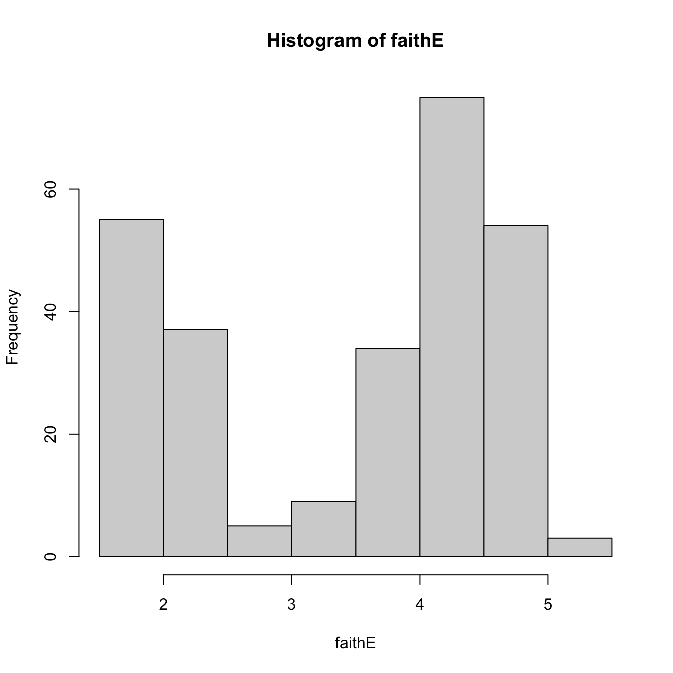


# Bins and bin counts
histo$breaks # Bk's
## [1] 1.5 2.0 2.5 3.0 3.5 4.0 4.5 5.0 5.5
histo$counts # vk's
## [1] 55 37  5  9 34 75 54  3

# With relative frequencies
hist(faithE, probability = TRUE)


# Choosing the breaks
t0 <- min(faithE)
h <- 0.25
Bk <- seq(t0, max(faithE), by = h)
hist(faithE, probability = TRUE, breaks = Bk)
rug(faithE) # The sample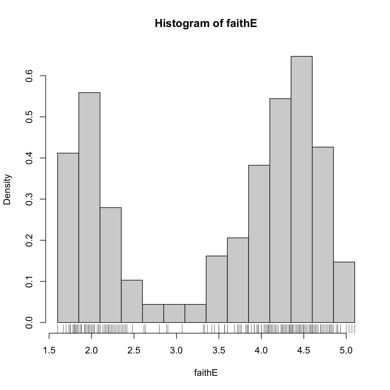

Recall that the shape of the histogram depends on:

$t_0,$ since the separation between bins happens at $t_0k,$ $k\in\mathbb{Z};$
$h,$ which controls the bin size and the effective number of bins for aggregating the sample.

We focus first on exploring the dependence on $t_0$ with the next example, as it serves for motivating the next density estimator.

# Uniform sample
set.seed(1234567)
u <- runif(n = 100)

# t0 = 0, h = 0.2
Bk1 <- seq(0, 1, by = 0.2)

# t0 = -0.1, h = 0.2
Bk2 <- seq(-0.1, 1.1, by = 0.2)

# Comparison
par(mfrow = 1:2)
hist(u, probability = TRUE, breaks = Bk1, ylim = c(0, 1.5),
     main = "t0 = 0, h = 0.2")
rug(u)
abline(h = 1, col = 2)
hist(u, probability = TRUE, breaks = Bk2, ylim = c(0, 1.5),
     main = "t0 = -0.1, h = 0.2")
rug(u)
abline(h = 1, col = 2)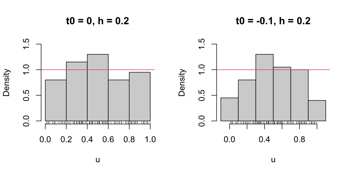

$The dependence of the histogram on the origin $t_0$.$

Figure 6.1: The dependence of the histogram on the origin $t_0$.

Clearly, this dependence is undesirable, as it is prone to change notably the estimation of $f$ using the same data. An alternative to avoid the dependence on $t_0$ is the moving histogram or naive density estimator. The idea is to aggregate the sample $X_1,\ldots,X_n$ in intervals of the form $(x-h, x+h)$ and then use its relative frequency in $(x-h,x+h)$ to approximate the density at $x,$ which can be written as

\[\begin{align*} f(x)&=F'(x)\\ &=\lim_{h\to0^+}\frac{F(x+h)-F(x-h)}{2h}\\ &=\lim_{h\to0^+}\frac{\mathbb{P}[x-h<X<x+h]}{2h}. \end{align*}\]

Recall the differences with the histogram: the intervals depend on the evaluation point $x$ and are centered about it. That allows to directly estimate $f(x)$ (without the proxy $f(x_0)$) by an estimate of the symmetric derivative.

Given a bandwidth $h>0,$ the naive density estimator builds a piecewise constant function by considering the relative frequency of $X_1,\ldots,X_n$ inside $(x-h,x+h)$:¹⁹¹

\[\begin{align} \hat{f}_\mathrm{N}(x;h):=\frac{1}{2nh}\sum_{i=1}^n1_{\{x-h<X_i<x+h\}}. \tag{6.2} \end{align}\]

The analysis of $\hat{f}_\mathrm{N}(x;h)$ as a random variable follows from realizing that

\[\begin{align*} \sum_{i=1}^n1_{\{x-h<X_i<x+h\}}\sim \mathrm{B}(n,p_{x,h}) \end{align*}\]

where

\[\begin{align*} p_{x,h}:=\mathbb{P}[x-h<X<x+h]=F(x+h)-F(x-h). \end{align*}\]

Therefore, employing the bias and variance expressions of a binomial,¹⁹² it follows:

\[\begin{align*} \mathbb{E}[\hat{f}_\mathrm{N}(x;h)]=&\,\frac{F(x+h)-F(x-h)}{2h},\\ \mathbb{V}\mathrm{ar}[\hat{f}_\mathrm{N}(x;h)]=&\,\frac{F(x+h)-F(x-h)}{4nh^2}\\ &-\frac{(F(x+h)-F(x-h))^2}{4nh^2}. \end{align*}\]

These two results provide very interesting insights on the effect of $h$ on the moving histogram:

If $h\to0,$ then $\mathbb{E}[\hat{f}_\mathrm{N}(x;h)]\to f(x)$ and (6.2) is an asymptotically unbiased estimator of $f(x).$ However, if $h\to0,$ the variance explodes: $\mathbb{V}\mathrm{ar}[\hat{f}_\mathrm{N}(x;h)]\approx \frac{f(x)}{2nh}-\frac{f(x)^2}{n}\to\infty.$
If $h\to\infty,$ then both $\mathbb{E}[\hat{f}_\mathrm{N}(x;h)]\to 0$ and $\mathbb{V}\mathrm{ar}[\hat{f}_\mathrm{N}(x;h)]\to0.$ Therefore, the variance shrinks to zero but the bias grows.
If $nh\to\infty,$¹⁹³ then the variance shrinks to zero. If, in addition, $h\to0,$ the bias also shrinks to zero. So both the bias and the variance are reduced if $n\to\infty,$ $h\to0,$ and $nh\to\infty,$ simultaneously.

The animation in Figure 6.2 illustrates the previous points and gives insight on how the performance of (6.2) varies with $h.$

Figure 6.2: Bias and variance for the moving histogram. The animation shows how for small bandwidths the bias of $\hat{f}_\mathrm{N}(x;h)$ on estimating $f(x)$ is small, but the variance is high, and how for large bandwidths the bias is large and the variance is small. The variance is represented by the asymptotic $95\%$ confidence intervals for $\hat{f}_\mathrm{N}(x;h).$ Recall how the variance of $\hat{f}_\mathrm{N}(x;h)$ is (almost) proportional to $f(x).$ Application also available here.

The estimator (6.2) poses an interesting question:

Why giving the same weight to all $X_1,\ldots,X_n$ in $(x-h, x+h)$ for estimating $f(x)$?

We are estimating $f(x)=F'(x)$ by estimating $\frac{F(x+h)-F(x-h)}{2h}$ through the relative frequency of $X_1,\ldots,X_n$ in the interval $(x-h,x+h).$ Should not the data points closer to $x$ be more important than the ones further away? The answer to this question shows that (6.2) is indeed a particular case of a wider class of density estimators.

6.1.2 Kernel density estimation

The moving histogram (6.2) can be equivalently written as

\[\begin{align} \hat{f}_\mathrm{N}(x;h)&=\frac{1}{nh}\sum_{i=1}^n\frac{1}{2}1_{\left\{-1<\frac{x-X_i}{h}<1\right\}}\nonumber\\ &=\frac{1}{nh}\sum_{i=1}^nK\left(\frac{x-X_i}{h}\right), \tag{6.3} \end{align}\]

with $K(z)=\frac{1}{2}1_{\{-1<z<1\}}.$ Interestingly, $K$ is a uniform density in $(-1,1).$ This means that, when approximating

\[\begin{align*} \mathbb{P}[x-h<X<x+h]=\mathbb{P}\left[-1<\frac{x-X}{h}<1\right] \end{align*}\]

by (6.3), we give equal weight to all the points $X_1,\ldots,X_n.$ The generalization of (6.3) is now obvious: replace $K$ by an arbitrary density. Then $K$ is known as a kernel: a density with certain regularity that is (typically) symmetric and unimodal at $0.$ This generalization provides the definition of kernel density estimator¹⁹⁴ (kde):

\[\begin{align} \hat{f}(x;h):=\frac{1}{nh}\sum_{i=1}^nK\left(\frac{x-X_i}{h}\right). \tag{6.4} \end{align}\]

A common notation is $K_h(z):=\frac{1}{h}K\left(\frac{z}{h}\right),$ so the kde can be compactly written as $\hat{f}(x;h)=\frac{1}{n}\sum_{i=1}^nK_h(x-X_i).$

It is useful to recall (6.4) with the normal kernel. If that is the case, then $K_h(x-X_i)=\phi(x;X_i,h^2)=\phi(x-X_i;0,h^2)$ (denoted simply as $\phi(x-X_i;h^2)$) and the kernel is the density of a $\mathcal{N}(X_i,h^2).$ Thus the bandwidth $h$ can be thought of as the standard deviation of a normal density whose mean is $X_i$ and the kde (6.4) as a data-driven mixture of those densities. Figure 6.3 illustrates the construction of the kde, and the bandwidth and kernel effects.

Figure 6.3: Construction of the kernel density estimator. The animation shows how the bandwidth and kernel affect the density estimate, and how the kernels are rescaled densities with modes at the data points. Application available here.

Several types of kernels are possible. The most popular is the normal kernel $K(z)=\phi(z),$ although the Epanechnikov kernel, $K(z)=\frac{3}{4}(1-z^2)1_{\{|z|<1\}},$ is the most efficient.¹⁹⁵ The rectangular kernel $K(z)=\frac{1}{2}1_{\{|z|<1\}}$ yields the moving histogram as a particular case. The kde inherits the smoothness properties of the kernel. That means, e.g., that (6.4) with a normal kernel is infinitely differentiable. But, with an Epanechnikov kernel, (6.4) is not differentiable, and, with a rectangular kernel, the kde is not even continuous. However, if a certain smoothness is guaranteed (continuity at least), then the choice of the kernel has little importance in practice (at least compared with the choice of the bandwidth $h$).

The computation of the kde in R is done through the density function. The function automatically chooses the bandwidth $h$ using a data-driven criterion.¹⁹⁶

# Sample 100 points from a N(0, 1)
set.seed(1234567)
samp <- rnorm(n = 100, mean = 0, sd = 1)

# Quickly compute a kernel density estimator and plot the density object
# Automatically chooses bandwidth and uses normal kernel
plot(density(x = samp))

# Select a particular bandwidth (0.5) and kernel (Epanechnikov)
lines(density(x = samp, bw = 0.5, kernel = "epanechnikov"), col = 2)

# density() automatically chooses the interval for plotting the kernel density
# estimator (observe that the black line goes to roughly between -3 and 3)

# This can be tuned using "from" and "to"
plot(density(x = samp, from = -4, to = 4), xlim = c(-5, 5))


# The density object is a list
kde <- density(x = samp, from = -5, to = 5, n = 1024)
str(kde)
## List of 7
##  $ x        : num [1:1024] -5 -4.99 -4.98 -4.97 -4.96 ...
##  $ y        : num [1:1024] 4.91e-17 2.97e-17 1.86e-17 2.53e-17 3.43e-17 ...
##  $ bw       : num 0.315
##  $ n        : int 100
##  $ call     : language density.default(x = samp, n = 1024, from = -5, to = 5)
##  $ data.name: chr "samp"
##  $ has.na   : logi FALSE
##  - attr(*, "class")= chr "density"
# Note that the evaluation grid "x"" is not directly controlled, only through
# "from, "to", and "n" (better use powers of 2). This is because, internally,
# kde employs an efficient Fast Fourier Transform on grids of size 2^m

# Plotting the returned values of the kde
plot(kde$x, kde$y, type = "l")
curve(dnorm(x), col = 2, add = TRUE) # True density
rug(samp)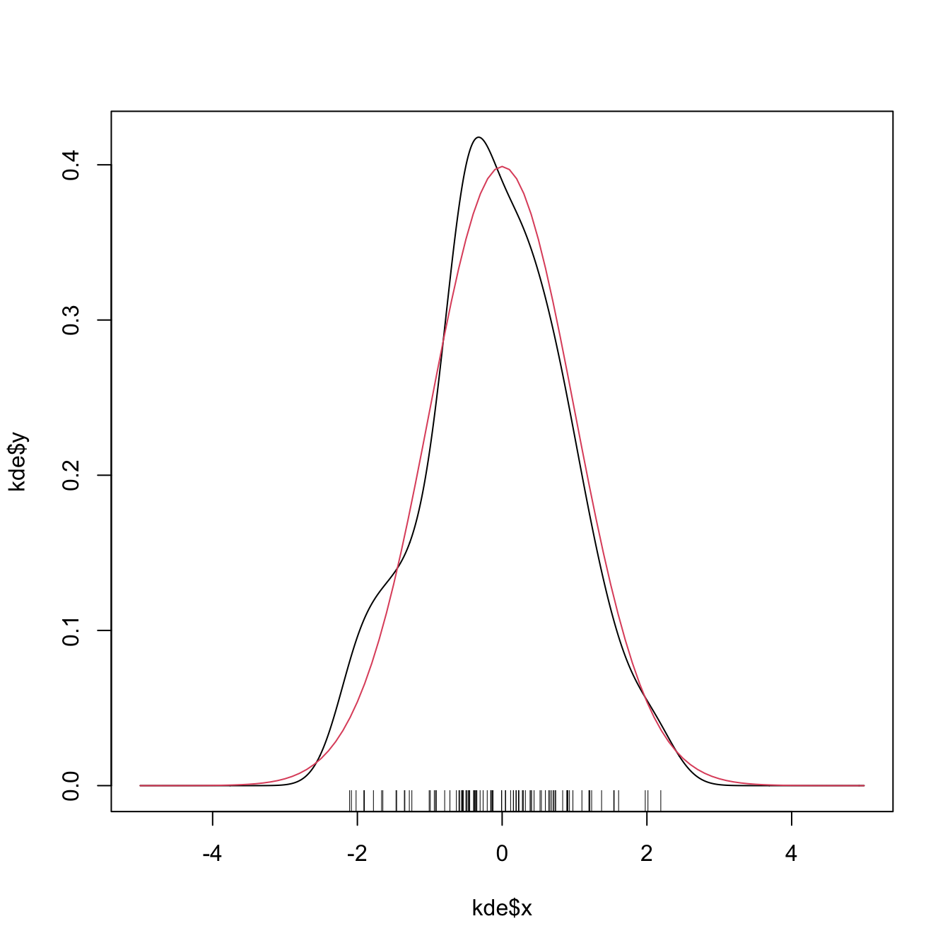

Exercise 6.1 Load the dataset faithful. Then:

Estimate and plot the density of faithful$eruptions.
Create a new plot and superimpose different density estimations with bandwidths equal to $0.1,$ $0.5,$ and $1.$
Get the density estimate at exactly the point $x=3.1$ using $h=0.15$ and the Epanechnikov kernel.

6.1.3 Bandwidth selection

The kde critically depends on the employed bandwidth; hence objective and automatic bandwidth selectors that attempt to minimize the estimation error of the target density $f$ are required to properly apply a kde in practice.

A global, rather than local, error criterion for the kde is the Integrated Squared Error (ISE):

\[\begin{align*} \mathrm{ISE}[\hat{f}(\cdot;h)]:=\int (\hat{f}(x;h)-f(x))^2\,\mathrm{d}x. \end{align*}\]

The ISE is a random quantity, since it depends directly on the sample $X_1,\ldots,X_n.$ As a consequence, looking for an optimal-ISE bandwidth is a hard task, since the optimality is dependent on the sample itself (not only on $f$ and $n$). To avoid this problem, it is usual to compute the Mean Integrated Squared Error (MISE):

\[\begin{align*} \mathrm{MISE}[\hat{f}(\cdot;h)]:=&\,\mathbb{E}\left[\mathrm{ISE}[\hat{f}(\cdot;h)]\right]\\ =&\,\int \mathbb{E}\left[(\hat{f}(x;h)-f(x))^2\right]\,\mathrm{d}x\\ =&\,\int \mathrm{MSE}[\hat{f}(x;h)]\,\mathrm{d}x. \end{align*}\]

Once the MISE is set as the error criterion to be minimized, our aim is to find

\[\begin{align*} h_\mathrm{MISE}:=\arg\min_{h>0}\mathrm{MISE}[\hat{f}(\cdot;h)]. \end{align*}\]

For that purpose, we need an explicit expression of the MISE that we can attempt to minimize. An asymptotic expansion can be derived when $h\to0$ and $nh\to\infty,$ resulting in

\[\begin{align} \mathrm{MISE}[\hat{f}(\cdot;h)]\approx\mathrm{AMISE}[\hat{f}(\cdot;h)]:=\frac{1}{4}\mu^2_2(K)R(f'')h^4+\frac{R(K)}{nh},\tag{6.5} \end{align}\]

where $\mu_2(K):=\int z^2K(z)\,\mathrm{d}z$ and $R(g):=\int g(x)^2\,\mathrm{d}x.$ The AMISE stands for Asymptotic MISE and, due to its closed expression, it allows to obtain a bandwidth that minimizes it:¹⁹⁷

\[\begin{align} h_\mathrm{AMISE}=\left[\frac{R(K)}{\mu_2^2(K)R(f'')n}\right]^{1/5}.\tag{6.6} \end{align}\]

Unfortunately, the AMISE bandwidth depends on $R(f'')=\int(f''(x))^2\,\mathrm{d}x,$ which measures the curvature of the unknown density $f.$ As a consequence, it cannot be readily applied in practice!

6.1.3.1 Plug-in selectors

A simple solution to turn (6.6) into something computable is to estimate $R(f'')$ by assuming that $f$ is the density of a $\mathcal{N}(\mu,\sigma^2),$ and then plug-in the form of the curvature for such density:

\[\begin{align*} R(\phi''(\cdot;\mu,\sigma^2))=\frac{3}{8\pi^{1/2}\sigma^5}. \end{align*}\]

While doing so, we approximate the curvature of an arbitrary density by means of the curvature of a normal and we have that

\[\begin{align*} h_\mathrm{AMISE}=\left[\frac{8\pi^{1/2}R(K)}{3\mu_2^2(K)n}\right]^{1/5}\sigma. \end{align*}\]

Interestingly, the bandwidth is directly proportional to the standard deviation of the target density. Replacing $\sigma$ by an estimate yields the normal scale bandwidth selector, which we denote by $\hat{h}_\mathrm{NS}$ to emphasize its randomness:

\[\begin{align*} \hat{h}_\mathrm{NS}=\left[\frac{8\pi^{1/2}R(K)}{3\mu_2^2(K)n}\right]^{1/5}\hat\sigma. \end{align*}\]

The estimate $\hat\sigma$ can be chosen as the standard deviation $s,$ or, in order to avoid the effects of potential outliers, as the standardized interquantile range

\[\begin{align*} \hat \sigma_{\mathrm{IQR}}:=\frac{X_{([0.75n])}-X_{([0.25n])}}{\Phi^{-1}(0.75)-\Phi^{-1}(0.25)} \end{align*}\]

or as

\[\begin{align} \hat\sigma=\min(s,\hat \sigma_{\mathrm{IQR}}). \tag{6.7} \end{align}\]

When combined with a normal kernel, for which $\mu_2(K)=1$ and $R(K)=\frac{1}{2\sqrt{\pi}},$ this particularization of $\hat{h}_{\mathrm{NS}}$ gives the famous rule-of-thumb for bandwidth selection:

\[\begin{align*} \hat{h}_\mathrm{RT}=\left(\frac{4}{3}\right)^{1/5}n^{-1/5}\hat\sigma\approx1.06n^{-1/5}\hat\sigma. \end{align*}\]

$\hat{h}_{\mathrm{RT}}$ is implemented in R through the function bw.nrd.¹⁹⁸

# Data
set.seed(667478)
n <- 100
x <- rnorm(n)

# Rule-of-thumb
bw.nrd(x = x)
## [1] 0.4040319
# bwd.nrd employs 1.34 as an approximation for diff(qnorm(c(0.25, 0.75)))

# Same as
iqr <- diff(quantile(x, c(0.25, 0.75))) / diff(qnorm(c(0.25, 0.75)))
1.06 * n^(-1/5) * min(sd(x), iqr)
## [1] 0.4040319

The rule-of-thumb is an example of a zero-stage plug-in selector, a terminology which rests on the fact that $R(f'')$ was estimated by plugging-in a parametric estimation at “the very first moment a quantity that depends on $f$ appears”. We could have opted to estimate $R(f'')$ nonparametrically, in a certain optimal way, and then plug-in the estimate into $h_\mathrm{AMISE}.$ The important catch lies on the optimal estimation of $R(f'')$ : it requires the knowledge of $R\big(f^{(4)}\big)$! What $\ell$-stage plug-in selectors do is to iterate these steps $\ell$ times and finally plug-in a normal estimate of the unknown $R\big(f^{(2\ell)}\big).$¹⁹⁹

Typically, two stages are considered a good trade-off between bias (mitigated when $\ell$ increases) and variance (increases with $\ell$) of the plug-in selector. This is the method proposed by Sheather and Jones (1991), yielding what we call the Direct Plug-In (DPI). The DPI selector is implemented in R through the function bw.SJ (use method = "dpi"). An alternative and faster implementation is ks::hpi, which also provides more flexibility and has a somewhat more detailed documentation.

# Data
set.seed(672641)
x <- rnorm(100)

# DPI selector
bw.SJ(x = x, method = "dpi")
## [1] 0.5006905

# Similar to
ks::hpi(x) # Default is two-stages
## [1] 0.4999456

6.1.3.2 Cross-validation

We turn now our attention to a different philosophy of bandwidth estimation. Instead of trying to minimize the AMISE by plugging-in estimates for the unknown curvature term, we directly attempt to minimize the MISE by using the sample twice: once for computing the kde and once for evaluating its performance on estimating $f.$ To avoid the clear dependence on the sample, we do the evaluation in a cross-validatory way: the data used for computing the kde is not used for its evaluation.

We begin by expanding the square in the MISE expression:

\[\begin{align*} \mathrm{MISE}[\hat{f}(\cdot;h)]=&\,\mathbb{E}\left[\int (\hat{f}(x;h)-f(x))^2\,\mathrm{d}x\right]\\ =&\,\mathbb{E}\left[\int \hat{f}(x;h)^2\,\mathrm{d}x\right]-2\mathbb{E}\left[\int \hat{f}(x;h)f(x)\,\mathrm{d}x\right]\\ &+\int f(x)^2\,\mathrm{d}x. \end{align*}\]

Since the last term does not depend on $h,$ minimizing $\mathrm{MISE}[\hat{f}(\cdot;h)]$ is equivalent to minimizing

\[\begin{align*} \mathbb{E}\left[\int \hat{f}(x;h)^2\,\mathrm{d}x\right]-2\mathbb{E}\left[\int \hat{f}(x;h)f(x)\,\mathrm{d}x\right]. \end{align*}\]

This quantity is unknown, but it can be estimated unbiasedly by

\[\begin{align} \mathrm{LSCV}(h):=\int\hat{f}(x;h)^2\,\mathrm{d}x-2n^{-1}\sum_{i=1}^n\hat{f}_{-i}(X_i;h),\tag{6.8} \end{align}\]

where $\hat{f}_{-i}(\cdot;h)$ is the leave-one-out kde and is based on the sample with the $X_i$ removed:

\[\begin{align*} \hat{f}_{-i}(x;h)=\frac{1}{n-1}\sum_{\substack{j=1\\j\neq i}}^n K_h(x-X_j). \end{align*}\]

The Least Squares Cross-Validation (LSCV) selector, also denoted Unbiased Cross-Validation (UCV) selector, is defined as

\[\begin{align*} \hat{h}_\mathrm{LSCV}:=\arg\min_{h>0}\mathrm{LSCV}(h). \end{align*}\]

Numerical optimization is required for obtaining $\hat{h}_\mathrm{LSCV},$ contrary to the previous plug-in selectors, and there is little control on the shape of the objective function.

Numerical optimization of the (6.8) can be challenging. In practice, several local minima are possible, and the roughness of the objective function can vary notably depending on $n$ and $f.$ As a consequence, optimization routines may get trapped in spurious solutions. To be on the safe side, it is advisable to check the solution by plotting $\mathrm{LSCV}(h)$ for a range of $h,$ or to perform an exhaustive search in a bandwidth grid: $\hat{h}_\mathrm{LSCV}\approx\arg\min_{h_1,\ldots,h_G}\mathrm{LSCV}(h).$

$\hat{h}_{\mathrm{LSCV}}$ is implemented in R through the function bw.ucv. bw.ucv uses optimize, which is quite sensitive to the selection of the search interval.²⁰⁰ Therefore, some care is needed and that is why the bw.ucv.mod function is presented.

# Data
set.seed(123456)
x <- rnorm(100)

# UCV gives a warning
bw.ucv(x = x)
## [1] 0.4499177

# Extend search interval
bw.ucv(x = x, lower = 0.01, upper = 1)
## [1] 0.5482419

# bw.ucv.mod replaces the optimization routine of bw.ucv by an exhaustive
# search on "h.grid" (chosen adaptatively from the sample) and optionally
# plots the LSCV curve with "plot.cv"
bw.ucv.mod <- function(x, nb = 1000L,
                       h.grid = diff(range(x)) * (seq(0.1, 1, l = 200))^2,
                       plot.cv = FALSE) {
  if ((n <- length(x)) < 2L)
    stop("need at least 2 data points")
  n <- as.integer(n)
  if (is.na(n))
    stop("invalid length(x)")
  if (!is.numeric(x))
    stop("invalid 'x'")
  nb <- as.integer(nb)
  if (is.na(nb) || nb <= 0L)
    stop("invalid 'nb'")
  storage.mode(x) <- "double"
  hmax <- 1.144 * sqrt(var(x)) * n^(-1/5)
  Z <- .Call(stats:::C_bw_den, nb, x)
  d <- Z[[1L]]
  cnt <- Z[[2L]]
  fucv <- function(h) .Call(stats:::C_bw_ucv, n, d, cnt, h)
  ## Original
  # h <- optimize(fucv, c(lower, upper), tol = tol)$minimum
  # if (h < lower + tol | h > upper - tol)
  #   warning("minimum occurred at one end of the range")
  ## Modification
  obj <- sapply(h.grid, function(h) fucv(h))
  h <- h.grid[which.min(obj)]
  if (plot.cv) {
    plot(h.grid, obj, type = "o")
    rug(h.grid)
    abline(v = h, col = 2, lwd = 2)
  }
  h
}

# Compute the bandwidth and plot the LSCV curve
bw.ucv.mod(x = x, plot.cv = TRUE)
## [1] 0.5431732

# We can compare with the default bw.ucv output
abline(v = bw.ucv(x = x), col = 3)

The next cross-validation selector is based on Biased Cross-Validation (BCV). The BCV selector presents a hybrid strategy that combines plug-in and cross-validation ideas. It starts by considering the AMISE expression in (6.5) and then plugs-in an estimate for $R(f'')$ based on a modification of $R(\hat{f}''(\cdot;h)).$ The appealing property of $\hat{h}_\mathrm{BCV}$ is that it has a considerably smaller variance compared to $\hat{h}_\mathrm{LSCV}.$ This reduction in variance comes at the price of an increased bias, which tends to make $\hat{h}_\mathrm{BCV}$ larger than $h_\mathrm{MISE}.$

$\hat{h}_{\mathrm{BCV}}$ is implemented in R through the function bw.bcv. Again, bw.bcv uses optimize so the bw.bcv.mod function is presented to have better guarantees on finding the adequate minimum.²⁰¹

# Data
set.seed(123456)
x <- rnorm(100)

# BCV gives a warning
bw.bcv(x = x)
## [1] 0.4500924

# Extend search interval
args(bw.bcv)
## function (x, nb = 1000L, lower = 0.1 * hmax, upper = hmax, tol = 0.1 * 
##     lower) 
## NULL
bw.bcv(x = x, lower = 0.01, upper = 1)
## [1] 0.5070129

# bw.bcv.mod replaces the optimization routine of bw.bcv by an exhaustive
# search on "h.grid" (chosen adaptatively from the sample) and optionally
# plots the BCV curve with "plot.cv"
bw.bcv.mod <- function(x, nb = 1000L,
                       h.grid = diff(range(x)) * (seq(0.1, 1, l = 200))^2,
                       plot.cv = FALSE) {
  if ((n <- length(x)) < 2L)
    stop("need at least 2 data points")
  n <- as.integer(n)
  if (is.na(n))
    stop("invalid length(x)")
  if (!is.numeric(x))
    stop("invalid 'x'")
  nb <- as.integer(nb)
  if (is.na(nb) || nb <= 0L)
    stop("invalid 'nb'")
  storage.mode(x) <- "double"
  hmax <- 1.144 * sqrt(var(x)) * n^(-1/5)
  Z <- .Call(stats:::C_bw_den, nb, x)
  d <- Z[[1L]]
  cnt <- Z[[2L]]
  fbcv <- function(h) .Call(stats:::C_bw_bcv, n, d, cnt, h)
  ## Original code
  # h <- optimize(fbcv, c(lower, upper), tol = tol)$minimum
  # if (h < lower + tol | h > upper - tol)
  #   warning("minimum occurred at one end of the range")
  ## Modification
  obj <- sapply(h.grid, function(h) fbcv(h))
  h <- h.grid[which.min(obj)]
  if (plot.cv) {
    plot(h.grid, obj, type = "o")
    rug(h.grid)
    abline(v = h, col = 2, lwd = 2)
  }
  h
}

# Compute the bandwidth and plot the BCV curve
bw.bcv.mod(x = x, plot.cv = TRUE)
## [1] 0.5130493

# We can compare with the default bw.bcv output
abline(v = bw.bcv(x = x), col = 3)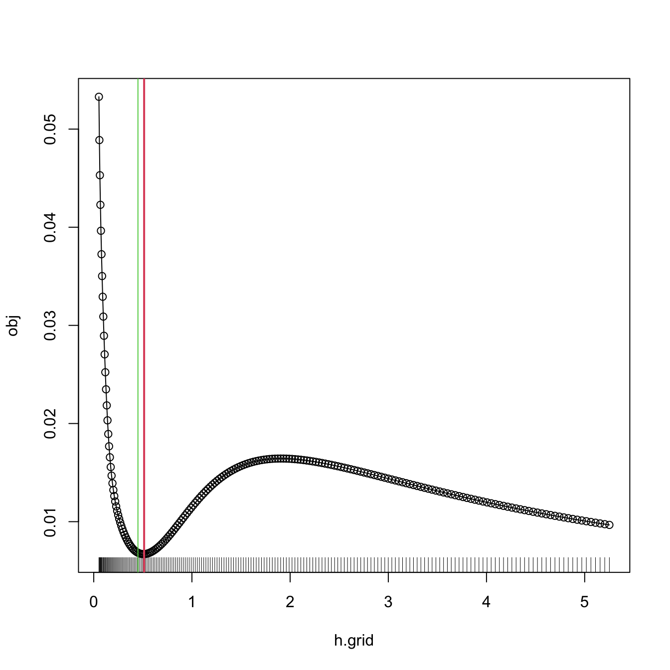

6.1.3.3 Comparison of bandwidth selectors

Although it is possible to compare theoretically the performance of bandwidth selectors by investigating the convergence of $n^\nu(\hat{h}/h_\mathrm{MISE}-1),$ comparisons are usually done by simulation and investigation of the averaged ISE error. A popular collection of simulation scenarios was given by Marron and Wand (1992) and are conveniently available through the package nor1mix. They form a collection of normal $r$-mixtures of the form

\[\begin{align*} f(x;\boldsymbol{\mu},\boldsymbol{\sigma},\mathbf{w}):&=\sum_{j=1}^rw_j\phi(x;\mu_j,\sigma_j^2), \end{align*}\]

where $w_j\geq0,$ $j=1,\ldots,r$ and $\sum_{j=1}^rw_j=1.$ Densities of this form are specially attractive since they allow for arbitrary flexibility and, if the normal kernel is employed, they allow for explicit and exact MISE expressions, directly computable as

\[\begin{align*} \mathrm{MISE}_r[\hat{f}(\cdot;h)]&=(2\sqrt{\pi}nh)^{-1}+\mathbf{w}^\top\{(1-n^{-1})\boldsymbol{\Omega}_2-2\boldsymbol{\Omega}_1+\boldsymbol{\Omega}_0\}\mathbf{w},\\ (\boldsymbol{\Omega}_a)_{ij}&:=\phi(\mu_i-\mu_j;ah^2+\sigma_i^2+\sigma_j^2),\quad i,j=1,\ldots,r. \end{align*}\]

This expression is especially useful for benchmarking bandwidth selectors, as the MISE optimal bandwidth can be computed by $h_\mathrm{MISE}=\arg\min_{h>0}\mathrm{MISE}_r[\hat{f}(\cdot;h)].$

# Available models
?nor1mix::MarronWand

# Simulating -- specify density with MW object
samp <- nor1mix::rnorMix(n = 500, obj = nor1mix::MW.nm9)
hist(samp, freq = FALSE)

# Density evaluation
x <- seq(-4, 4, length.out = 400)
lines(x, nor1mix::dnorMix(x = x, obj = nor1mix::MW.nm9), col = 2)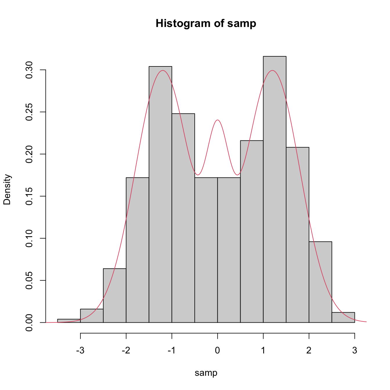


# Plot a MW object directly
# A normal with the same mean and variance is plotted in dashed lines
par(mfrow = c(2, 2))
plot(nor1mix::MW.nm5)
plot(nor1mix::MW.nm7)
plot(nor1mix::MW.nm10)
plot(nor1mix::MW.nm12)
lines(nor1mix::MW.nm1, col = 2:3) # Also possible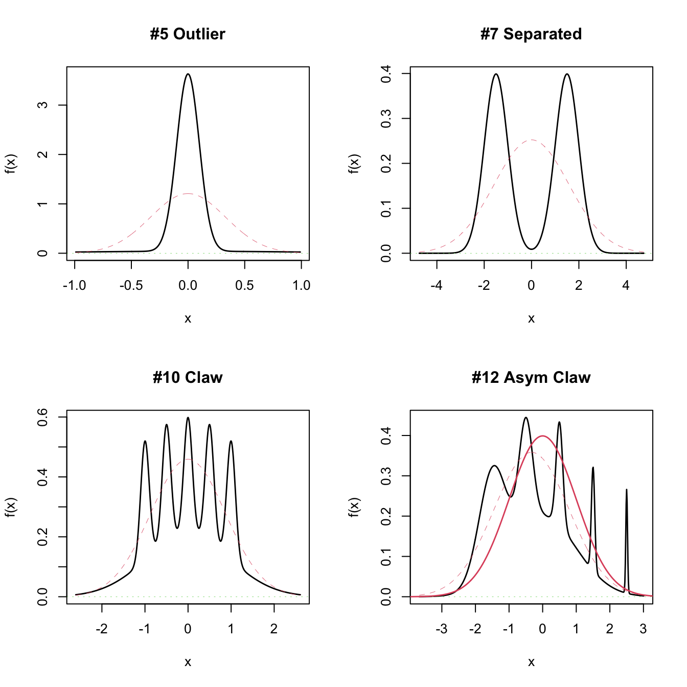

Figure 6.4 presents a visualization of the performance of the kde with different bandwidth selectors, carried out in the family of mixtures of Marron and Wand (1992).

Figure 6.4: Performance comparison of bandwidth selectors. The RT, DPI, LSCV, and BCV are computed for each sample for a normal mixture density. For each sample, computes the ISEs of the selectors and sorts them from best to worst. Changing the scenarios gives insight on the adequacy of each selector to hard- and simple-to-estimate densities. Application also available here.

Which bandwidth selector is the most adequate for a given dataset?

There is no simple and universal answer to this question. There are, however, a series of useful facts and suggestions:

Trying several selectors and inspecting the results may help on determining which one is estimating the density better.
The DPI selector has a convergence rate much faster than the cross-validation selectors. Therefore, in theory, it is expected to perform better than LSCV and BCV. For this reason, it tends to be amongst the preferred bandwidth selectors in the literature.
Cross-validatory selectors may be better suited for highly non-normal and rough densities, in which plug-in selectors may end up oversmoothing.
LSCV tends to be considerably more variable than BCV.
The RT is a quick, simple, and inexpensive selector. However, it tends to give bandwidths that are too large for non-normal data.

6.1.4 Multivariate extension

Kernel density estimation can be extended to estimate multivariate densities $f$ in $\mathbb{R}^p.$ For a sample $\mathbf{X}_1,\ldots,\mathbf{X}_n$ in $\mathbb{R}^p,$ the kde of $f$ evaluated at $\mathbf{x}\in\mathbb{R}^p$ is

\[\begin{align} \hat{f}(\mathbf{x};\mathbf{H}):=\frac{1}{n|\mathbf{H}|^{1/2}}\sum_{i=1}^nK\left(\mathbf{H}^{-1/2}(\mathbf{x}-\mathbf{X}_i)\right),\tag{6.9} \end{align}\]

where $K$ is multivariate kernel, a $p$-variate density that is (typically) symmetric and unimodal at $\mathbf{0},$ and that depends on the bandwidth matrix²⁰² $\mathbf{H},$ a $p\times p$ symmetric and positive definite matrix. A common notation is $K_\mathbf{H}(\mathbf{z}):=|\mathbf{H}|^{-1/2}K\big(\mathbf{H}^{-1/2}\mathbf{z}\big),$ so the kde can be compactly written as $\hat{f}(\mathbf{x};\mathbf{H}):=\frac{1}{n}\sum_{i=1}^nK_\mathbf{H}(\mathbf{x}-\mathbf{X}_i).$ The most employed multivariate kernel is the normal kernel $K(\mathbf{z})=\phi(\mathbf{z};\mathbf{0},\mathbf{I}_p).$

The interpretation of (6.9) is analogous to the one of (6.4): build a mixture of densities with each density centered at each data point. As a consequence, and roughly speaking, most of the concepts and ideas seen in univariate kernel density estimation extend to the multivariate situation, although some of them with considerable technical complications. For example, bandwidth selection inherits the same cross-validatory ideas (LSCV and BCV selectors) and plug-in methods (NS and DPI) seen before, but with increased complexity for the BCV and DPI selectors. The interested reader is referred to Chacón and Duong (2018) for a rigorous and comprehensive treatment.

We briefly discuss next the NS and LSCV selectors, denoted by $\hat{\mathbf{H}}_\mathrm{NS}$ and $\hat{\mathbf{H}}_\mathrm{LSCV},$ respectively. The normal scale bandwidth selector follows, as in the univariate case, by minimizing the asymptotic MISE of the kde, which now takes the form

\[\begin{align*} \mathrm{MISE}[\hat{f}(\cdot;\mathbf{H})]=\mathbb{E}\left[\int (\hat{f}(\mathbf{x};\mathbf{H})-f(\mathbf{x}))^2\,\mathrm{d}\mathbf{x}\right], \end{align*}\]

and then assuming that $f$ is the pdf of a $\mathcal{N}_p\left(\boldsymbol{\mu},\boldsymbol{\Sigma}\right).$ With the normal kernel, this results in

\[\begin{align} \mathbf{H}_\mathrm{NS}=(4(p+2))^{2/(p+4)}n^{-2/(p+4)}\boldsymbol{\Sigma}.\tag{6.10} \end{align}\]

Replacing $\boldsymbol{\Sigma}$ by the sample covariance matrix $\mathbf{S}$ in (6.10) gives $\hat{\mathbf{H}}_\mathrm{NS}.$

The unbiased cross-validation selector neatly extends from the univariate case and attempts to minimize $\mathrm{MISE}[\hat{f}(\cdot;\mathbf{H})]$ by estimating it unbiasedly with

\[\begin{align*} \mathrm{LSCV}(\mathbf{H}):=\int\hat{f}(\mathbf{x};\mathbf{H})^2\,\mathrm{d}\mathbf{x}-2n^{-1}\sum_{i=1}^n\hat{f}_{-i}(\mathbf{X}_i;\mathbf{H}) \end{align*}\]

and then minimizing it:

\[\begin{align} \hat{\mathbf{H}}_\mathrm{LSCV}:=\arg\min_{\mathbf{H}\in\mathrm{SPD}_p}\mathrm{LSCV}(\mathbf{H}),\tag{6.11} \end{align}\]

where $\mathrm{SPD}_p$ is the set of positive definite matrices²⁰³ of size $p.$

Considering a full bandwidth matrix $\mathbf{H}$ gives more flexibility to the kde, but also increases notably the amount of bandwidth parameters that need to be chosen – precisely $\frac{p(p+1)}{2}$ – which significantly complicates bandwidth selection as the dimension $p$ grows. A common simplification is to consider a diagonal bandwidth matrix $\mathbf{H}=\mathrm{diag}(h_1^2,\ldots,h_p^2),$ which yields the kde employing product kernels:

\[\begin{align} \hat{f}(\mathbf{x};\mathbf{h})=\frac{1}{n}\sum_{i=1}^nK_{h_1}(x_1-X_{i,1})\times\stackrel{p}{\cdots}\times K_{h_p}(x_p-X_{i,p}),\tag{6.12} \end{align}\]

where $\mathbf{h}=(h_1,\ldots,h_p)^\top$ is the vector of bandwidths. If the variables $X_1,\ldots,X_p$ have been standardized (so that they have the same scale), then a simple choice is to consider $h=h_1=\cdots=h_p.$

Multivariate kernel density estimation and bandwidth selection is not supported in base R, but the ks package implements the kde by ks::kde for $p\leq6.$ Bandwidth selectors, allowing for full or diagonal bandwidth matrices are implemented by: ks::Hns (NS), ks::Hpi and ks::Hpi.diag (DPI), ks::Hlscv and ks::Hlscv.diag (LSCV), and ks::Hbcv and ks::Hbcv.diag (BCV). The next chunk of code illustrates their usage with the faithful dataset.

# DPI selectors
Hpi1 <- ks::Hpi(x = faithful)
Hpi1
##            [,1]       [,2]
## [1,] 0.06326802  0.6041862
## [2,] 0.60418624 11.1917775

# Compute kde (if H is missing, ks::Hpi is called)
kdeHpi1 <- ks::kde(x = faithful, H = Hpi1)

# Different representations
plot(kdeHpi1, display = "slice", cont = c(25, 50, 75))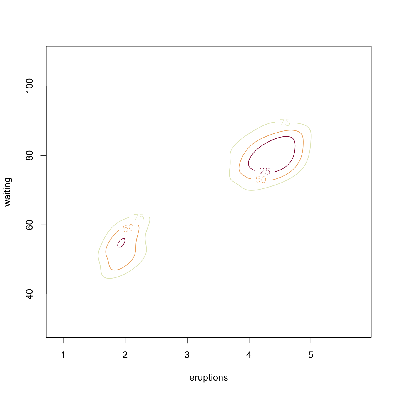

# "cont" specifies the density contours, which are upper percentages of highest
# density regions. The default contours are at 25%, 50%, and 75%
plot(kdeHpi1, display = "filled.contour2", cont = c(25, 50, 75))

plot(kdeHpi1, display = "persp")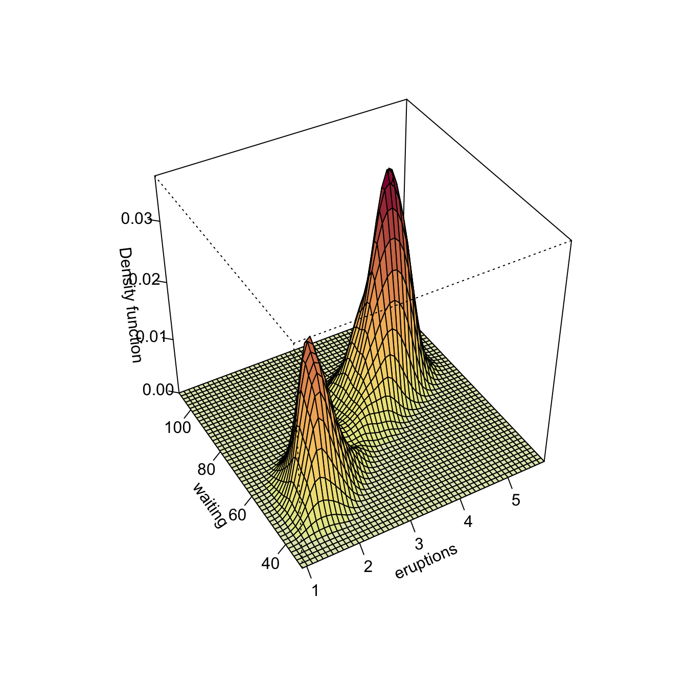


# Manual plotting using the kde object structure
image(kdeHpi1$eval.points[[1]], kdeHpi1$eval.points[[2]],
      kdeHpi1$estimate, col = viridis::viridis(20))
points(kdeHpi1$x)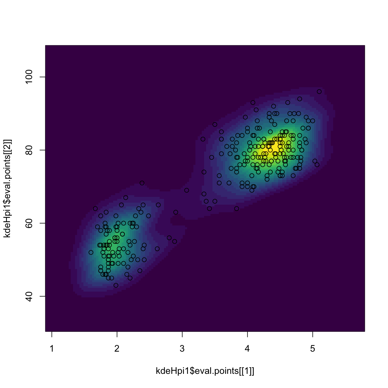


# Diagonal vs. full
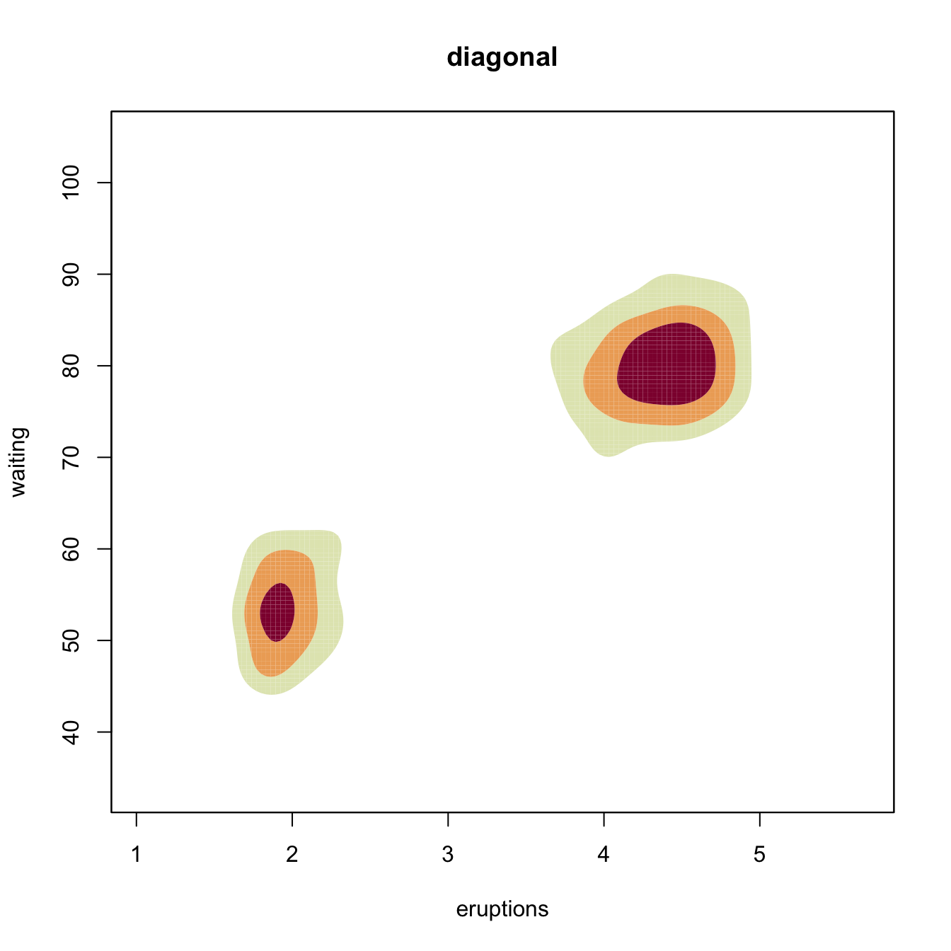
Hpi2 <- ks::Hpi.diag(x = faithful)
kdeHpi2 <- ks::kde(x = faithful, H = Hpi2)
plot(kdeHpi1, display = "filled.contour2", cont = c(25, 50, 75),
     main = "full")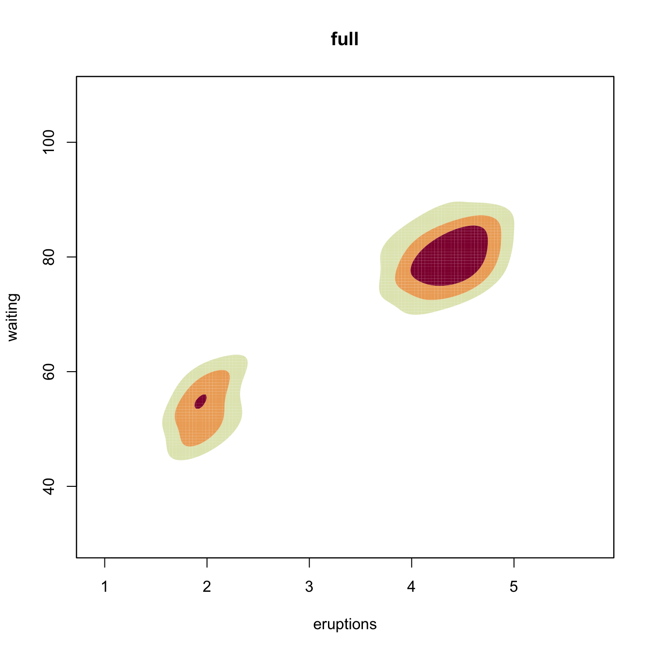

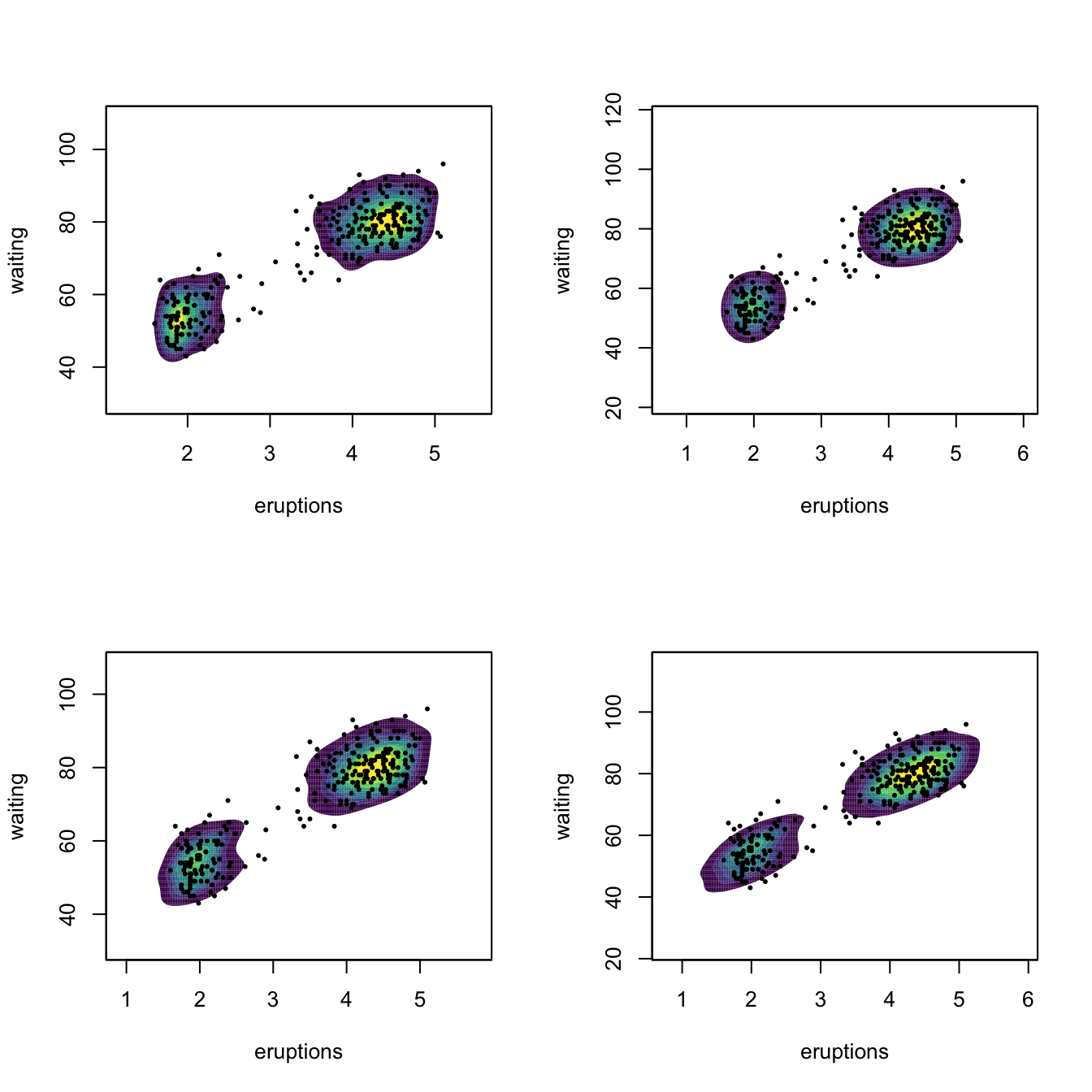
plot(kdeHpi2, display = "filled.contour2", cont = c(25, 50, 75),
     main = "diagonal")

# Comparison of selectors along predefined contours
x <- faithful
Hlscv0 <- ks::Hlscv(x = x)
Hbcv0 <- ks::Hbcv(x = x)
Hpi0 <- ks::Hpi(x = x)
Hns0 <- ks::Hns(x = x)
par(mfrow = c(2, 2))
p <- lapply(list(Hlscv0, Hbcv0, Hpi0, Hns0), function(H) {
  # col.fun for custom colors
  plot(ks::kde(x = x, H = H), display = "filled.contour2",
       cont = seq(10, 90, by = 10), col.fun = viridis::viridis)
  points(x, cex = 0.5, pch = 16)
})

Kernel density estimation can be used to visualize density level sets in 3D too, as illustrated as follows with the iris dataset.

# Normal scale bandwidth
Hns1 <- ks::Hns(iris[, 1:3])

# Show high nested contours of high density regions
plot(ks::kde(x = iris[, 1:3], H = Hns1))
rgl::points3d(x = iris[, 1:3])
rgl::rglwidget()

Exercise 6.2 Consider the normal mixture

\[\begin{align*} w_{1}\mathcal{N}_2(\mu_{11},\mu_{12},\sigma_{11}^2,\sigma_{12}^2,\rho_1)+w_{2}\mathcal{N}_2(\mu_{21},\mu_{22},\sigma_{21}^2,\sigma_{22}^2,\rho_2), \end{align*}\]

where $w_1=0.3,$ $w_2=0.7,$ $(\mu_{11}, \mu_{12})=(1, 1),$ $(\mu_{21}, \mu_{22})=(-1, -1),$ $\sigma_{11}^2=\sigma_{21}^2=1,$ $\sigma_{12}^2=\sigma_{22}^2=2,$ $\rho_1=0.5,$ and $\rho_2=-0.5.$

Perform the following simulation exercise:

Plot the density of the mixture using ks::dnorm.mixt and overlay points simulated employing ks::rnorm.mixt. You may want to use ks::contourLevels to have density plots comparable to the kde plots performed in the next step.
Compute the kde employing $\hat{\mathbf{H}}_{\mathrm{DPI}},$ both for full and diagonal bandwidth matrices. Are there any gains on considering full bandwidths? What if $\rho_2=0.7$?
Consider the previous point with $\hat{\mathbf{H}}_{\mathrm{LSCV}}$ instead of $\hat{\mathbf{H}}_{\mathrm{DPI}}.$ Are the conclusions the same?

6.2 Kernel regression estimation

6.2.1 Nadaraya–Watson estimator

Our objective is to estimate the regression function $m:\mathbb{R}^p\rightarrow\mathbb{R}$ nonparametrically (recall that we are considering the simplest situation: one continuous predictor, so $p=1$). Due to its definition, we can rewrite $m$ as

\[\begin{align} m(x)=&\,\mathbb{E}[Y \mid X=x]\nonumber\\ =&\,\int y f_{Y \mid X=x}(y)\,\mathrm{d}y\nonumber\\ =&\,\frac{\int y f(x,y)\,\mathrm{d}y}{f_X(x)}.\tag{6.13} \end{align}\]

This expression shows an interesting point: the regression function can be computed from the joint density $f$ and the marginal $f_X.$ Therefore, given a sample $\{(X_i,Y_i)\}_{i=1}^n,$ a nonparametric estimate of $m$ may follow by replacing the previous densities by their kernel density estimators! From the previous section, we know how to do this using the multivariate and univariate kde’s given in (6.4) and (6.9), respectively. For the multivariate kde, we can consider the kde (6.12) based on product kernels for the two dimensional case and bandwidths $\mathbf{h}=(h_1,h_2)^\top,$ which yields the estimate

\[\begin{align} \hat{f}(x,y;\mathbf{h})=\frac{1}{n}\sum_{i=1}^nK_{h_1}(x-X_{i})K_{h_2}(y-Y_{i})\tag{6.14} \end{align}\]

of the joint pdf of $(X,Y).$ On the other hand, considering the same bandwidth $h_1$ for the kde of $f_X,$ we have

\[\begin{align} \hat{f}_X(x;h_1)=\frac{1}{n}\sum_{i=1}^nK_{h_1}(x-X_{i}).\tag{6.15} \end{align}\]

We can therefore define the estimator of $m$ that results from replacing $f$ and $f_X$ in (6.13) by (6.14) and (6.15):

\[\begin{align*} \frac{\int y \hat{f}(x,y;\mathbf{h})\,\mathrm{d}y}{\hat{f}_X(x;h_1)}=&\,\frac{\int y \frac{1}{n}\sum_{i=1}^nK_{h_1}(x-X_i)K_{h_2}(y-Y_i)\,\mathrm{d}y}{\frac{1}{n}\sum_{i=1}^nK_{h_1}(x-X_i)}\\ =&\,\frac{\frac{1}{n}\sum_{i=1}^nK_{h_1}(x-X_i)\int y K_{h_2}(y-Y_i)\,\mathrm{d}y}{\frac{1}{n}\sum_{i=1}^nK_{h_1}(x-X_i)}\\ =&\,\frac{\frac{1}{n}\sum_{i=1}^nK_{h_1}(x-X_i)Y_i}{\frac{1}{n}\sum_{i=1}^nK_{h_1}(x-X_i)}\\ =&\,\sum_{i=1}^n\frac{K_{h_1}(x-X_i)}{\sum_{i=1}^nK_{h_1}(x-X_i)}Y_i. \end{align*}\]

The resulting estimator²⁰⁴ is the so-called Nadaraya–Watson²⁰⁵ estimator of the regression function:

\[\begin{align} \hat{m}(x;0,h):=\sum_{i=1}^n\frac{K_h(x-X_i)}{\sum_{i=1}^nK_h(x-X_i)}Y_i=\sum_{i=1}^nW^0_{i}(x)Y_i, \tag{6.16} \end{align}\]

where

\[\begin{align*} W^0_{i}(x):=\frac{K_h(x-X_i)}{\sum_{j=1}^nK_h(x-X_j)}. \end{align*}\]

The Nadaraya–Watson estimator can be seen as a weighted average of $Y_1,\ldots,Y_n$ by means of the set of weights $\{W_i(x)\}_{i=1}^n$ (they add to one). The set of varying weights depends on the evaluation point $x.$ That means that the Nadaraya–Watson estimator is a local mean of $Y_1,\ldots,Y_n$ about $X=x$ (see Figure 6.6).

Let’s implement from scratch the Nadaraya–Watson estimate to get a feeling of how it works in practice.

# A naive implementation of the Nadaraya-Watson estimator
mNW <- function(x, X, Y, h, K = dnorm) {

  # Arguments
  # x: evaluation points
  # X: vector (size n) with the predictors
  # Y: vector (size n) with the response variable
  # h: bandwidth
  # K: kernel

  # Matrix of size length(x) x n
  Kx <- sapply(X, function(Xi) K((x - Xi) / h) / h)

  # Weights
  W <- Kx / rowSums(Kx) # Column recycling!

  # Means at x ("drop" to drop the matrix attributes)
  drop(W %*% Y)

}

# Generate some data to test the implementation
set.seed(12345)
n <- 100
eps <- rnorm(n, sd = 2)
m <- function(x) x^2 * cos(x)
# m <- function(x) x - x^2 # Other possible regression function, works
# equally well
X <- rnorm(n, sd = 2)
Y <- m(X) + eps
xGrid <- seq(-10, 10, l = 500)

# Bandwidth
h <- 0.5

# Plot data
plot(X, Y)
rug(X, side = 1); rug(Y, side = 2)
lines(xGrid, m(xGrid), col = 1)
lines(xGrid, mNW(x = xGrid, X = X, Y = Y, h = h), col = 2)
legend("top", legend = c("True regression", "Nadaraya-Watson"),
       lwd = 2, col = 1:2)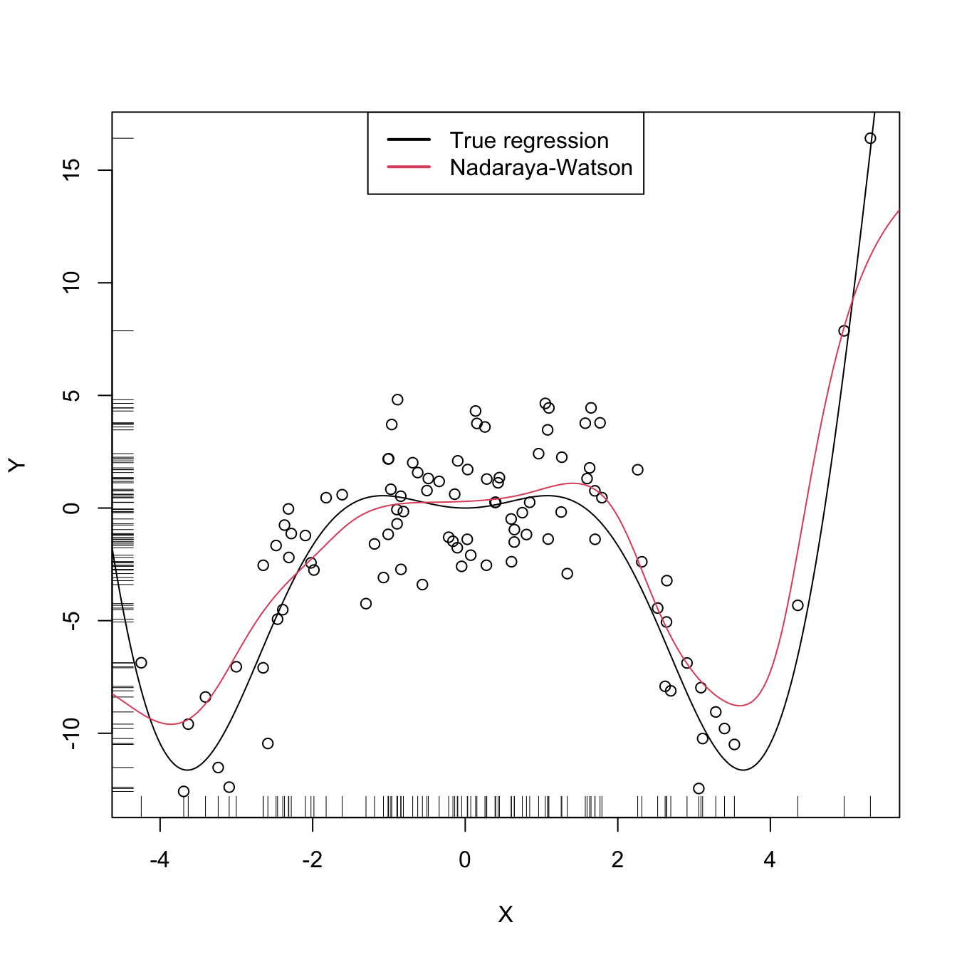

$The Nadaraya–Watson estimator of an arbitrary regression function $m$.$

Figure 6.5: The Nadaraya–Watson estimator of an arbitrary regression function $m$.

Similarly to kernel density estimation, in the Nadaraya–Watson estimator the bandwidth has a prominent effect on the shape of the estimator, whereas the kernel is clearly less important. The code below illustrates the effect of varying $h$ using the manipulate::manipulate function.

# Simple plot of N-W for varying h's
manipulate::manipulate({

  # Plot data
  plot(X, Y)
  rug(X, side = 1); rug(Y, side = 2)
  lines(xGrid, m(xGrid), col = 1)
  lines(xGrid, mNW(x = xGrid, X = X, Y = Y, h = h), col = 2)
  legend("topright", legend = c("True regression", "Nadaraya-Watson"),
         lwd = 2, col = 1:2)

}, h = manipulate::slider(min = 0.01, max = 2, initial = 0.5, step = 0.01))

Exercise 6.3 Implement your own version of the Nadaraya–Watson estimator in R and compare it with mNW. Focus only on the normal kernel and reduce the accuracy of the final computation up to 1e-7 to achieve better efficiency. Are you able to improve the speed of mNW? Use the microbenchmark::microbenchmark function to measure the running times for a sample with $n=10000.$

6.2.2 Local polynomial regression

The Nadaraya–Watson estimator can be seen as a particular case of a wider class of nonparametric estimators, the so called local polynomial estimators. Specifically, Nadaraya–Watson corresponds to performing a local constant fit. Let’s see this wider class of nonparametric estimators and their advantages with respect to the Nadaraya–Watson estimator.

The motivation for the local polynomial fit comes from attempting to find an estimator $\hat{m}$ of $m$ that “minimizes”²⁰⁶ the RSS

\[\begin{align} \sum_{i=1}^n(Y_i-\hat{m}(X_i))^2\tag{6.17} \end{align}\]

without assuming any particular form for the true $m.$ This is not achievable directly, since no knowledge on $m$ is available. Recall that what we did in parametric models was to assume a parametrization for $m.$ For example, in simple linear regression we assumed $m_{\boldsymbol{\beta}}(\mathbf{x})=\beta_0+\beta_1x,$ which allowed to tackle the minimization of (6.17) by means of solving

\[\begin{align*} m_{\hat{\boldsymbol{\beta}}}(\mathbf{x}):=\arg\min_{\boldsymbol{\beta}}\sum_{i=1}^n(Y_i-m_{\boldsymbol{\beta}}(X_i))^2. \end{align*}\]

The resulting $m_{\hat{\boldsymbol{\beta}}}$ is precisely the estimator that minimizes the RSS among all the linear estimators, that is, among the class of estimators that we have parametrized.

When $m$ has no available parametrization and can adopt any mathematical form, an alternative approach is required. The first step is to induce a local parametrization for $m.$ By a $p$-th²⁰⁷ order Taylor expression it is possible to obtain that, for $x$ close to $X_i,$

\[\begin{align} m(X_i)\approx&\, m(x)+m'(x)(X_i-x)+\frac{m''(x)}{2}(X_i-x)^2\nonumber\\ &+\cdots+\frac{m^{(p)}(x)}{p!}(X_i-x)^p.\tag{6.18} \end{align}\]

Then, replacing (6.18) in the population version of (6.17) that replaces $\hat{m}$ with $m,$ we have that

\[\begin{align} \sum_{i=1}^n\left(Y_i-\sum_{j=0}^p\frac{m^{(j)}(x)}{j!}(X_i-x)^j\right)^2.\tag{6.19} \end{align}\]

Expression (6.19) is still not workable: it depends on $m^{(j)}(x),$ $j=0,\ldots,p,$ which of course are unknown, as $m$ is unknown. The great idea is to set $\beta_j:=\frac{m^{(j)}(x)}{j!}$ and turn (6.19) into a linear regression problem where the unknown parameters are precisely $\boldsymbol{\beta}=(\beta_0,\beta_1,\ldots,\beta_p)^\top.$ Simply rewriting (6.19) using this idea gives

\[\begin{align} \sum_{i=1}^n\left(Y_i-\sum_{j=0}^p\beta_j(X_i-x)^j\right)^2.\tag{6.20} \end{align}\]

Now, estimates of $\boldsymbol{\beta}$ automatically produce estimates for $m^{(j)}(x)$! In addition, we know how to obtain an estimate $\hat{\boldsymbol{\beta}}$ that minimizes (6.20), since this is precisely the least squares problem studied in Section 2.2.3. The final touch is to weight the contributions of each datum $(X_i,Y_i)$ to the estimation of $m(x)$ according to the proximity of $X_i$ to $x.$²⁰⁸ We can achieve this precisely by kernels:

\[\begin{align} \hat{\boldsymbol{\beta}}_h:=\arg\min_{\boldsymbol{\beta}\in\mathbb{R}^{p+1}}\sum_{i=1}^n\left(Y_i-\sum_{j=0}^p\beta_j(X_i-x)^j\right)^2K_h(x-X_i).\tag{6.21} \end{align}\]

Solving (6.21) is easy once the proper notation is introduced. To that end, denote

\[\begin{align*} \mathbf{X}:=\begin{pmatrix} 1 & X_1-x & \cdots & (X_1-x)^p\\ \vdots & \vdots & \ddots & \vdots\\ 1 & X_n-x & \cdots & (X_n-x)^p\\ \end{pmatrix}_{n\times(p+1)} \end{align*}\]

and

\[\begin{align*} \mathbf{W}:=\mathrm{diag}(K_h(X_1-x),\ldots, K_h(X_n-x)),\quad \mathbf{Y}:=\begin{pmatrix} Y_1\\ \vdots\\ Y_n \end{pmatrix}_{n\times 1}. \end{align*}\]

Then we can re-express (6.21) into a weighted least squares problem²⁰⁹ whose exact solution is

\[\begin{align} \hat{\boldsymbol{\beta}}_h&=\arg\min_{\boldsymbol{\beta}\in\mathbb{R}^{p+1}} (\mathbf{Y}-\mathbf{X}\boldsymbol{\beta})^\top\mathbf{W}(\mathbf{Y}-\mathbf{X}\boldsymbol{\beta})\nonumber\\ &=(\mathbf{X}^\top\mathbf{W}\mathbf{X})^{-1}\mathbf{X}^\top\mathbf{W}\mathbf{Y}.\tag{6.22} \end{align}\]

The estimate²¹⁰ for $m(x)$ is therefore computed as

\[\begin{align} \hat{m}(x;p,h):=&\,\hat{\beta}_{h,0}\nonumber\\ =&\,\mathbf{e}_1^\top(\mathbf{X}^\top\mathbf{W}\mathbf{X})^{-1}\mathbf{X}^\top\mathbf{W}\mathbf{Y}\nonumber\\ =&\,\sum_{i=1}^nW^p_{i}(x)Y_i\tag{6.23} \end{align}\]

where

\[\begin{align*} W^p_{i}(x):=\mathbf{e}_1^\top(\mathbf{X}^\top\mathbf{W}\mathbf{X})^{-1}\mathbf{X}^\top\mathbf{W}\mathbf{e}_i \end{align*}\]

and $\mathbf{e}_i$ is the $i$-th canonical vector. Just as the Nadaraya–Watson was, the local polynomial estimator is a weighted linear combination of the responses.

Two cases deserve special attention on (6.23):

$p=0$ is the local constant estimator or the Nadaraya–Watson estimator. In this situation, the estimator has explicit weights, as we saw before:

\[\begin{align*} W_i^0(x)=\frac{K_h(x-X_i)}{\sum_{j=1}^nK_h(x-X_j)}. \end{align*}\]
$p=1$ is the local linear estimator, which has weights equal to:

\[\begin{align*} W_i^1(x)=\frac{1}{n}\frac{\hat{s}_2(x;h)-\hat{s}_1(x;h)(X_i-x)}{\hat{s}_2(x;h)\hat{s}_0(x;h)-\hat{s}_1(x;h)^2}K_h(x-X_i), \end{align*}\]

where $\hat{s}_r(x;h):=\frac{1}{n}\sum_{i=1}^n(X_i-x)^rK_h(x-X_i).$

Recall that the local polynomial fit is computationally more expensive than the local constant fit: $\hat{m}(x;p,h)$ is obtained as the solution of a weighted linear problem, whereas $\hat{m}(x;0,h)$ can be directly computed as a weighted mean of the responses.

Figure 6.6 illustrates the construction of the local polynomial estimator (up to cubic degree) and shows how $\hat\beta_0=\hat{m}(x;p,h),$ the intercept of the local fit, estimates $m$ at $x.$

Figure 6.6: Construction of the local polynomial estimator. The animation shows how local polynomial fits in a neighborhood of $x$ are combined to provide an estimate of the regression function, which depends on the polynomial degree, bandwidth, and kernel (gray density at the bottom). The data points are shaded according to their weights for the local fit at $x.$ Application available here.

The local polynomial estimator $\hat{m}(\cdot;p,h)$ of $m$ performs a series of weighted polynomial fits; as many as points $x$ on which $\hat{m}(\cdot;p,h)$ is to be evaluated.

An inefficient implementation of the local polynomial estimator can be done relatively straightforwardly from the previous insight and from expression (6.22). However, several R packages provide implementations, such as KernSmooth::locpoly and R’s loess²¹¹ (but this one has a different control of the bandwidth plus a set of other modifications). Below are some examples of their usage.

# Generate some data
set.seed(123456)
n <- 100
eps <- rnorm(n, sd = 2)
m <- function(x) x^3 * sin(x)
X <- rnorm(n, sd = 1.5)
Y <- m(X) + eps
xGrid <- seq(-10, 10, l = 500)

# KernSmooth::locpoly fits
h <- 0.25
lp0 <- KernSmooth::locpoly(x = X, y = Y, bandwidth = h, degree = 0,
                           range.x = c(-10, 10), gridsize = 500)
lp1 <- KernSmooth::locpoly(x = X, y = Y, bandwidth = h, degree = 1,
                           range.x = c(-10, 10), gridsize = 500)
# Provide the evaluation points by range.x and gridsize

# loess fits
span <- 0.25 # The default span is 0.75, which works very bad in this scenario
lo0 <- loess(Y ~ X, degree = 0, span = span)
lo1 <- loess(Y ~ X, degree = 1, span = span)
# loess employs an "span" argument that plays the role of an variable bandwidth
# "span" gives the proportion of points of the sample that are taken into
# account for performing the local fit about x and then uses a triweight kernel
# (not a normal kernel) for weighting the contributions. Therefore, the final
# estimate differs from the definition of local polynomial estimator, although
# the principles in which are based are the same

# Prediction at x = 2
x <- 2
lp1$y[which.min(abs(lp1$x - x))] # Prediction by KernSmooth::locpoly
## [1] 5.445975
predict(lo1, newdata = data.frame(X = x)) # Prediction by loess
##        1 
## 5.379652
m(x) # Reality
## [1] 7.274379

# Plot data
plot(X, Y)
rug(X, side = 1); rug(Y, side = 2)
lines(xGrid, m(xGrid), col = 1)
lines(lp0$x, lp0$y, col = 2)
lines(lp1$x, lp1$y, col = 3)
lines(xGrid, predict(lo0, newdata = data.frame(X = xGrid)), col = 2, lty = 2)
lines(xGrid, predict(lo1, newdata = data.frame(X = xGrid)), col = 3, lty = 2)
legend("bottom", legend = c("True regression", "Local constant (locpoly)",
                            "Local linear (locpoly)", "Local constant (loess)",
                            "Local linear (loess)"),
       lwd = 2, col = c(1:3, 2:3), lty = c(rep(1, 3), rep(2, 2)))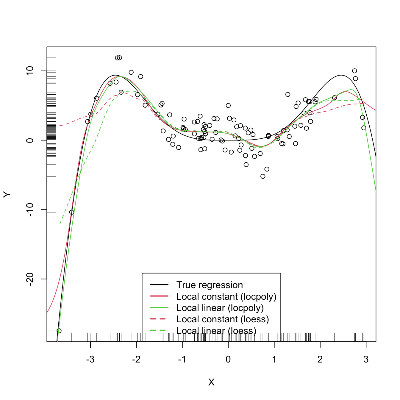

As with the Nadaraya–Watson, the local polynomial estimator heavily depends on $h.$

# Simple plot of local polynomials for varying h's
manipulate::manipulate({

  # Plot data
  lpp <- KernSmooth::locpoly(x = X, y = Y, bandwidth = h, degree = p,
                             range.x = c(-10, 10), gridsize = 500)
  plot(X, Y)
  rug(X, side = 1); rug(Y, side = 2)
  lines(xGrid, m(xGrid), col = 1)
  lines(lpp$x, lpp$y, col = p + 2)
  legend("bottom", legend = c("True regression", "Local polynomial fit"),
         lwd = 2, col = c(1, p + 2))

}, p = manipulate::slider(min = 0, max = 4, initial = 0, step = 1),
h = manipulate::slider(min = 0.01, max = 2, initial = 0.5, step = 0.01))

A more sophisticated framework for performing nonparametric estimation of the regression function is the np package, which we detail in Section 6.2.4. This package will be the chosen approach for the more challenging situation in which several predictors are present, since the former implementations do not scale well for more than one predictor.

6.2.3 Asymptotic properties

What affects the performance of the local polynomial estimator? Is local linear estimation better than local constant estimation? What is the effect of $h$?

The purpose of this section is to provide some highlights on the questions above by examining the theoretical properties of the local polynomial estimator. This is achieved by examining the asymptotic bias and variance of the local linear and local constant estimators.²¹² For this goal, we consider the location-scale model for $Y$ and its predictor $X$:

\[\begin{align*} Y=m(X)+\sigma(X)\varepsilon, \end{align*}\]

where $\sigma^2(x):=\mathbb{V}\mathrm{ar}[Y \mid X=x]$ is the conditional variance of $Y$ given $X$ and $\varepsilon$ is such that $\mathbb{E}[\varepsilon \mid X=x]]=0$ and $\mathbb{V}\mathrm{ar}[\varepsilon \mid X=x]]=1.$ Note that since the conditional variance is not forced to be constant we are implicitly allowing for heteroscedasticity.

The following assumptions²¹³ are the only requirements to perform the asymptotic analysis of the estimator:

A1.²¹⁴ $m$ is twice continuously differentiable.
A2.²¹⁵ $\sigma^2$ is continuous and positive.
A3.²¹⁶ $f,$ the marginal pdf of $X,$ is continuously differentiable and bounded away from zero.²¹⁷
A4.²¹⁸ The kernel $K$ is a symmetric and bounded pdf with finite second moment and is square integrable.
A5.²¹⁹ $h=h_n$ is a deterministic sequence of bandwidths such that, when $n\to\infty,$ $h\to0$ and $nh\to\infty.$

The bias and variance are studied in their conditional versions on the predictor’s sample $X_1,\ldots,X_n.$ The reason for analyzing the conditional instead of the unconditional versions is avoiding technical difficulties that integration with respect to the predictor’s density may pose. This is in the spirit of what it was done in the parametric inference of Sections 2.4 and 5.3. The main result is the following, which provides useful insights on the effect of $p,$ $m,$ $f$ (standing from now on for the marginal pdf of $X$), and $\sigma^2$ in the performance of $\hat{m}(\cdot;p,h).$

Theorem 6.1 Under A1–A5, the conditional bias and variance of the local constant ($p=0$) and local linear ($p=1$) estimators are²²⁰

\[\begin{align} \mathrm{Bias}[\hat{m}(x;p,h) \mid X_1,\ldots,X_n]&=B_p(x)h^2+o_\mathbb{P}(h^2),\tag{6.24}\\ \mathbb{V}\mathrm{ar}[\hat{m}(x;p,h) \mid X_1,\ldots,X_n]&=\frac{R(K)}{nhf(x)}\sigma^2(x)+o_\mathbb{P}((nh)^{-1}),\tag{6.25} \end{align}\]

where

\[\begin{align*} B_p(x):=\begin{cases} \frac{\mu_2(K)}{2}\left\{m''(x)+2\frac{m'(x)f'(x)}{f(x)}\right\},&\text{ if }p=0,\\ \frac{\mu_2(K)}{2}m''(x),&\text{ if }p=1. \end{cases} \end{align*}\]

The bias and variance expressions (6.24) and (6.25) yield very interesting insights:

Bias.
- The bias decreases with $h$ quadratically for both $p=0,1.$ That means that small bandwidths $h$ give estimators with low bias, whereas large bandwidths provide largely biased estimators.
- The bias at $x$ is directly proportional to $m''(x)$ if $p=1$ or affected by $m''(x)$ if $p=0.$ Therefore:
  - The bias is negative in regions where $m$ is concave, i.e., $\{x\in\mathbb{R}:m''(x)<0\}.$ These regions correspond to peaks and modes of $m$.
  - Conversely, the bias is positive in regions where $m$ is convex, i.e., $\{x\in\mathbb{R}:m''(x)>0\}.$ These regions correspond to valleys of $m$.
  - All in all, the “wilder” the curvature $m''$, the larger the bias and the harder to estimate $m$.
- The bias for $p=0$ at $x$ is affected by $m'(x),$ $f'(x),$ and $f(x).$ All of them are quantities that are not present in the bias when $p=1.$ Precisely, for the local constant estimator, the lower the density $f(x),$ the larger the bias. Also, the faster $m$ and $f$ change at $x$ (derivatives), the larger the bias. Thus the bias of the local constant estimator is much more sensible to $m(x)$ and $f(x)$ than the local linear (which is only sensible to $m''(x)$). Particularly, the fact that the bias depends on $f'(x)$ and $f(x)$ is referred to as the design bias since it depends merely on the predictor’s distribution.
Variance.
- The main term of the variance is the same for $p=0,1$. In addition, it depends directly on $\frac{\sigma^2(x)}{f(x)}.$ As a consequence, the lower the density, the more variable $\hat{m}(x;p,h)$ is.²²¹ Also, the larger the conditional variance at $x,$ $\sigma^2(x),$ the more variable $\hat{m}(x;p,h)$ is.²²²
- The variance decreases at a factor of $(nh)^{-1}$. This is related to the so-called effective sample size $nh,$ which can be thought of as the amount of data in the neighborhood of $x$ that is employed for performing the regression.²²³

The main takeaway of the analysis of $p=0$ vs. $p=1$ is that $p=1$ has smaller bias than $p=0$ (but of the same order) while keeping the same variance as $p=0$.

An extended version of Theorem 6.1, given in Theorem 3.1 of Fan and Gijbels (1996), shows that this phenomenon extends to higher orders: odd order ($p=2\nu+1,$ $\nu\in\mathbb{N}$) polynomial fits introduce an extra coefficient for the polynomial fit that allows them to reduce the bias, while maintaining the same variance of the precedent even order ($p=2\nu$). So, for example, local cubic fits are preferred to local quadratic fits. This motivates the claim that local polynomial fitting is an “odd world” (Fan and Gijbels (1996)).

6.2.4 Bandwidth selection

Bandwidth selection, as for density estimation, has a crucial practical importance for kernel regression estimation. Several bandwidth selectors have been proposed by following cross-validatory and plug-in ideas similar to the ones seen in Section 6.1.3. For simplicity, we briefly mention²²⁴ the DPI analogue for local linear regression for a single continuous predictor and focus mainly on least squares cross-validation, as it is a bandwidth selector that readily generalizes to the more complex settings of Section 6.3.

Following the derivation of the DPI for the kde, the first step is to define a suitable error criterion for the estimator $\hat{m}(\cdot;p,h).$ The conditional (on the sample of the predictor) MISE of $\hat{m}(\cdot;p,h)$ is often considered:

\[\begin{align*} \mathrm{MISE}[\hat{m}(\cdot;p,h) \mid X_1,\ldots,X_n]:=&\,\mathbb{E}\left[\int(\hat{m}(x;p,h)-m(x))^2f(x)\,\mathrm{d}x \mid X_1,\ldots,X_n\right]\\ =&\,\int\mathbb{E}\left[(\hat{m}(x;p,h)-m(x))^2 \mid X_1,\ldots,X_n\right]f(x)\,\mathrm{d}x\\ =&\,\int\mathrm{MSE}\left[\hat{m}(x;p,h) \mid X_1,\ldots,X_n\right]f(x)\,\mathrm{d}x. \end{align*}\]

Observe that this definition is very similar to the kde’s MISE, except for the fact that $f$ appears weighting the quadratic difference: what matters is to minimize the estimation error of $m$ on the regions where the density of $X$ is higher. Recall also that the MISE follows by integrating the conditional MSE, which amounts to the squared bias (6.24) plus the variance (6.25) given in Theorem 6.1. These operations produce the conditional AMISE:

\[\begin{align*} \mathrm{AMISE}[\hat{m}(\cdot;p,h) \mid X_1,\ldots,X_n]=&\,h^2\int B_p(x)^2f(x)\,\mathrm{d}x+\frac{R(K)}{nh}\int\sigma^2(x)\,\mathrm{d}x \end{align*}\]

and, if $p=1,$ the resulting optimal AMISE bandwidth is

\[\begin{align*} h_\mathrm{AMISE}=\left[\frac{R(K)\int\sigma^2(x)\,\mathrm{d}x}{2\mu_2^2(K)\theta_{22}n}\right]^{1/5}, \end{align*}\]

where $\theta_{22}:=\int(m''(x))^2f(x)\,\mathrm{d}x.$

As happened in the density setting, the AMISE-optimal bandwidth cannot be readily employed, as knowledge about the “curvature” of $m,$ $\theta_{22},$ and about $\int\sigma^2(x)\,\mathrm{d}x$ is required. As with the DPI selector, a series of nonparametric estimations of $\theta_{22}$ and high-order curvature terms follow, concluding with a necessary estimation of a higher-order curvature based on a “block polynomial fit”.²²⁵ The estimation of $\int\sigma^2(x)\,\mathrm{d}x$ is carried out by assuming homoscedasticity and a compactly supported density $f.$ The resulting bandwidth selector, $\hat{h}_\mathrm{DPI},$ has a much faster convergence rate to $h_{\mathrm{MISE}}$ than cross-validatory selectors. However, it is notably more convoluted, and as a consequence is less straightforward to extend to more complex settings.

The DPI selector for the local linear estimator is implemented in KernSmooth::dpill.

# Generate some data
set.seed(123456)
n <- 100
eps <- rnorm(n, sd = 2)
m <- function(x) x^3 * sin(x)
X <- rnorm(n, sd = 1.5)
Y <- m(X) + eps
xGrid <- seq(-10, 10, l = 500)

# DPI selector
hDPI <- KernSmooth::dpill(x = X, y = Y)

# Fits
lp1 <- KernSmooth::locpoly(x = X, y = Y, bandwidth = 0.25, degree = 0,
                           range.x = c(-10, 10), gridsize = 500)
lp1DPI <- KernSmooth::locpoly(x = X, y = Y, bandwidth = hDPI, degree = 1,
                              range.x = c(-10, 10), gridsize = 500)

# Compare fits
plot(X, Y)
rug(X, side = 1); rug(Y, side = 2)
lines(xGrid, m(xGrid), col = 1)
lines(lp1$x, lp1$y, col = 2)
lines(lp1DPI$x, lp1DPI$y, col = 3)
legend("bottom", legend = c("True regression", "Local linear",
                            "Local linear (DPI)"),
       lwd = 2, col = 1:3)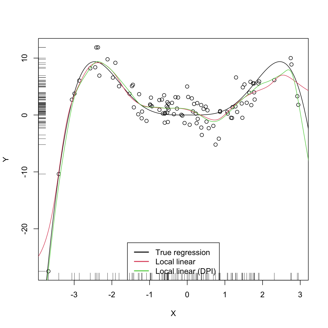

We turn now our attention to cross validation. Following an analogy with the fit of the linear model, we could look for the bandwidth $h$ such that it minimizes an RSS of the form

\[\begin{align} \frac{1}{n}\sum_{i=1}^n(Y_i-\hat{m}(X_i;p,h))^2.\tag{6.26} \end{align}\]

As it looks, this is a bad idea. Attempting to minimize (6.26) always leads to $h\approx 0$ that results in a useless interpolation of the data, as illustrated below.

# Grid for representing (6.26)
hGrid <- seq(0.1, 1, l = 200)^2
error <- sapply(hGrid, function(h) {
  mean((Y - mNW(x = X, X = X, Y = Y, h = h))^2)
})

# Error curve
plot(hGrid, error, type = "l")
rug(hGrid)
abline(v = hGrid[which.min(error)], col = 2)

As we know, the root of the problem is the comparison of $Y_i$ with $\hat{m}(X_i;p,h),$ since there is nothing forbidding $h\to0$ and as a consequence $\hat{m}(X_i;p,h)\to Y_i.$ As discussed in (3.17),²²⁶ a solution is to compare $Y_i$ with $\hat{m}_{-i}(X_i;p,h),$ the leave-one-out estimate of $m$ computed without the $i$-th datum $(X_i,Y_i),$ yielding the least squares cross-validation error

\[\begin{align} \mathrm{CV}(h)&:=\frac{1}{n}\sum_{i=1}^n(Y_i-\hat{m}_{-i}(X_i;p,h))^2\tag{6.27} \end{align}\]

and then choose

\[\begin{align*} \hat{h}_\mathrm{CV}&:=\arg\min_{h>0}\mathrm{CV}(h). \end{align*}\]

The optimization of (6.27) might seem as very computationally demanding, since it is required to compute $n$ regressions for just a single evaluation of the cross-validation function. There is, however, a simple and neat theoretical result that vastly reduces the computational complexity, at the price of increasing the memory demand. This trick allows us to compute, with a single fit, the cross-validation function.

Proposition 6.1 For any $p\geq0,$ the weights of the leave-one-out estimator $\hat{m}_{-i}(x;p,h)=\sum_{\substack{j=1\\j\neq i}}^nW_{-i,j}^p(x)Y_j$ can be obtained from $\hat{m}(x;p,h)=\sum_{i=1}^nW_{i}^p(x)Y_i$:

\[\begin{align*} W_{-i,j}^p(x)=\frac{W^p_j(x)}{\sum_{\substack{k=1\\k\neq i}}^nW_k^p(x)}=\frac{W^p_j(x)}{1-W_i^p(x)}. \end{align*}\]

This implies that

\[\begin{align} \mathrm{CV}(h)=\frac{1}{n}\sum_{i=1}^n\left(\frac{Y_i-\hat{m}(X_i;p,h)}{1-W_i^p(X_i)}\right)^2.\tag{6.28} \end{align}\]

The result can be proved using that the weights $\{W_{i}^p(x)\}_{i=1}^n$ add to one, for any $x,$ and that $\hat{m}(x;p,h)$ is a linear combination²²⁷ of the responses $\{Y_i\}_{i=1}^n.$

Computing (6.28) requires evaluating the local polynomial estimator at the sample $\{X_i\}_{i=1}^n$ and obtaining $\{W_i^p(X_i)\}_{i=1}^n$ (which are needed for evaluating $\hat{m}(X_i;p,h)$). Both tasks can be achieved simultaneously from the $n\times n$ matrix $\left(W_{i}^p(X_j)\right)_{ij}$ and, if $p=0,$ directly from the symmetric $n\times n$ matrix $\left(K_h(X_i-X_j)\right)_{ij},$ whose storage costs $\mathcal{O}\left(\frac{n^2-n}{2}\right)$ (the diagonal is constant).

Let’s implement $\hat{h}_\mathrm{CV}$ for the Nadaraya–Watson estimator.

# Generate some data to test the implementation
set.seed(12345)
n <- 100
eps <- rnorm(n, sd = 2)
m <- function(x) x^2 + sin(x)
X <- rnorm(n, sd = 1.5)
Y <- m(X) + eps
xGrid <- seq(-10, 10, l = 500)

# Objective function
cvNW <- function(X, Y, h, K = dnorm) {

  sum(((Y - mNW(x = X, X = X, Y = Y, h = h, K = K)) /
         (1 - K(0) / colSums(K(outer(X, X, "-") / h))))^2)
  # Beware: outer() is not very memory-friendly!

}

# Find optimum CV bandwidth, with sensible grid
bw.cv.grid <- function(X, Y,
                       h.grid = diff(range(X)) * (seq(0.1, 1, l = 200))^2,
                       K = dnorm, plot.cv = FALSE) {

    obj <- sapply(h.grid, function(h) cvNW(X = X, Y = Y, h = h, K = K))
  h <- h.grid[which.min(obj)]
  if (plot.cv) {
    plot(h.grid, obj, type = "o")
    rug(h.grid)
    abline(v = h, col = 2, lwd = 2)
  }
  h

}

# Bandwidth
hCV <- bw.cv.grid(X = X, Y = Y, plot.cv = TRUE)

hCV
## [1] 0.3117806

# Plot result
plot(X, Y)
rug(X, side = 1); rug(Y, side = 2)
lines(xGrid, m(xGrid), col = 1)
lines(xGrid, mNW(x = xGrid, X = X, Y = Y, h = hCV), col = 2)
legend("top", legend = c("True regression", "Nadaraya-Watson"),
       lwd = 2, col = 1:2)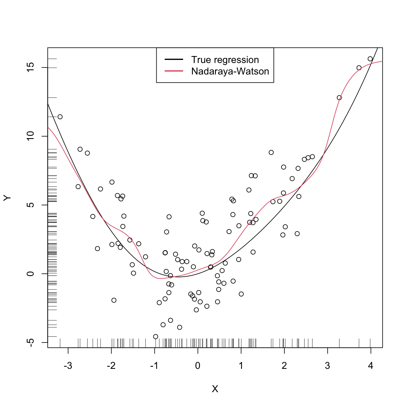

A more sophisticated cross-validation bandwidth selection can be achieved by np::npregbw and np::npreg, as shown in the code below.

# Turn off the "multistart" messages in the np package
options(np.messages = FALSE)

# np::npregbw computes by default the least squares CV bandwidth associated with
# a local constant fit
bw0 <- np::npregbw(formula = Y ~ X)

# Multiple initial points can be employed for minimizing the CV function (for
# one predictor, defaults to 1)
bw0 <- np::npregbw(formula = Y ~ X, nmulti = 2)

# The "rbandwidth" object contains many useful information, see ?np::npregbw for
# all the returned objects
bw0
## 
## Regression Data (100 observations, 1 variable(s)):
## 
##                       X
## Bandwidth(s): 0.3112962
## 
## Regression Type: Local-Constant
## Bandwidth Selection Method: Least Squares Cross-Validation
## Formula: Y ~ X
## Bandwidth Type: Fixed
## Objective Function Value: 5.368999 (achieved on multistart 1)
## 
## Continuous Kernel Type: Second-Order Gaussian
## No. Continuous Explanatory Vars.: 1
# Recall that the fit is very similar to hCV

# Once the bandwidth is estimated, np::npreg can be directly called with the
# "rbandwidth" object (it encodes the regression to be made, the data, the kind
# of estimator considered, etc). The hard work goes on np::npregbw, not on
# np::npreg
kre0 <- np::npreg(bw0)
kre0
## 
## Regression Data: 100 training points, in 1 variable(s)
##                       X
## Bandwidth(s): 0.3112962
## 
## Kernel Regression Estimator: Local-Constant
## Bandwidth Type: Fixed
## 
## Continuous Kernel Type: Second-Order Gaussian
## No. Continuous Explanatory Vars.: 1

# The evaluation points of the estimator are by default the predictor's sample
# (which is not sorted!)
# The evaluation of the estimator is given in "mean"
plot(kre0$eval$X, kre0$mean)


# The evaluation points can be changed using "exdat"
kre0 <- np::npreg(bw0, exdat = xGrid)

# Plot directly the fit via plot() -- it employs different evaluation points
# than exdat
plot(kre0, col = 2, type = "o")
points(X, Y)
rug(X, side = 1); rug(Y, side = 2)
lines(xGrid, m(xGrid), col = 1)
lines(kre0$eval$xGrid, kre0$mean, col = 3, type = "o", pch = 16, cex = 0.5)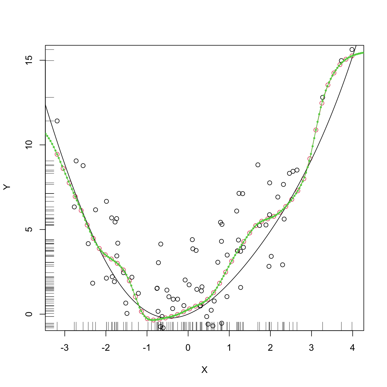

# Using the evaluation points

# Local linear fit -- find first the CV bandwidth
bw1 <- np::npregbw(formula = Y ~ X, regtype = "ll")
# regtype = "ll" stands for "local linear", "lc" for "local constant"

# Local linear fit
kre1 <- np::npreg(bw1, exdat = xGrid)

# Comparison
plot(X, Y)
rug(X, side = 1); rug(Y, side = 2)
lines(xGrid, m(xGrid), col = 1)
lines(kre0$eval$xGrid, kre0$mean, col = 2)
lines(kre1$eval$xGrid, kre1$mean, col = 3)
legend("top", legend = c("True regression", "Nadaraya-Watson", "Local linear"),
       lwd = 2, col = 1:3)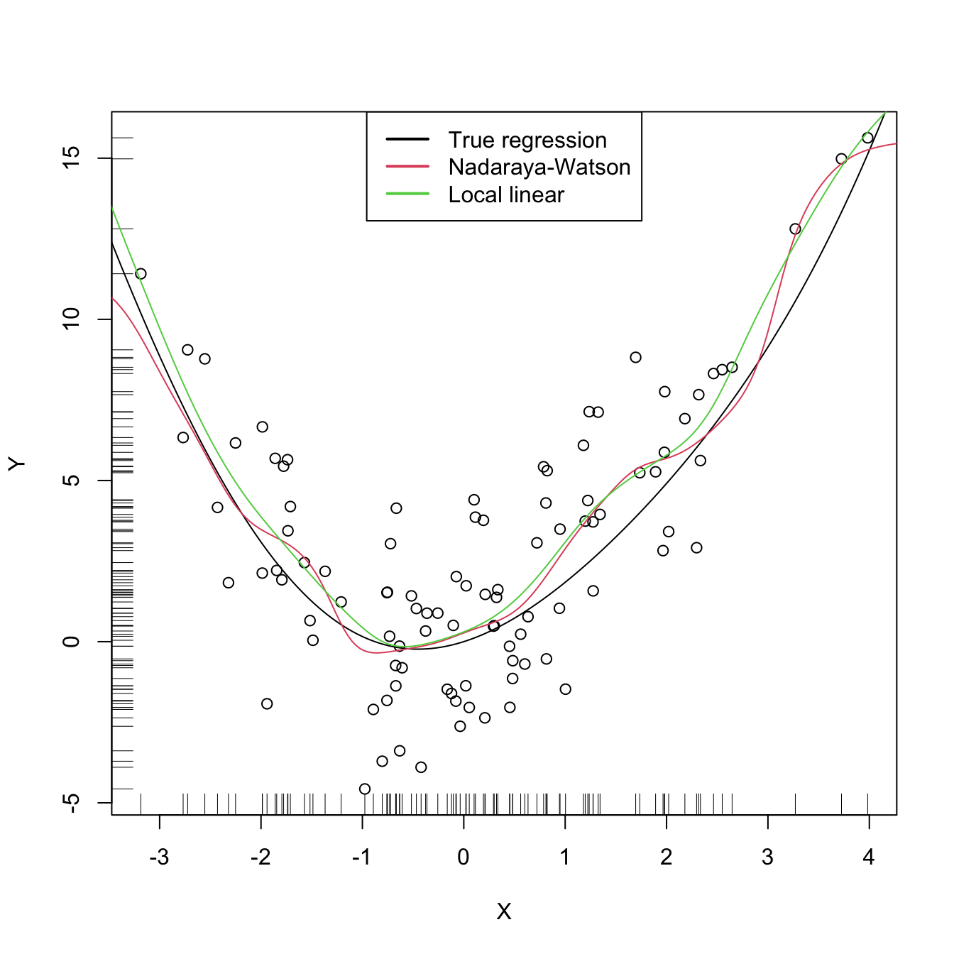

The adequate bandwidths for the local linear estimator are usually larger than the adequate bandwidths for the local constant estimator. The reason: the extra flexibility of the local linear estimator allows to adapt faster to variations in $m,$ whereas the local constant estimator can only achieve this by shrinking the neighborhood about $x$ by means of a small $h.$

There are more sophisticated options for bandwidth selection in np::npregbw. For example, the argument bwtype allows to estimate data-driven variable bandwidths $\hat{h}(x)$ that depend on the evaluation point $x,$ rather than fixed bandwidths $\hat{h},$ as we have considered. Roughly speaking, these variable bandwidths are related to the variable bandwidth $\hat{h}_k(x)$ that is necessary to contain the $k$ nearest neighbors $X_1,\ldots,X_k$ of $x$ in the neighborhood $(x-\hat{h}_k(x),x+\hat{h}_k(x)).$ There is a potential gain in employing variable bandwidths, as the estimator can adapt the amount of smoothing according to the density of the predictor. We do not investigate this approach in detail but just point to its implementation.

# Generate some data with bimodal density
set.seed(12345)
n <- 100
eps <- rnorm(2 * n, sd = 2)
m <- function(x) x^2 * sin(x)
X <- c(rnorm(n, mean = -2, sd = 0.5), rnorm(n, mean = 2, sd = 0.5))
Y <- m(X) + eps
xGrid <- seq(-10, 10, l = 500)

# Constant bandwidth
bwc <- np::npregbw(formula = Y ~ X, bwtype = "fixed", regtype = "ll")
krec <- np::npreg(bwc, exdat = xGrid)

# Variable bandwidths
bwg <- np::npregbw(formula = Y ~ X, bwtype = "generalized_nn", regtype = "ll")
kreg <- np::npreg(bwg, exdat = xGrid)
bwa <- np::npregbw(formula = Y ~ X, bwtype = "adaptive_nn", regtype = "ll")
krea <- np::npreg(bwa, exdat = xGrid)

# Comparison
plot(X, Y)
rug(X, side = 1); rug(Y, side = 2)
lines(xGrid, m(xGrid), col = 1)
lines(krec$eval$xGrid, krec$mean, col = 2)
lines(kreg$eval$xGrid, kreg$mean, col = 3)
lines(krea$eval$xGrid, krea$mean, col = 4)
legend("top", legend = c("True regression", "Fixed", "Generalized NN",
                         "Adaptive NN"),
       lwd = 2, col = 1:4)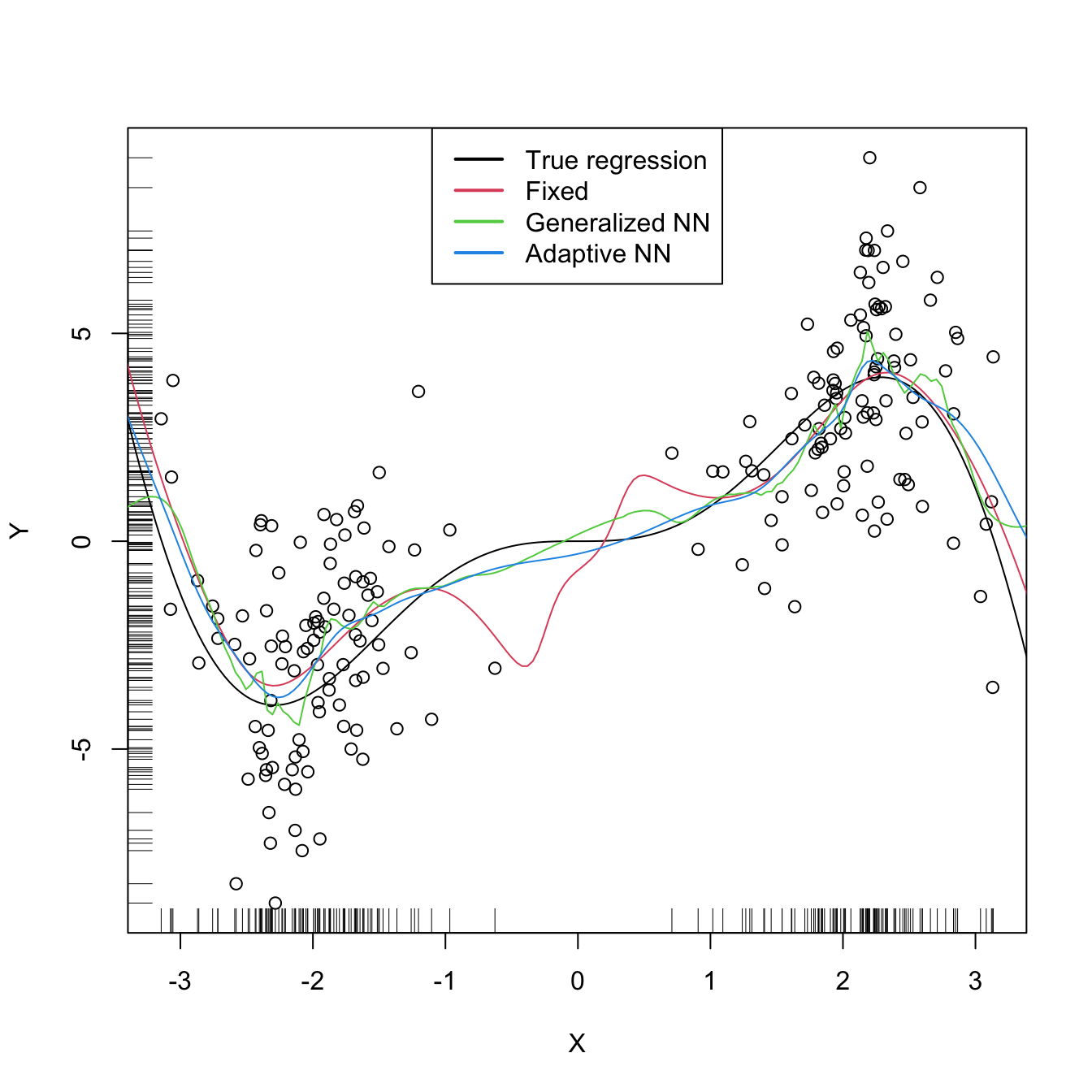

# Observe how the fixed bandwidth may yield a fit that produces serious
# artifacts in the low density region. At that region the NN-based bandwidths
# enlarge to borrow strength from the points in the high density regions,
# whereas in the high density regions they shrink to adapt faster to the
# changes of the regression function

6.3 Kernel regression with mixed multivariate data

Until now, we have studied the simplest situation for performing nonparametric estimation of the regression function: a single, continuous, predictor $X$ is available for explaining $Y,$ a continuous response. This served for introducing the main concepts without the additional technicalities associated with more complex predictors. We now extend the study to the case in which there are

multiple predictors $X_1,\ldots,X_p$ and
possible non-continuous predictors, namely categorical predictors and discrete predictors.

The first point is how to extend the local polynomial estimator $\hat{m}(\cdot;q,h)\;$²²⁸ to deal with $p$ continuous predictors. Although this can be done for $q\geq0,$ we focus on the local constant and linear estimators ($q=0,1$) for avoiding excessive technical complications.²²⁹ Also, to avoid a quick escalation of the number of smoothing bandwidths, it is customary to consider product kernels. With these two restrictions, the estimators for $m$ based on a sample $\{(\mathbf{X}_i,Y_i)\}_{i=1}^n$ extend easily from the developments in Sections 6.2.1 and 6.2.2:

Local constant estimator. We can replicate the argument in (6.13) with a multivariate kde for $f_{\mathbf{X}}$ based on product kernels with bandwidth vector $\mathbf{h},$ which gives

\[\begin{align*} \hat{m}(\mathbf{x};0,\mathbf{h}):=\sum_{i=1}^n\frac{K_\mathbf{h}(\mathbf{x}-\mathbf{X}_i)}{\sum_{i=1}^nK_\mathbf{h}(\mathbf{x}-\mathbf{X}_i)}Y_i=\sum_{i=1}^nW^0_{i}(\mathbf{x})Y_i \end{align*}\]

where

\[\begin{align*} K_\mathbf{h}(\mathbf{x}-\mathbf{X}_i)&:=K_{h_1}(x_1-X_{i1})\times\stackrel{p}{\cdots}\times K_{h_p}(x_p-X_{ip}),\\ W^0_{i}(\mathbf{x})&:=\frac{K_\mathbf{h}(\mathbf{x}-\mathbf{X}_i)}{\sum_{i=1}^nK_\mathbf{h}(\mathbf{x}-\mathbf{X}_i)}. \end{align*}\]
Local linear estimator. Considering the Taylor expansion $m(\mathbf{X}_i)\approx m(\mathbf{x})+\nabla m(\mathbf{x})(\mathbf{X}_i-\mathbf{x})\;$²³⁰ instead of (6.18) it is possible to arrive to the analogous of (6.21),

\[\begin{align*} \hat{\boldsymbol{\beta}}_\mathbf{h}:=\arg\min_{\boldsymbol{\beta}\in\mathbb{R}^{p+1}}\sum_{i=1}^n\left(Y_i-\boldsymbol{\beta}^\top(1,(\mathbf{X}_i-\mathbf{x})^\top)^\top\right)^2K_\mathbf{h}(\mathbf{x}-\mathbf{X}_i), \end{align*}\]

and then solve the problem in the exact same way but now considering

\[\begin{align*} \mathbf{X}:=\begin{pmatrix} 1 & (\mathbf{X}_1-\mathbf{x})^\top\\ \vdots & \vdots\\ 1 & (\mathbf{X}_n-\mathbf{x})^\top\\ \end{pmatrix}_{n\times(p+1)} \end{align*}\]

and

\[\begin{align*} \mathbf{W}:=\mathrm{diag}(K_{\mathbf{h}}(\mathbf{X}_1-\mathbf{x}),\ldots, K_\mathbf{h}(\mathbf{X}_n-\mathbf{x})). \end{align*}\]

The estimate²³¹ for $m(x)$ is therefore computed as

\[\begin{align*} \hat{m}(\mathbf{x};1,h):=&\,\hat{\beta}_{\mathbf{h},0}\\ =&\,\mathbf{e}_1^\top(\mathbf{X}^\top\mathbf{W}\mathbf{X})^{-1}\mathbf{X}^\top\mathbf{W}\mathbf{Y}\\ =&\,\sum_{i=1}^nW^1_{i}(\mathbf{x})Y_i \end{align*}\]

where

\[\begin{align*} W^1_{i}(\mathbf{x}):=\mathbf{e}_1^\top(\mathbf{X}^\top\mathbf{W}\mathbf{X})^{-1}\mathbf{X}^\top\mathbf{W}\mathbf{e}_i. \end{align*}\]

The cross-validation bandwidth selection rule studied on Section 6.2.4 extends neatly to the multivariate case:

\[\begin{align*} \mathrm{CV}(\mathbf{h})&:=\frac{1}{n}\sum_{i=1}^n(Y_i-\hat{m}_{-i}(\mathbf{X}_i;p,\mathbf{h}))^2,\\ \hat{\mathbf{h}}_\mathrm{CV}&:=\arg\min_{h_1,\ldots,h_p>0}\mathrm{CV}(\mathbf{h}). \end{align*}\]

Obvious complications appear in the optimization of $\mathrm{CV}(\mathbf{h}),$ which now is a $\mathbb{R}^p\rightarrow\mathbb{R}$ function. Importantly, the trick described in Proposition 6.1 also holds with obvious modifications.

Let’s see an application of multivariate kernel regression for the wine dataset.

# Employing the wine dataset
wine <- read.table(file = "wine.csv", header = TRUE, sep = ",")

# Bandwidth by CV for local linear estimator -- a product kernel with 4
# bandwidths. Employs 4 random starts for minimizing the CV surface
bwWine <- np::npregbw(formula = Price ~ Age + WinterRain + AGST + HarvestRain,
                      data = wine, regtype = "ll")
bwWine
## 
## Regression Data (27 observations, 4 variable(s)):
## 
##                   Age WinterRain      AGST HarvestRain
## Bandwidth(s): 3616691  290170218 0.8725243    106.5079
## 
## Regression Type: Local-Linear
## Bandwidth Selection Method: Least Squares Cross-Validation
## Formula: Price ~ Age + WinterRain + AGST + HarvestRain
## Bandwidth Type: Fixed
## Objective Function Value: 0.0873955 (achieved on multistart 4)
## 
## Continuous Kernel Type: Second-Order Gaussian
## No. Continuous Explanatory Vars.: 4

# Regression
fitWine <- np::npreg(bwWine)
summary(fitWine)
## 
## Regression Data: 27 training points, in 4 variable(s)
##                   Age WinterRain      AGST HarvestRain
## Bandwidth(s): 3616691  290170218 0.8725243    106.5079
## 
## Kernel Regression Estimator: Local-Linear
## Bandwidth Type: Fixed
## Residual standard error: 0.2079691
## R-squared: 0.8889649
## 
## Continuous Kernel Type: Second-Order Gaussian
## No. Continuous Explanatory Vars.: 4

# Plot marginal effects of each predictor on the response (the rest of
# predictors are fixed to their marginal medians)
plot(fitWine)
# Therefore:
# - Age is positively related to Price (almost linearly)
# - WinterRain is positively related to Price (with a subtle nonlinearity)
# - AGST is positively related to Price, but now we see what it looks like a
#   quadratic pattern
# - HarvestRain is negatively related to Price (almost linearly)

The $R^2$ outputted by the summary of np::npreg is defined as

\[\begin{align*} R^2:=\frac{(\sum_{i=1}^n(Y_i-\bar{Y})(\hat{Y}_i-\bar{Y}))^2}{(\sum_{i=1}^n(Y_i-\bar{Y})^2)(\sum_{i=1}^n(\hat{Y}_i-\bar{Y})^2)} \end{align*}\]

and is neither the $r^2_{y\hat{y}}$ (because it is not guaranteed that $\bar{Y}=\bar{\hat{Y}}$!) nor “the percentage of variance explained” by the model – this interpretation only makes sense within the linear model context. It is however a quantity in $[0,1]$ that attains $R^2=1$ when the fit is perfect.

Non-continuous variables can be taken into account by defining suitably adapted kernels. The two main possibilities for non-continuous data are:

Categorical or unordered discrete variables. For example, iris$species is a categorical variable in which ordering does not make sense. These variables are specified in R by factor. Due to the lack of ordering, the basic mathematical operation behind a kernel, a distance computation,²³² is senseless. That motivates the Aitchison and Aitken (1976) kernel.

Assume that the categorical random variable $X_d$ has $c_d$ different levels. Then, it can be represented as $X_d\in C_d:=\{0,1,\ldots,c_d-1\}.$ For $x_d,X_d\in C_d,$ the Aitchison and Aitken (1976) unordered discrete kernel is

\[\begin{align*} l(x_d,X_d;\lambda)=\begin{cases} 1-\lambda,&\text{ if }x_d=X_d,\\ \frac{\lambda}{c_d-1},&\text{ if }x_d\neq X_d, \end{cases} \end{align*}\]

where $\lambda\in[0,(c_d-1)/c_d]$ is the bandwidth.
Ordinal or ordered discrete variables. For example, wine$Year is a discrete variable with a clear order, but it is not continuous. These variables are specified by ordered (an ordered factor). In these variables there is ordering, but distances are discrete.

If the ordered discrete random variable $X_d$ can take $c_d$ different ordered values, then it can be represented as $X_d\in C_d:=\{0,1,\ldots,c_d-1\}.$ For $x_d,X_d\in C_d,$ a possible (Li and Racine 2007) ordered discrete kernel is

\[\begin{align*} l(x_d,X_d;\lambda)=\lambda^{|x_d-X_d|}, \end{align*}\]

where $\lambda\in[0,1]$ is the bandwidth.

The np package employs a variation of the previous kernels. The following examples illustrate their use.

# Bandwidth by CV for local linear estimator
# Recall that Species is a factor!
bwIris <- np::npregbw(formula = Petal.Length ~ Sepal.Width + Species,
                      data = iris, regtype = "ll")
bwIris
## 
## Regression Data (150 observations, 2 variable(s)):
## 
##               Sepal.Width      Species
## Bandwidth(s):    898696.6 2.357536e-07
## 
## Regression Type: Local-Linear
## Bandwidth Selection Method: Least Squares Cross-Validation
## Formula: Petal.Length ~ Sepal.Width + Species
## Bandwidth Type: Fixed
## Objective Function Value: 0.1541057 (achieved on multistart 1)
## 
## Continuous Kernel Type: Second-Order Gaussian
## No. Continuous Explanatory Vars.: 1
## 
## Unordered Categorical Kernel Type: Aitchison and Aitken
## No. Unordered Categorical Explanatory Vars.: 1
# Product kernel with 2 bandwidths

# Regression
fitIris <- np::npreg(bwIris)
summary(fitIris)
## 
## Regression Data: 150 training points, in 2 variable(s)
##               Sepal.Width      Species
## Bandwidth(s):    898696.6 2.357536e-07
## 
## Kernel Regression Estimator: Local-Linear
## Bandwidth Type: Fixed
## Residual standard error: 0.3775005
## R-squared: 0.9539633
## 
## Continuous Kernel Type: Second-Order Gaussian
## No. Continuous Explanatory Vars.: 1
## 
## Unordered Categorical Kernel Type: Aitchison and Aitken
## No. Unordered Categorical Explanatory Vars.: 1

# Plot marginal effects of each predictor on the response
par(mfrow = c(1, 2))
plot(fitIris, plot.par.mfrow = FALSE)

# Options for the plot method for np::npreg available at ?np::npplot
# For example, xq = 0.5 (default) indicates that all the predictors are set to
# their medians for computing the marginal effects

# Example from ?np::npreg: modeling of the GDP growth of a country from
# economic indicators of the country
# The predictors contain a mix of unordered, ordered, and continuous variables

# Load data
data(oecdpanel, package = "np")

# Bandwidth by CV for local constant -- use only two starts to reduce the
# computation time
bwOECD <- np::npregbw(formula = growth ~ factor(oecd) + ordered(year) +
                        initgdp + popgro + inv + humancap, data = oecdpanel,
                      regtype = "lc", nmulti = 2)
bwOECD
## 
## Regression Data (616 observations, 6 variable(s)):
## 
##               factor(oecd) ordered(year)   initgdp  popgro        inv humancap
## Bandwidth(s):   0.02413475     0.8944088 0.1940763 9672508 0.09140376 1.223202
## 
## Regression Type: Local-Constant
## Bandwidth Selection Method: Least Squares Cross-Validation
## Formula: growth ~ factor(oecd) + ordered(year) + initgdp + popgro + inv + 
##     humancap
## Bandwidth Type: Fixed
## Objective Function Value: 0.0006545946 (achieved on multistart 2)
## 
## Continuous Kernel Type: Second-Order Gaussian
## No. Continuous Explanatory Vars.: 4
## 
## Unordered Categorical Kernel Type: Aitchison and Aitken
## No. Unordered Categorical Explanatory Vars.: 1
## 
## Ordered Categorical Kernel Type: Li and Racine
## No. Ordered Categorical Explanatory Vars.: 1

# Regression
fitOECD <- np::npreg(bwOECD)
summary(fitOECD)
## 
## Regression Data: 616 training points, in 6 variable(s)
##               factor(oecd) ordered(year)   initgdp  popgro        inv humancap
## Bandwidth(s):   0.02413475     0.8944088 0.1940763 9672508 0.09140376 1.223202
## 
## Kernel Regression Estimator: Local-Constant
## Bandwidth Type: Fixed
## Residual standard error: 0.01814086
## R-squared: 0.6768302
## 
## Continuous Kernel Type: Second-Order Gaussian
## No. Continuous Explanatory Vars.: 4
## 
## Unordered Categorical Kernel Type: Aitchison and Aitken
## No. Unordered Categorical Explanatory Vars.: 1
## 
## Ordered Categorical Kernel Type: Li and Racine
## No. Ordered Categorical Explanatory Vars.: 1

# Plot marginal effects of each predictor
par(mfrow = c(2, 3))
plot(fitOECD, plot.par.mfrow = FALSE)

6.4 Prediction and confidence intervals

The prediction of the conditional response $m(\mathbf{x})=\mathbb{E}[Y \mid \mathbf{X}=\mathbf{x}]$ with the local polynomial estimator reduces to evaluate $\hat{m}(\mathbf{x};p,\mathbf{h}).$ The fitted values are, therefore, $\hat{Y}_i:=\hat{m}(\mathbf{X}_i;p,\mathbf{h}),$ $i=1,\ldots,n.$ The np package has methods to perform these operations via the predict and fitted functions.

More interesting is the discussion about the uncertainty of $\hat{m}(\mathbf{x};p,\mathbf{h})$ and, as a consequence, of the predictions. Differently to what happened in parametric models, in nonparametric regression there is no parametric distribution of the response that can help to carry out the inference and, consequently, to address the uncertainty of the estimation. Because of this, it is required to resort to somehow convoluted asymptotic expressions²³³ (carried out by predict if se.fit = TRUE) or to bootstrap resampling procedures. The default bootstrap resampling procedure in np is the so-called wild bootstrap (Liu 1988), which is particularly well-suited for regression problems with potential heteroscedasticity.

Due to their increasing complexity, we just cover very superficially these methods with the following example.

# Asymptotic confidence bands for the marginal effects of each predictor on the
# response
par(mfrow = c(2, 3))
plot(fitOECD, plot.errors.method = "asymptotic", common.scale = FALSE,
     plot.par.mfrow = FALSE)


# Bootstrap confidence bands
# They take more time to compute because a resampling + refitting takes place
par(mfrow = c(2, 3))
plot(fitOECD, plot.errors.method = "bootstrap", plot.par.mfrow = FALSE)


# The asymptotic standard error associated with the regression evaluated at the
# evaluation points are in $merr
head(fitOECD$merr)
## [1] 0.004534787 0.006105144 0.001558307 0.002400982 0.006213965 0.005274139

# Recall that in $mean we had the regression evaluated at the evaluation points,
# by default the sample of the predictors, so in this case the same as the
# fitted values
head(fitOECD$mean)
## [1] 0.02877743 0.02113513 0.03592755 0.04027579 0.01099637 0.03888485

# Prediction for the first 3 points + standard errors
pred <- predict(fitOECD, newdata = oecdpanel[1:3, ], se.fit = TRUE)

# Approximate (based on assuming asymptotic normality) 100(1 - alpha)% CI for
# the conditional mean of the first 3 points
alpha <- 0.05
pred$fit + (qnorm(1 - alpha / 2) * pred$se.fit) %o% c(-1, 1)
##             [,1]       [,2]
## [1,] 0.019889408 0.03766545
## [2,] 0.009169271 0.03310100
## [3,] 0.032873327 0.03898178

Extrapolation with kernel regression estimators is particularly dangerous. Keep in mind that the kernel estimators smooth the data in order to estimate $m,$ the trend. If there is no data close to the point $\mathbf{x}$ at which $m(\mathbf{x})$ is estimated, then the estimation will heavily depend on the closest data point to $\mathbf{x}.$ If employing compactly-supported kernels (so that they can take the value $0$ exactly), the estimate may not be even properly defined.

6.5 Local likelihood

We explore in this section an extension of the local polynomial estimator that parallels the generalization of linear models to generalized linear models. This extension aims to estimate the regression function by relying on the likelihood, rather than least squares. Thus, the idea behind the local likelihood is to fit, locally, parametric models by maximum likelihood.

We begin by seeing that local likelihood using the linear model is equivalent to local polynomial modeling. Theorem B.1 shows that, under the assumptions given in Section 2.3, the ML estimate of $\boldsymbol{\beta}$ in the linear model

\[\begin{align} Y \mid (X_1,\ldots,X_p)\sim\mathcal{N}(\beta_0+\beta_1X_1+\cdots+\beta_pX_p,\sigma^2)\tag{6.29} \end{align}\]

is equivalent to the least squares estimate, $\hat{\boldsymbol{\beta}}=(\mathbf{X}^\top\mathbf{X})^{-1}\mathbf{X}^\top\mathbf{Y}.$ The reason was the form of the conditional (on $X_1,\ldots,X_p$) likelihood:

\[\begin{align*} \ell(\boldsymbol{\beta})=&\,-\frac{n}{2}\log(2\pi\sigma^2)\nonumber\\ &-\frac{1}{2\sigma^2}\sum_{i=1}^n(Y_i-\beta_0-\beta_1X_{i1}-\cdots-\beta_pX_{ip})^2. \end{align*}\]

If there is a single predictor $X,$ polynomial fitting of order $p$ of the conditional mean can be achieved by the well-known trick of identifying the $j$-th predictor $X_j$ in (6.29) by $X^j.$ This results in

\[\begin{align} Y \mid X\sim\mathcal{N}(\beta_0+\beta_1X+\cdots+\beta_pX^p,\sigma^2).\tag{6.30} \end{align}\]

Therefore, the weighted log-likelihood of the linear model (6.30) about $x$ is

\[\begin{align} \ell_{x,h}(\boldsymbol{\beta})=&\,-\frac{n}{2}\log(2\pi\sigma^2)\nonumber\\ &-\frac{1}{2\sigma^2}\sum_{i=1}^n(Y_i-\beta_0-\beta_1X_i-\cdots-\beta_pX_i^p)^2K_h(x-X_i).\tag{6.31} \end{align}\]

Maximizing with respect to $\boldsymbol{\beta}$ the local log-likelihood (6.31) provides $\hat\beta_0=\hat{m}(x;p,h),$ the local polynomial estimator, as it was obtained in (6.21), but now from a likelihood-based perspective. The key insight is to realize that the very same idea can be applied to the family of generalized linear models.

Figure 6.7: Construction of the local likelihood estimator. The animation shows how local likelihood fits in a neighborhood of $x$ are combined to provide an estimate of the regression function for binary response, which depends on the polynomial degree, bandwidth, and kernel (gray density at the bottom). The data points are shaded according to their weights for the local fit at $x.$ Application available here.

We illustrate the local likelihood principle for the logistic regression. In this case, $\{(x_i,Y_i)\}_{i=1}^n$ with

\[\begin{align*} Y_i\mid X_i=x_i\sim \mathrm{Ber}(\mathrm{logistic}(\eta(x_i))),\quad i=1,\ldots,n, \end{align*}\]

with the polynomial term²³⁴

\[\begin{align*} \eta(x):=\beta_0+\beta_1x+\cdots+\beta_px^p. \end{align*}\]

The log-likelihood of $\boldsymbol{\beta}$ is

\[\begin{align*} \ell(\boldsymbol{\beta}) =&\,\sum_{i=1}^n\left\{Y_i\log(\mathrm{logistic}(\eta(x_i)))+(1-Y_i)\log(1-\mathrm{logistic}(\eta(x_i)))\right\}\nonumber\\ =&\,\sum_{i=1}^n\ell(Y_i,\eta(x_i)), \end{align*}\]

where we consider the log-likelihood addend $\ell(y,\eta)=y\eta-\log(1+e^\eta),$ and make explicit the dependence on $\eta(x)$ for clarity in the next developments (and implicit the dependence on $\boldsymbol{\beta}$).

The local log-likelihood of $\boldsymbol{\beta}$ about $x$ is then

\[\begin{align} \ell_{x,h}(\boldsymbol{\beta}) :=\sum_{i=1}^n\ell(Y_i,\eta(X_i-x))K_h(x-X_i).\tag{6.32} \end{align}\]

Maximizing²³⁵ the local log-likelihood (6.32) with respect to $\boldsymbol{\beta}$ provides

\[\begin{align*} \hat{\boldsymbol{\beta}}_{h}=\arg\max_{\boldsymbol{\beta}\in\mathbb{R}^{p+1}}\ell_{x,h}(\boldsymbol{\beta}), \end{align*}\]

where $\hat{\boldsymbol{\beta}}_{h}=(\hat{\beta}_{h,0},\hat{\beta}_{h,1},\ldots,\hat{\beta}_{h,p})^\top.$ The local likelihood estimate of $\eta(x)$ is

\[\begin{align*} \hat\eta(x):=\hat\beta_{h,0}. \end{align*}\]

Note that the dependence of $\hat\beta_0$ on $x$ and $h$ is omitted. From $\hat\eta(x),$ we can obtain the local logistic regression evaluated at $x$ as

\[\begin{align} \hat{m}_{\ell}(x;h,p):=g^{-1}\left(\hat\eta(x)\right)=\mathrm{logistic}(\hat\beta_{h,0}).\tag{6.33} \end{align}\]

Each evaluation of $\hat{m}_{\ell}(x;h,p)$ in a different $x$ requires, thus, a weighted fit of the underlying logistic model.

The code below shows three different ways of implementing the local logistic regression (of first degree) in R.

# Simulate some data
n <- 200
logistic <- function(x) 1 / (1 + exp(-x))
p <- function(x) logistic(1 - 3 * sin(x))
set.seed(123456)
X <- runif(n = n, -3, 3)
Y <- rbinom(n = n, size = 1, prob = p(X))

# Set bandwidth and evaluation grid
h <- 0.25
x <- seq(-3, 3, l = 501)

# Approach 1: optimize the weighted log-likelihood through the workhorse
# function underneath glm, glm.fit
suppressWarnings(
  fitGlm <- sapply(x, function(x) {
    K <- dnorm(x = x, mean = X, sd = h)
    glm.fit(x = cbind(1, X - x), y = Y, weights = K,
            family = binomial())$coefficients[1]
  })
)

# Approach 2: optimize directly the weighted log-likelihood
suppressWarnings(
  fitNlm <- sapply(x, function(x) {
    K <- dnorm(x = x, mean = X, sd = h)
    nlm(f = function(beta) {
      -sum(K * (Y * (beta[1] + beta[2] * (X - x)) -
                  log(1 + exp(beta[1] + beta[2] * (X - x)))))
      }, p = c(0, 0))$estimate[1]
  })
)

# Approach 3: employ locfit::locfit
# Bandwidth cannot be controlled explicitly -- only through nn in ?lp
fitLocfit <- locfit::locfit(Y ~ locfit::lp(X, deg = 1, nn = h),
                            family = "binomial", kern = "gauss")

# Compare fits
plot(x, p(x), ylim = c(0, 1.5), type = "l", lwd = 2)
lines(x, logistic(fitGlm), col = 2)
lines(x, logistic(fitNlm), col = 3, lty = 2)
plot(fitLocfit, add = TRUE, col = 4)
legend("topright", legend = c("p(x)", "glm", "nlm", "locfit"), lwd = 2,
       col = c(1, 2, 3, 4), lty = c(1, 1, 2, 1))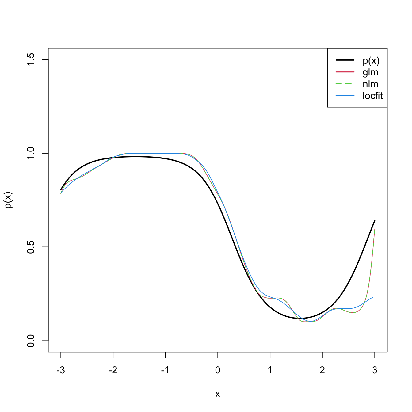

Bandwidth selection can be done by means of likelihood cross-validation. The objective is to maximize the local likelihood fit at $(x_i,Y_i)$ but removing the influence by the datum itself. That is, maximizing

\[\begin{align} \mathrm{LCV}(h)=\sum_{i=1}^n\ell(Y_i,\hat\eta_{-i}(X_i)),\tag{6.34} \end{align}\]

where $\hat\eta_{-i}(x_i)$ represents the local fit at $x_i$ without the $i$-th datum $(x_i,Y_i).$ Unfortunately, the nonlinearity of (6.33) forbids a simplifying result as Proposition 6.1. Thus, in principle,²³⁶ it is required to fit $n$ local likelihoods for sample size $n-1$ for obtaining a single evaluation of (6.34).

We conclude by illustrating how to compute the LCV function and optimize it (keep in mind that much more efficient implementations are possible!).

# Exact LCV -- recall that we *maximize* the LCV!
h <- seq(0.1, 2, by = 0.1)
suppressWarnings(
  LCV <- sapply(h, function(h) {
  sum(sapply(1:n, function(i) {
    K <- dnorm(x = X[i], mean = X[-i], sd = h)
    nlm(f = function(beta) {
      -sum(K * (Y[-i] * (beta[1] + beta[2] * (X[-i] - X[i])) -
                  log(1 + exp(beta[1] + beta[2] * (X[-i] - X[i])))))
      }, p = c(0, 0))$minimum
    }))
  })
)
plot(h, LCV, type = "o")
abline(v = h[which.max(LCV)], col = 2)

References

Aitchison, J., and C. G. G. Aitken. 1976. “Multivariate Binary Discrimination by the Kernel Method.” Biometrika 63 (3): 413–20. https://doi.org/10.1093/biomet/63.3.413.

Chacón, J. E., and T. Duong. 2018. Multivariate Kernel Smoothing and Its Applications. Vol. 160. Monographs on Statistics and Applied Probability. Boca Raton: CRC Press. https://doi.org/10.1201/9780429485572.

Fan, J., and I. Gijbels. 1996. Local Polynomial Modelling and Its Applications. Vol. 66. Monographs on Statistics and Applied Probability. London: Chapman & Hall. https://doi.org/10.2307/2670134.

Li, Q., and J. S. Racine. 2007. Nonparametric Econometrics. Princeton: Princeton University Press. https://press.princeton.edu/books/hardcover/9780691121611/nonparametric-econometrics.

Liu, R. Y. 1988. “Bootstrap Procedures Under Some Non-i.i.d. Models.” The Annals of Statistics 16 (4): 1696–1708. https://doi.org/10.1214/aos/1176351062.

Loader, C. 1999. Local Regression and Likelihood. Statistics and Computing. New York: Springer. https://doi.org/10.2307/1270956.

Marron, J. S., and M. P. Wand. 1992. “Exact Mean Integrated Squared Error.” The Annals of Statistics 20 (2): 712–36. https://doi.org/10.1214/aos/1176348653.

Nadaraya, E. A. 1964. “On Estimating Regression.” Teoriya Veroyatnostei i Ee Primeneniya 9 (1): 157–59. https://doi.org/10.1137/1109020.

Parzen, E. 1962. “On Estimation of a Probability Density Function and Mode.” Annals of Mathematical Statistics 33 (3): 1065–76. https://doi.org/10.1214/aoms/1177704472.

Rosenblatt, M. 1956. “Remarks on Some Nonparametric Estimates of a Density Function.” Annals of Mathematical Statistics 27 (3): 832–37. https://doi.org/10.1214/aoms/1177728190.

Sheather, S. J., and M. C. Jones. 1991. “A Reliable Data-Based Bandwidth Selection Method for Kernel Density Estimation.” Journal of the Royal Statistical Society, Series B (Methodological) 53 (3): 683–90. https://doi.org/10.1111/j.2517-6161.1991.tb01857.x.

Wand, M. P., and M. C. Jones. 1995. Kernel Smoothing. Vol. 60. Monographs on Statistics and Applied Probability. London: Chapman & Hall. https://doi.org/10.1007/978-1-4899-4493-1.

Watson, G. S. 1964. “Smooth Regression Analysis.” Sankhyā, Series A 26 (4): 359–72. https://www.jstor.org/stable/25049340.

For example, linear models assume that $m$ is of the form $m(\mathbf{x})=\beta_0+\beta_1x_1+\cdots+\beta_px_p$ for some unknown coefficients $\boldsymbol{\beta}.$↩︎
For the sake of introducing the main concepts, on Section 6.3 we will see the full general situation.↩︎
Recall that with this standardization we approach to the probability density concept.↩︎
Note that the function has $2n$ discontinuities that are located at $X_i\pm h.$↩︎
$\mathbb{E}[\mathrm{B}(N,p)]=Np$ and $\mathbb{V}\mathrm{ar}[\mathrm{B}(N,p)]=Np(1-p).$↩︎
Or, in other words, if $h^{-1}$ grows slower than $n.$↩︎
Also known as the Parzen–Rosenblatt estimator to honor the proposals by Parzen (1962) and Rosenblatt (1956).↩︎
Although the efficiency of the normal kernel, with respect to the Epanechnikov kernel, is roughly $0.95.$↩︎
Precisely, the rule-of-thumb given by bw.nrd.↩︎
By solving $\frac{\mathrm{d}}{\mathrm{d} h}\mathrm{AMISE}[\hat{f}(\cdot;h)]=0,$ i.e., $\mu_2^2(K)R(f'')h^3- R(K)n^{-1}h^{-2}=0,$ yields $h_\mathrm{AMISE}.$↩︎
Not to confuse with bw.nrd0!↩︎
The motivation for doing so is to try to add the parametric assumption at a later, less important, step.↩︎
Long intervals containing the solution may lead to unsatisfactory termination of the search; short intervals might not contain the minimum.↩︎
But be careful not expanding the upper limit of the search interval too much!↩︎
Observe that, if $p=1,$ then $\mathbf{H}$ will equal the square of the bandwidth $h,$ that is, $\mathbf{H}=h^2.$↩︎
Observe that implementing the optimization of (6.11) is not trivial, since it is required to enforce the constraint $\mathbf{H}\in\mathrm{SPD}_p.$ A neat way of parametrizing $\mathbf{H}$ that induces the positive definiteness constrain is through the (unique) Cholesky decomposition of $\mathbf{H}\in\mathrm{SPD}_p$: $\mathbf{H}=\mathbf{R}^\top\mathbf{R},$ where $\mathbf{R}$ is a triangular matrix with positive entries on the diagonal (but the remaining entries unconstrained). Therefore, optimization of (6.11) can be done through the $\frac{p(p+1)}{2}$ entries of $\mathbf{R}.$↩︎
Notice that it does not depend on $h_2,$ only on $h_1,$ the bandwidth employed for smoothing $X.$↩︎
Termed due to the contemporaneous proposals by Nadaraya (1964) and Watson (1964).↩︎
Obviously, avoiding the spurious perfect fit attained with $\hat{m}(X_i):=Y_i,$ $i=1,\ldots,n.$↩︎
Here we employ $p$ for denoting the order of the Taylor expansion and, correspondingly, the order of the associated polynomial fit. Do not confuse $p$ with the number of original predictors for explaining $Y$ – there is only one predictor in this section, $X.$ However, with a local polynomial fit we expand this predictor to $p$ predictors based on $(X^1,X^2,\ldots,X^p).$↩︎
The rationale is simple: $(X_i,Y_i)$ should be more informative about $m(x)$ than $(X_j,Y_j)$ if $x$ and $X_i$ are closer than $x$ and $X_j.$ Observe that $Y_i$ and $Y_j$ are ignored in measuring this proximity.↩︎
Recall that weighted least squares already appeared in the IRLS of Section 5.2.2.↩︎
Recall that the entries of $\hat{\boldsymbol{\beta}}_h$ are estimating $\boldsymbol{\beta}=\left(m(x), m'(x),\frac{m'(x)}{2},\ldots,\frac{m^{(p)}(x)}{p!}\right)^\top,$ so we are indeed estimating $m(x)$ (first entry) and, in addition, its derivatives up to order $p$!↩︎
The lowess estimator, related with loess, is the one employed in R’s panel.smooth, which is the function in charge of displaying the smooth fits in lm and glm regression diagnostics. For those diagnostics, it employs a prefixed and not data-driven smoothing span of $2/3$ – which makes it inevitably a bad choice for certain data patterns. An example of data pattern for which the span $2/3$ is not appropriate is the one in upper right panel in Figure 5.15.↩︎
We do not address the analysis of the general case in which $p\geq1.$ The reader is referred to, e.g., Theorem 3.1 of Fan and Gijbels (1996) for the full analysis.↩︎
Recall that these are the only assumptions done so far in the model! Compared with the ones made for linear models or generalized linear models, they are extremely mild.↩︎
This assumption requires certain smoothness of the regression function, allowing thus for Taylor expansions to be performed. This assumption is important in practice: $\hat{m}(\cdot;p,h)$ is infinitely differentiable if the considered kernels $K$ are.↩︎
Avoids the situation in which $Y$ is a degenerated random variable.↩︎
Avoids the degenerate situation in which $m$ is estimated at regions without observations of the predictors (such as holes in the support of $X$).↩︎
Meaning that there exist a positive lower bound for $f.$↩︎
Mild assumption inherited from the kde.↩︎
Key assumption for reducing the bias and variance of $\hat{m}(\cdot;p,h)$ simultaneously.↩︎
The notation $o_\mathbb{P}(a_n)$ stands for a random variable that converges in probability to zero at a rate faster than $a_n\to0.$ It is mostly employed for denoting non-important terms in asymptotic expansions, like the ones in (6.24)–(6.25).↩︎
Recall that this makes perfect sense: low density regions of $X$ imply less information about $m$ available.↩︎
The same happened in the linear model with the error variance $\sigma^2.$↩︎
The variance of an unweighted mean is reduced by a factor $n^{-1}$ when $n$ observations are employed. For computing $\hat{m}(x;p,h),$ $n$ observations are used but in a weighted fashion that roughly amounts to considering $nh$ unweighted observations.↩︎
Further details are available in Section 5.8 of Wand and Jones (1995) and references therein.↩︎
A fit based on ordinal polynomial fits but done in different blocks of the data.↩︎
Recall that $h$ is a tuning parameter!↩︎
Indeed, for any other linear smoother of the response, the result also holds.↩︎
Now $q$ denotes the order of the polynomial fit since $p$ stands for the number of predictors.↩︎
In particular, the consideration of Taylor expansions of $m:\mathbb{R}^p\rightarrow\mathbb{R}$ of more than two orders that involve the consideration of the vector of partial derivatives $\mathrm{D}^{\otimes s}m(\mathbf{x})$ formed by $\frac{\partial^s m(\mathbf{x})}{\partial x_1^{s_1}\cdots \partial x_p^{s_1}},$ where $s=s_1+\cdots+s_p.$ For example: if $s=1,$ then $\mathrm{D}^{\otimes 1}m(\mathbf{x})$ is just the transpose of the gradient $\nabla m(\mathbf{x})^\top;$ if $s=2,$ then $\mathrm{D}^{\otimes 2}m(\mathbf{x})$ is the column stacking of the Hessian matrix $\mathcal{H}m(\mathbf{x});$ and if $s\geq3$ the arrangement of derivatives is made in terms of tensors containing the derivatives $\frac{\partial^s m(\mathbf{x})}{\partial x_1^{s_1}\cdots \partial x_p^{s_1}}.$↩︎
The gradient $\nabla m(\mathbf{x})=\left(\frac{\partial m(\mathbf{x})}{\partial x_1},\ldots,\frac{\partial m(\mathbf{x})}{\partial x_p}\right)$ is a row vector.↩︎
Recall that now the entries of $\hat{\boldsymbol{\beta}}_\mathbf{h}$ are estimating $\boldsymbol{\beta}=\left(m(\mathbf{x}), \nabla m(\mathbf{x})\right)^\top.$↩︎
Recall $K_h(x-X_i).$↩︎
Precisely, the ones associated with the asymptotic normality of $\hat{m}(\mathbf{x};p,\mathbf{h})$ and that are based on the results of Theorem 6.1.↩︎
If $p=1,$ then we have the usual simple logistic model.↩︎
No analytical solution for the optimization problem, numerical optimization is needed.↩︎
The interested reader is referred to Sections 4.3.3 and 4.4.3 of Loader (1999) for an approximation of (6.34) that only requires a local likelihood fit for a single sample.↩︎

5 Generalized linear models

A Informal review on hypothesis testing