5 Confidence intervals

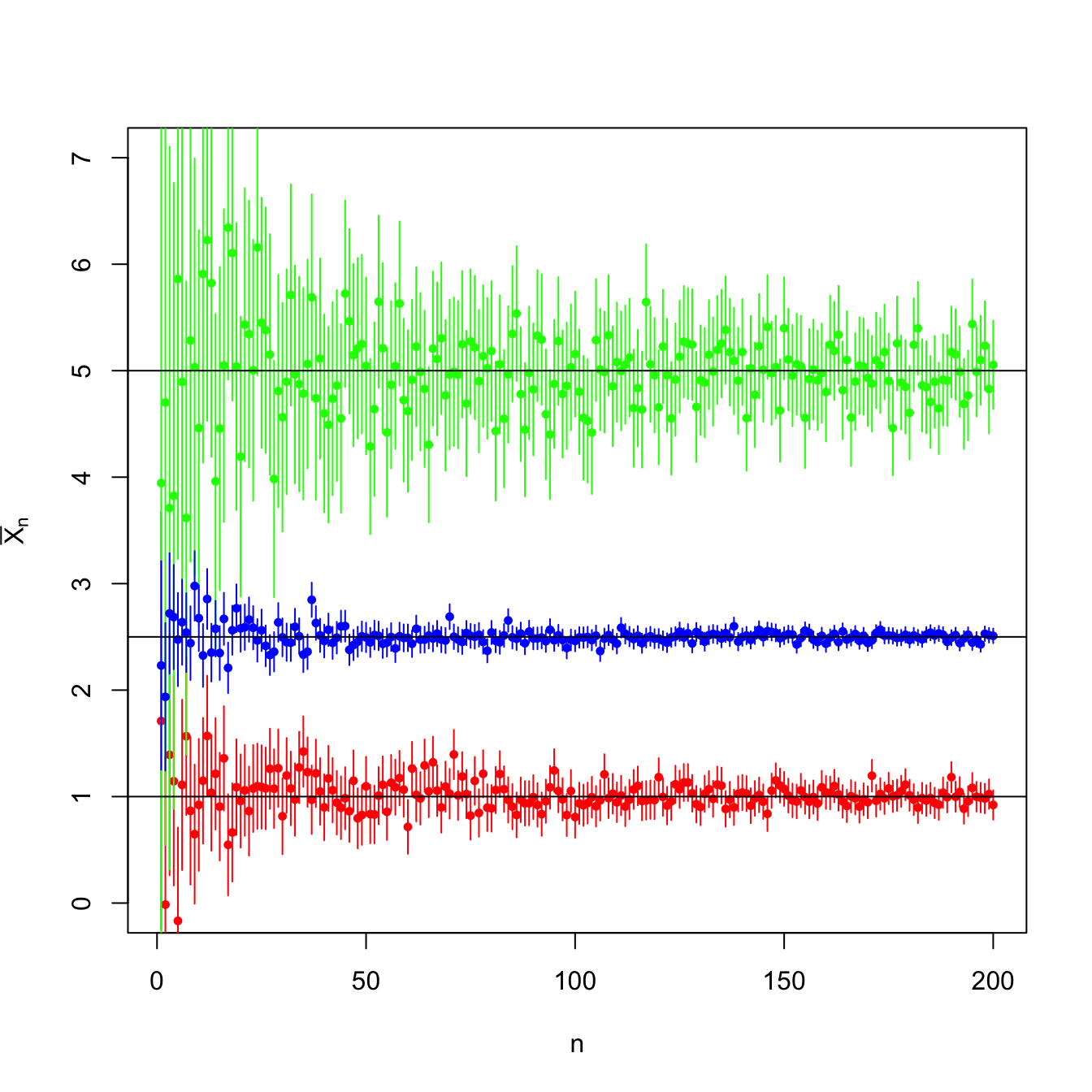
$Evolution of $95\%$-confidence intervals (vertical segments) for the mean $\mu$ constructed from the sample mean $\bar{X}_n$ in a $\mathcal{N}(\mu,\sigma^2)$ population with $(\mu,\sigma^2)\in\{(-2,0.5),(0,3),(2,1)\}.$ For each set of parameters, $N=10$ srs’s of sizes increasing until $n=200$ were simulated. As $n$ grows, the confidence intervals shorten, irrespective of the value of $\sigma^2.$ The confidence intervals contain most of the time the parameter $\mu$ (black horizontal lines). A new sample is generated for each $n$.$

Figure 5.1: Evolution of $95\%$-confidence intervals (vertical segments) for the mean $\mu$ constructed from the sample mean $\bar{X}_n$ in a $\mathcal{N}(\mu,\sigma^2)$ population with $(\mu,\sigma^2)\in\{(-2,0.5),(0,3),(2,1)\}.$ For each set of parameters, $N=10$ srs’s of sizes increasing until $n=200$ were simulated. As $n$ grows, the confidence intervals shorten, irrespective of the value of $\sigma^2.$ The confidence intervals contain most of the time the parameter $\mu$ (black horizontal lines). A new sample is generated for each $n$.

Confidence intervals are the main tools in statistical inference for quantifying and summarizing the uncertainty behind an estimation. In this chapter we introduce the principles of confidence intervals, elaborate on their specifics for the suite of normal populations, and see their applicability in more general settings through the use of asymptotic approximations.

5.1 The pivotal quantity method

Definition 5.1 (Confidence interval) Let $X$ be a rv with induced probability $\mathbb{P}(\cdot;\theta),$ $\theta\in \Theta,$ where $\Theta\subset \mathbb{R}.$ Let $(X_1,\ldots,X_n)$ be a srs of $X.$ Let $T_1=T_1(X_1,\ldots,X_n)$ and $T_2=T_2(X_1,\ldots,X_n)$ be two unidimensional statistics such that

\[\begin{align} \mathbb{P}(T_1\leq \theta\leq T_2;\theta)\geq 1-\alpha, \quad \forall \theta\in\Theta.\tag{5.1} \end{align}\]

Then, the interval $\mathrm{CI}_{1-\alpha}(\theta):=[T_1(x_1,\ldots,x_n),T_2(x_1,\ldots,x_n)]$ obtained for any sample realization $(x_1,\ldots,x_n)$ is referred to as a confidence interval for $\theta$ at the confidence level $1-\alpha$.

The value $\alpha$ is denoted as the significance level. $T_1$ and $T_2$ are known as the inferior and the superior limits of the confidence interval for $\theta,$ respectively. Sometimes the interest lies in only one of these limits.

Definition 5.2 (Pivot) A pivot $Z(\theta)\equiv Z(\theta;X_1,\ldots,X_n)$ is a function of the sample $(X_1,\ldots,X_n)$ and the unknown parameter $\theta$ that is bijective in $\theta$ and has a completely known distribution.

The pivotal quantity method for obtaining a confidence interval consists in, once fixed the significance level $\alpha$ desired to satisfy (5.1), find a pivot $Z(\theta)$ and, using the pivot’s distribution, select two constants $c_1$ and $c_2$ such that

\[\begin{align} \mathbb{P}_Z(c_1\leq Z(\theta)\leq c_2)\geq 1-\alpha. \tag{5.2} \end{align}\]

Then, solving⁶⁰ for $\theta$ in the inequalities we obtain an equivalent probability to (5.2). If $\theta\mapsto Z(\theta)$ is increasing, then (5.2) equals

\[\begin{align*} \mathbb{P}_Z(Z^{-1}(c_1)\leq \theta \leq Z^{-1}(c_2))\geq 1-\alpha, \end{align*}\]

so $T_1=Z^{-1}(c_1)$ and $T_2=Z^{-1}(c_2).$ If $Z$ is decreasing, then $T_1=Z^{-1}(c_2)$ and $T_2=Z^{-1}(c_1).$ In any case, $[T_1,T_2]$ is a confidence interval for $\theta$ at confidence level $1-\alpha.$

Usually, the pivot $Z(\theta)$ can be constructed from an estimator $\hat{\theta}$ of $\theta.$ Assume that making a transformation of the estimator $\hat{\theta}$ that involves $\theta$ we obtain $\hat{\theta}'.$ If the distribution of $\hat{\theta}'$ does not depend on $\theta,$ then we have that $\hat{\theta}'$ is a pivot for $\theta.$ For this process to work, it is key that $\hat{\theta}$ has a known distribution⁶¹ that depends on $\theta$: otherwise the constants $c_1$ and $c_2$ in (5.2) are not computable in practice.

The interpretation of confidence intervals has to be done with a certain care. Notice that in (5.1) the probability operator refers to the randomness of the interval $[T_1,T_2].$ This random confidence interval is said to contain the unknown parameter $\theta$ “with a probability of $1-\alpha$”. Yet, in reality, either $\theta$ belongs to the interval or it does not, which seems contradictory. The previous quoted statement must be understood in the frequentist sense of probability:⁶² when the confidence intervals are computed independently over an increasing number of samples,⁶³ the relative frequency of the event “$\theta\in\mathrm{CI}_{1-\alpha}(\theta)$” converges to $1-\alpha.$ For example, suppose you have 100 samples generated according to a certain distribution model depending on $\theta.$ If you compute $\mathrm{CI}_{1-\alpha}(\theta)$ for each of the samples, then in approximately $100(1-\alpha)$ of the samples the true parameter $\theta$ would actually be inside the random confidence interval. This is illustrated in Figure 5.2.

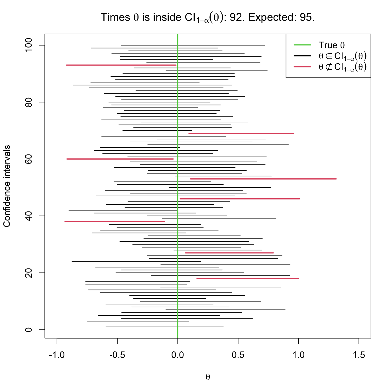
$Illustration of the randomness of the confidence interval for $\theta$ at the $1-\alpha$ confidence. The plot shows 100 random confidence intervals for $\theta,$ computed from 100 random samples generated by the same distribution model (depending on $\theta$).$

Figure 5.2: Illustration of the randomness of the confidence interval for $\theta$ at the $1-\alpha$ confidence. The plot shows 100 random confidence intervals for $\theta,$ computed from 100 random samples generated by the same distribution model (depending on $\theta$).

Example 5.1 Assume that we have a single observation $X$ of a $\mathrm{Exp}(1/\theta)$ rv. Employ $X$ to construct a confidence interval for $\theta$ with a confidence level $0.90.$

We have a srs of size one and we need to find a pivot for $\theta,$ that is, a function of $X$ and $\theta$ whose distribution is completely known. The pdf and the mgf of $X$ are given by

\[\begin{align*} f_X(x)=\frac{1}{\theta}e^{-x/\theta}, \quad x>0, \quad m_X(s)=(1-\theta s)^{-1}. \end{align*}\]

Then, taking $Z=X/\theta,$ the mgf of $Z$ is

\[\begin{align*} m_Z(s)=m_{X/\theta}(s)=m_X(s/\theta)=\left(1-\theta\frac{s}{\theta}\right)^{-1}=(1-s)^{-1}. \end{align*}\]

Therefore, $m_Z$ does not depend on $\theta$ and, in addition, is the mgf of a rv $\mathrm{Exp}(1)$ with pdf

\[\begin{align*} f_Z(z)=e^{-z}, \quad z> 0. \end{align*}\]

Then, we need to find two constants $c_1$ and $c_2$ such that

\[\begin{align*} \mathbb{P}(c_1\leq Z\leq c_2)\geq 0.90. \end{align*}\]

We know that

\[\begin{align*} \mathbb{P}(Z\leq c_1)&=\int_{0}^{c_1} e^{-z}\,\mathrm{d}z=1-e^{-c_1},\\ \mathbb{P}(Z\geq c_2)&=\int_{c_2}^{\infty} e^{-z}\,\mathrm{d}z=e^{-c_2}. \end{align*}\]

Splitting the probability $0.10$ evenly in two,⁶⁴ then

\[\begin{align*} 1-e^{-c_1}=0.05, \quad e^{-c_2}=0.05. \end{align*}\]

Solving for the $c_1$ and $c_2,$ we obtain

\[\begin{align*} c_1=-\log(0.95)\approx0.051,\quad c_2=-\log(0.05)\approx2.996. \end{align*}\]

Therefore, it is verified

\[\begin{align*} \mathbb{P}(c_1\leq X/\theta\leq c_2)= 0.9. \end{align*}\]

Solving $\theta$ from the inequalities, we have

\[\begin{align*} \mathbb{P}(X/2.996\leq \theta\leq X/0.051)\approx 0.9, \end{align*}\]

so the confidence interval for $\theta$ at significance level $0.10$ is

\[\begin{align*} \mathrm{CI}_{0.90}(\theta)\approx[X/2.996,X/0.051]. \end{align*}\]

5.2 Confidence intervals on a normal population

We assume in this section the rv $X$ follows a $\mathcal{N}(\mu,\sigma^2)$ distribution from which a srs $(X_1,\ldots,X_n)$ is extracted. The confidence intervals derived in this section arise from the sampling distributions obtained in Section 2.2 for normal populations. We will apply the pivotal quantity method repeatedly to these sampling distributions.

5.2.1 Confidence interval for the mean with known variance

Let us fix the significance level $\alpha.$ For applying the pivotal quantity method we need an estimator of $\mu$ with known distribution. For example, $\hat{\mu}=\bar{X},$ which verifies

\[\begin{align*} \bar{X}\sim\mathcal{N}\left(\mu,\frac{\sigma^2}{n}\right). \end{align*}\]

A transformation that removes $\mu$ from the distribution of $\bar{X}$ is simply

\[\begin{align*} \bar{X}-\mu\sim\mathcal{N}\left(0,\frac{\sigma^2}{n}\right). \end{align*}\]

However, a more practical pivot is

\[\begin{align} Z:=\frac{\bar{X}-\mu}{\sigma/\sqrt{n}}\sim\mathcal{N}(0,1) \tag{5.3} \end{align}\]

since its distribution is “clean” and does not depend on $\sigma.$

Now we must find the constants $c_1$ and $c_2$ such that

\[\begin{align*} \mathbb{P}(c_1\leq Z\leq c_2)=1-\alpha. \end{align*}\]

If we split the probability $\alpha$ evenly at both sides of the distribution,⁶⁵ then $c_1$ and $c_2$ are the constants that verify

\[\begin{align} \Phi(c_1)=\alpha/2\quad \text{and} \quad \Phi(c_2)=1-\alpha/2, \tag{5.4} \end{align}\]

that is, $c_1$ is the lower $\alpha/2$-quantile of $\mathcal{N}(0,1)$ and $c_2$ is the lower $(1-\alpha/2)$-quantile of the same distribution. $c_1$ and $c_2$ are known as critical values.

Definition 5.3 (Critical value) A critical value $\alpha$ of a continuous⁶⁶ rv $X$ is the value of the variable that accumulates $\alpha$ probability to its right, or in other words, is the upper $\alpha$-quantile of $X.$ It is denoted by $x_{\alpha}$ and is such that

\[\begin{align*} \mathbb{P}(X\geq x_{\alpha})=\alpha. \end{align*}\]

The constants $c_1$ and $c_2$ verify

\[\begin{align*} \mathbb{P}(Z\geq c_1)=1-\alpha/2\quad \text{and} \quad \mathbb{P}(Z\geq c_2)=\alpha/2, \end{align*}\]

that is, $c_1=z_{1-\alpha/2}$ and $c_2=z_{\alpha/2}.$ Given the symmetry of the standard normal distribution with respect to $0,$ it is verified that $z_{1-\alpha/2}=-z_{\alpha/2},$ that is, $c_1=-c_2.$ Example 2.8 illustrated how to compute the critical values of a $\mathcal{N}(0,1)$ in R. In terms of the cdf $\Phi$ of $\mathcal{N}(0,1),$ and connecting with (5.4), we have

\[\begin{align*} \Phi(z_{1-\alpha/2})=\Phi(-z_{\alpha/2})=\alpha/2\quad \text{and} \quad \Phi(z_{\alpha/2})=1-\alpha/2. \end{align*}\]

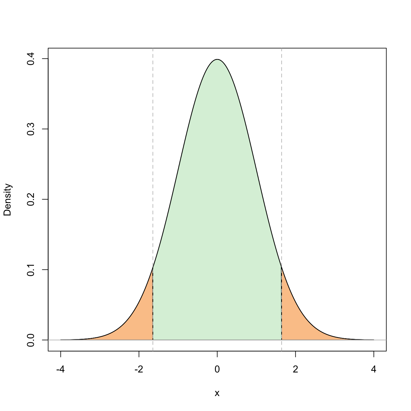
$Representation of the probability $\mathbb{P}(-z_{\alpha/2}\leq Z\leq z_{\alpha/2})=1-\alpha$ (in green) and its complementary (in orange) for $\alpha=0.10$.$

Figure 5.3: Representation of the probability $\mathbb{P}(-z_{\alpha/2}\leq Z\leq z_{\alpha/2})=1-\alpha$ (in green) and its complementary (in orange) for $\alpha=0.10$.

Once obtained $c_1=-z_{\alpha/2}$ and $c_2=z_{\alpha/2},$ we solve for $\mu$ in the inequalities inside the probability:

\[\begin{align*} 1-\alpha &=\mathbb{P}\left(-z_{\alpha/2}\leq \frac{\bar{X}-\mu}{\sigma/\sqrt{n}}\leq z_{\alpha/2}\right)\\ &=\mathbb{P}\left(-z_{\alpha/2}\frac{\sigma}{\sqrt{n}}\leq \bar{X}-\mu\leq z_{\alpha/2}\frac{\sigma}{\sqrt{n}}\right)\\ &=\mathbb{P}\left(-\bar{X}-z_{\alpha/2}\frac{\sigma}{\sqrt{n}}\leq -\mu\leq -\bar{X}+z_{\alpha/2}\frac{\sigma}{\sqrt{n}}\right) \\ &=\mathbb{P}\left(\bar{X}-z_{\alpha/2}\frac{\sigma}{\sqrt{n}}\leq \mu\leq \bar{X}+z_{\alpha/2}\frac{\sigma}{\sqrt{n}}\right). \end{align*}\]

Therefore, a confidence interval for $\mu$ is

\[\begin{align*} \mathrm{CI}_{1-\alpha}(\mu)=\left[\bar{X}-z_{\alpha/2}\frac{\sigma}{\sqrt{n}}, \bar{X}+z_{\alpha/2}\frac{\sigma}{\sqrt{n}}\right]. \end{align*}\]

We represent it in a compact way as

\[\begin{align*} \mathrm{CI}_{1-\alpha}(\mu)=\left[\bar{X}\mp z_{\alpha/2}\frac{\sigma}{\sqrt{n}}\right]. \end{align*}\]

Example 5.2 A gunpowder manufacturer developed a new formula that was tested in eight bullets. The resultant initial velocities, measured in meters per second, were

\[\begin{align*} 916, 892, 895, 904, 913, 916, 895, 885. \end{align*}\]

Assuming that the initial velocities have normal distribution with $\sigma=12$ meters per second, find a confidence interval at significance level $\alpha=0.05$ for the initial mean velocity of the bullets that employ the new gunpowder.

We know that

\[\begin{align*} X\sim \mathcal{N}(\mu,12^2), \ \text{with unknown $\mu$}. \end{align*}\]

From the sample we have that

\[\begin{align*} n=8,\quad \bar{X}=902,\quad \alpha/2=0.025, \quad z_{\alpha/2}\approx1.96. \end{align*}\]

Then, a confidence interval for $\mu$ at $0.95$ confidence is

\[\begin{align*} \mathrm{CI}_{0.95}(\mu)=\left[\bar{X}\mp z_{\alpha/2}\frac{\sigma}{\sqrt{n}}\right]=\left[902\mp z_{\alpha/2}\frac{12}{\sqrt{8}}\right]\approx[893.68, 910.32]. \end{align*}\]

In R, the previous computations can be simply done as:

# Sample
X <- c(916, 892, 895, 904, 913, 916, 895, 885)

# n, mean, sigma, alpha, z_{\alpha/2}
n <- length(X)
X_bar <- mean(X)
sigma <- 12
alpha <- 0.05
z <- qnorm(alpha / 2, lower.tail = FALSE)

# CI
X_bar + c(-1, 1) * z * sigma / sqrt(n)
## [1] 893.6846 910.3154

5.2.2 Confidence interval for the mean with unknown variance

In this case (5.3) is not a pivot: besides depending on $\mu,$ the statistic also depends on another unknown parameter, $\sigma^2,$ which makes it impossible to encapsulate $\mu$ between two computable limits. However, we can estimate $\sigma^2$ unbiasedly with $S'^2,$ and produce

\[\begin{align*} T:=\frac{\bar{X}-\mu}{S'/\sqrt{n}}. \end{align*}\]

$T$ is a pivot, since Theorem 2.3 provides the $\mu$-free distribution of $T,$ $t_{n-1}.$ If we split evenly the significance level $\alpha$ between the two tails of the distribution, then the constants $c_1$ and $c_2$ are

\[\begin{align*} \mathbb{P}(c_1\leq T\leq c_2)=1-\alpha, \end{align*}\]

corresponding to the critical values $c_1=t_{n-1;1-\alpha/2}$ and $c_2=t_{n-1;\alpha/2}.$ Since Student’s $t$ is also symmetric, then $c_1=-c_2=-t_{n-1;\alpha/2},$ hence

\[\begin{align*} 1-\alpha=\mathbb{P}\left(-t_{n-1;\alpha/2}\leq \frac{\bar{X}-\mu}{S'/\sqrt{n}}\leq t_{n-1;\alpha/2}\right). \end{align*}\]

Example 2.11 illustrated how to compute probabilities in a Student’s $t$ distribution.

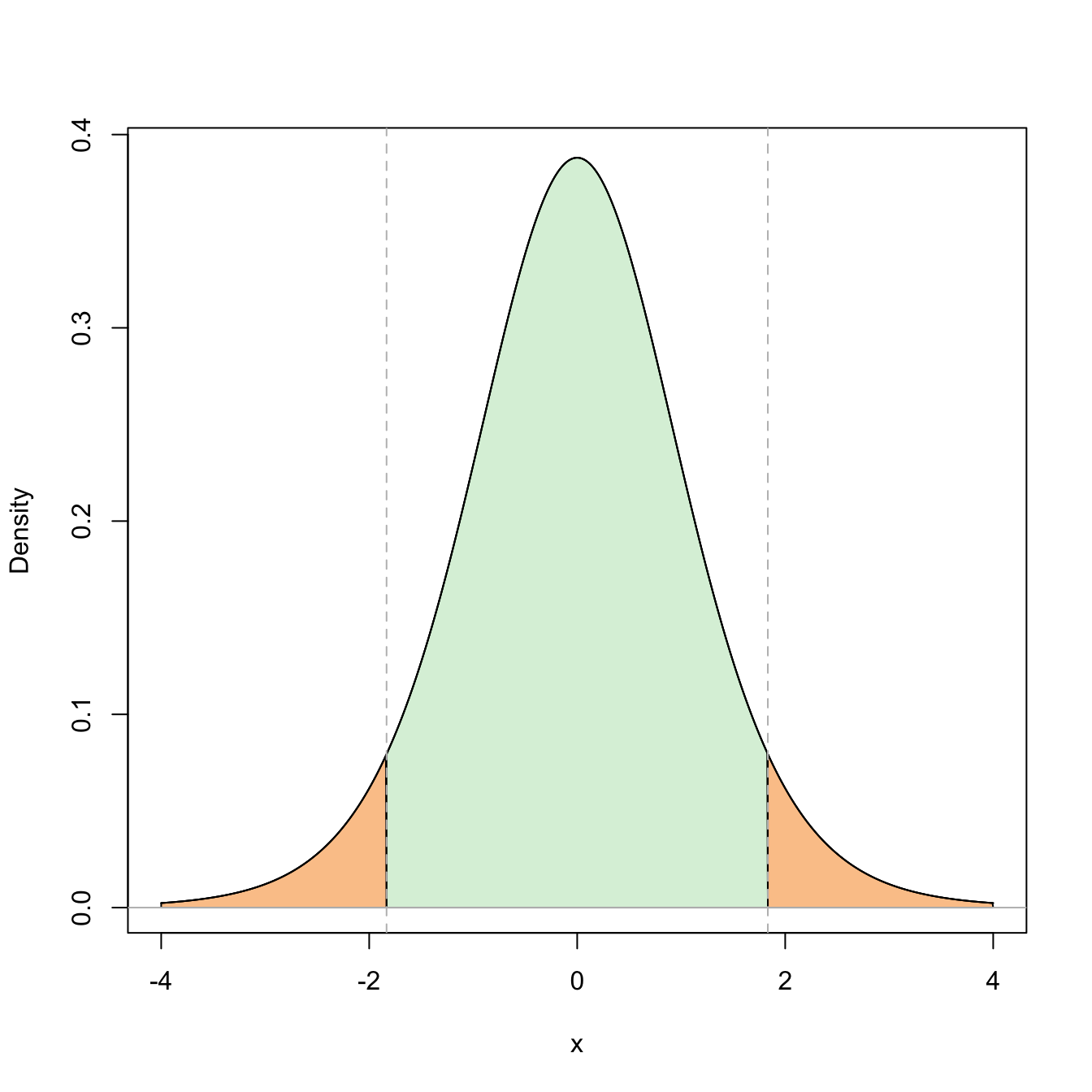
$Representation of the probability $\mathbb{P}(-t_{n-1;\alpha/2}\leq t_{n-1}\leq t_{n-1;\alpha/2})=1-\alpha$ (in green) and its complementary (in orange) for $\alpha=0.10$ and $n=10$.$

Figure 5.4: Representation of the probability $\mathbb{P}(-t_{n-1;\alpha/2}\leq t_{n-1}\leq t_{n-1;\alpha/2})=1-\alpha$ (in green) and its complementary (in orange) for $\alpha=0.10$ and $n=10$.

Solving $\mu$ in the inequalities, we get

\[\begin{align*} 1-\alpha=\mathbb{P}\left(\bar{X}-t_{n-1;\alpha/2}{S'/\sqrt{n}}\leq\mu\leq \bar{X}+t_{n-1;\alpha/2}{S'/\sqrt{n}}\right). \end{align*}\]

Then, a confidence interval for the mean $\mu$ at confidence level $1-\alpha$ is

\[\begin{align*} \mathrm{CI}_{1-\alpha}(\mu)=\left[\bar{X}\mp t_{n-1;\alpha/2}\frac{S'}{\sqrt{n}}\right]. \end{align*}\]

Example 5.3 Compute the same confidence interval asked in the Example 5.2 but assuming that the variance of the initial velocities is unknown.

If the variance is unknown, then we can estimate it with $S'^2=143.43.$ Using $t_{7;0.025}\approx 2.365,$ the confidence interval for $\mu$ is

\[\begin{align*} \mathrm{CI}_{0.95}(\mu)=\left[\bar{X}\mp t_{7;0.025}\frac{S'}{\sqrt{n}}\right]\approx\left[902\mp 2.365\times\sqrt{\frac{143.43}{8}}\right]\approx[891.99, 912.01]. \end{align*}\]

In R, the previous computations can be simply done as:

# Sample
X <- c(916, 892, 895, 904, 913, 916, 895, 885)

# n, mean, S', alpha, t_{\alpha/2;n-1}
n <- length(X)
X_bar <- mean(X)
S_prime <- sd(X)
alpha <- 0.05
t <- qt(alpha / 2, df = n - 1, lower.tail = FALSE)

# CI
X_bar + c(-1, 1) * t * S_prime / sqrt(n)
## [1] 891.9877 912.0123

5.2.3 Confidence interval for the variance

We already have an unbiased estimator of $\sigma^2,$ the quasivariance $S'^2.$ In addition, by Theorem 2.2 we have a pivot

\[\begin{align*} U:=\frac{(n-1)S'^2}{\sigma^2}\sim \chi_{n-1}^2. \end{align*}\]

Then, we only need to compute the constants $c_1$ and $c_2$ such that

\[\begin{align*} \mathbb{P}(c_1\leq U\leq c_2)=1-\alpha. \end{align*}\]

Splitting the probability $\alpha$ evenly to both sides of the $\chi^2$ distribution,⁶⁷ we have that $c_1=\chi_{n-1;1-\alpha/2}^2$ and $c_2=\chi_{n-1;\alpha/2}^2.$ Once the constants are computed, solving for $\sigma^2$ in the inequalities

\[\begin{align*} 1-\alpha &=\mathbb{P}\left(\chi_{n-1;1-\alpha/2}^2\leq \frac{(n-1)S'^2}{\sigma^2} \leq \chi_{n-1;\alpha/2}^2\right)\\ &=\mathbb{P}\left(\frac{\chi_{n-1;1-\alpha/2}^2}{(n-1)S'^2}\leq \frac{1}{\sigma^2} \leq \frac{\chi_{n-1;\alpha/2}^2}{(n-1)S'^2}\right) \\ &=\mathbb{P}\left(\frac{(n-1)S'^2}{\chi_{n-1;\alpha/2}^2}\leq \sigma^2 \leq \frac{(n-1)S'^2}{\chi_{n-1;1-\alpha/2}^2}\right) \end{align*}\]

yields the confidence interval for $\sigma^2$:

\[\begin{align*} \mathrm{CI}_{1-\alpha}(\sigma^2)=\left[\frac{(n-1)S'^2}{\chi_{n-1;\alpha/2}^2}, \frac{(n-1)S'^2}{\chi_{n-1;1-\alpha/2}^2}\right]. \end{align*}\]

Observe that $\chi_{n-1;1-\alpha/2}^2<\chi_{n-1;\alpha/2}^2$ but in the confidence interval these critical values appear in the denominators in reverse order.

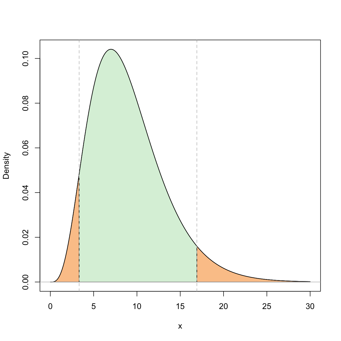
$Representation of the probability $\mathbb{P}(\chi^2_{n-1;1-\alpha/2}\leq \chi^2_{n-1}\leq \chi^2_{n-1;\alpha/2})=1-\alpha$ (in green) and its complementary (in orange) for $\alpha=0.10$ and $n=10$.$

Figure 5.5: Representation of the probability $\mathbb{P}(\chi^2_{n-1;1-\alpha/2}\leq \chi^2_{n-1}\leq \chi^2_{n-1;\alpha/2})=1-\alpha$ (in green) and its complementary (in orange) for $\alpha=0.10$ and $n=10$.

Example 5.4 A practitioner wants to verify the variability of an equipment employed for measuring the volume of an audio source. Three independent measurements recorded with this equipment were

\[\begin{align*} 4.1,\quad 5.2, \quad 10.2. \end{align*}\]

Assuming that the measurements have a normal distribution, obtain the confidence interval of $\sigma^2$ with confidence $0.90.$

From the three measurements we obtain

\[\begin{align*} S'^2=10.57,\quad \alpha/2=0.05,\quad n=3. \end{align*}\]

Then, the confidence interval for $\sigma^2$ is

\[\begin{align*} \mathrm{CI}_{0.90}(\sigma^2)=\left[\frac{(n-1)S'^2}{\chi_{2;0.05}^2},\frac{(n-1)S'^2}{\chi_{2;0.95}^2}\right]\approx\left[\frac{2\times 10.57}{5.991},\frac{2\times 10.57}{0.103}\right]\approx[3.53,205.24]. \end{align*}\]

Recall that since $n$ is small, then the critical value $c_1=\chi_{n-1;1-\alpha/2}^2$ of the $\chi_{n-1}^2$ distribution is close to zero (see Figure 5.5), and hence the length of the interval is large, illustrating the little information available.

The previous computations can be done as:

# Sample
X <- c(4.1, 5.2, 10.2)

# n, S'^2, alpha, c1, c2
n <- length(X)
S2_prime <- var(X)
alpha <- 0.10
c1 <- qchisq(1 - alpha / 2, df = n - 1, lower.tail = FALSE)
c2 <- qchisq(alpha / 2, df = n - 1, lower.tail = FALSE)

# CI
(n - 1) * S2_prime / c(c2, c1)
## [1]   3.528353 206.069821

5.3 Confidence intervals on two normal populations

We assume now that we have two independent populations $X_1\sim \mathcal{N}(\mu_1,\sigma_1^2)$ and $X_2\sim \mathcal{N}(\mu_2,\sigma_2^2)$ from which two respective srs’s $(X_{11},\ldots,X_{1n_1})$ and $(X_{21},\ldots,X_{2n_2})$ of sizes $n_1$ and $n_2$ are extracted. As in Section 5.2, the confidence intervals derived in this section arise from the sampling distributions obtained in Section 2.2 for normal populations.

5.3.1 Confidence interval for the difference of means with known variances

Assume that the mean populations $\mu_1$ and $\mu_2$ are unknown and the variances $\sigma_1^2$ and $\sigma_2^2$ are known. We wish to construct a confidence interval for the difference $\theta=\mu_1-\mu_2.$

For that, we consider an estimator of $\theta.$ An unbiased estimator is

\[\begin{align*} \hat{\theta}=\bar{X}_1-\bar{X}_2. \end{align*}\]

Since $\hat{\theta}$ is a linear combination of normal rv’s, then it is normally distributed. Its mean is easily computed as

\[\begin{align*} \mathbb{E}\big[\hat{\theta}\big]=\mathbb{E}[\bar{X}_1]-\mathbb{E}[\bar{X}_2]=\mu_1-\mu_2. \end{align*}\]

Thanks to the independence between $X_1$ and $X_2,$ the variance is⁶⁸

\[\begin{align*} \mathbb{V}\mathrm{ar}\big[\hat{\theta}\big]=\mathbb{V}\mathrm{ar}[\bar{X}_1]+\mathbb{V}\mathrm{ar}[\bar{X}_2]=\frac{\sigma_1^2}{n_1}+\frac{\sigma_2^2}{n_2}. \end{align*}\]

Then, a possible pivot is

\[\begin{align*} Z:=\frac{\bar{X}_1-\bar{X}_2-(\mu_1-\mu_2)}{\sqrt{\frac{\sigma_1^2}{n_1}+\frac{\sigma_2^2}{n_2}}}\sim\mathcal{N}(0,1). \end{align*}\]

Again, if we split evenly the significance level $\alpha$ between the two tails, then we look for constants $c_1$ and $c_2$ such that

\[\begin{align*} \mathbb{P}(c_1\leq Z\leq c_2)=1-\alpha, \end{align*}\]

that is, $c_1=-z_{\alpha/2}$ and $c_2=z_{\alpha/2}.$ Solving for $\mu_1-\mu_2,$ we obtain

\[\begin{align*} 1-\alpha &=\mathbb{P}\left(-z_{\alpha/2}\leq \frac{\bar{X}_1-\bar{X}_2-(\mu_1-\mu_2)}{\sqrt{\frac{\sigma_1^2}{n_1}+\frac{\sigma_2^2}{n_2}}}\leq z_{\alpha/2}\right) \\ &=\mathbb{P}\left(-z_{\alpha/2}\sqrt{\frac{\sigma_1^2}{n_1}+\frac{\sigma_2^2}{n_2}}\leq \bar{X}_1-\bar{X}_2-(\mu_1-\mu_2)\leq z_{\alpha/2}\sqrt{\frac{\sigma_1^2}{n_1}+\frac{\sigma_2^2}{n_2}}\right)\\ &=\mathbb{P}\left(-(\bar{X}_1-\bar{X}_2)-z_{\alpha/2}\sqrt{\frac{\sigma_1^2}{n_1}+\frac{\sigma_2^2}{n_2}}\leq -(\mu_1-\mu_2)\leq -(\bar{X}_1-\bar{X}_2)+z_{\alpha/2}\sqrt{\frac{\sigma_1^2}{n_1}+\frac{\sigma_2^2}{n_2}}\right)\\ &=\mathbb{P}\left(\bar{X}_1-\bar{X}_2-z_{\alpha/2}\sqrt{\frac{\sigma_1^2}{n_1}+\frac{\sigma_2^2}{n_2}}\leq \mu_1-\mu_2\leq \bar{X}_1-\bar{X}_2+z_{\alpha/2}\sqrt{\frac{\sigma_1^2}{n_1}+\frac{\sigma_2^2}{n_2}}\right). \end{align*}\]

Therefore, a confidence interval for $\mu_1-\mu_2$ at the confidence level $1-\alpha$ is

\[\begin{align*} \mathrm{CI}_{1-\alpha}(\mu_1-\mu_2)=\left[\bar{X}_1-\bar{X}_2 \mp z_{\alpha/2}\sqrt{\frac{\sigma_1^2}{n_1}+\frac{\sigma_2^2}{n_2}}\right]. \end{align*}\]

Example 5.5 A new training method for an assembly operation is being tested at a factory. For that purpose, two groups of nine employees were trained during three weeks. One group was trained with the usual procedure and the other with the new method. The assembly time (in minutes) that each employee required after the training period is collected in the table below. Assuming that the assembly times are normally distributed with both variances equal to $22$ minutes$^2,$ obtain a confidence interval at significance level $0.05$ for the difference of average assembly times for the two kinds of training.

Procedure	Measurements
Standard	$32 \qquad 37 \qquad 35 \qquad 28 \qquad 41 \qquad 44 \qquad 35 \qquad 31 \qquad 34$
New	$35 \qquad 31 \qquad 29 \qquad 25 \qquad 34 \qquad 40 \qquad 27 \qquad 32 \qquad 31$

The average assembly times of the two groups are

\[\begin{align*} \bar{X}_1\approx35.22,\quad \bar{X}_2\approx31.56. \end{align*}\]

Then, a confidence interval for $\mu_1-\mu_2$ at the $0.95$ confidence level is

\[\begin{align*} \mathrm{CI}_{0.95}(\mu_1-\mu_2)&\approx\left[(35.22-31.56)\mp 1.96\times 4.69\sqrt{1/9+1/9}\right]\\ &\approx[3.66\mp 4.33]=[-0.67,7.99]. \end{align*}\]

In R:

# Samples
X_1 <- c(32, 37, 35, 28, 41, 44, 35, 31, 34)
X_2 <- c(35, 31, 29, 25, 34, 40, 27, 32, 31)

# n1, n2, Xbar1, Xbar2, sigma2_1, sigma2_2, alpha, z_{alpha/2}
n_1 <- length(X_1)
n_2 <- length(X_2)
X_bar_1 <- mean(X_1)
X_bar_2 <- mean(X_2)
sigma2_1 <- sigma2_2 <- 22
alpha <- 0.05
z <- qnorm(alpha / 2, lower.tail = FALSE)

# CI
(X_bar_1 - X_bar_2) + c(-1, 1) * z * sqrt(sigma2_1 / n_1 + sigma2_2 / n_2)
## [1] -0.6669768  8.0003101

5.3.2 Confidence interval for the difference of means, with unknown and equal variances

Assume that we are in the situation of the previous section but now both variances $\sigma_1^2$ and $\sigma_2^2$ are equal and unknown, that is, $\sigma_1^2=\sigma_2^2=\sigma^2$ with $\sigma^2$ unknown.

We want to construct a confidence interval for $\theta=\mu_1-\mu_2.$ As in the previous section, an unbiased estimator is

\[\begin{align*} \hat{\theta}=\hat{\mu}_1-\hat{\mu}_2=\bar{X}_1-\bar{X}_2 \end{align*}\]

whose distribution is

\[\begin{align*} \hat{\theta}\sim\mathcal{N}\left(\mu_1-\mu_2,\sigma^2\left(\frac{1}{n_1}+\frac{1}{n_2}\right)\right). \end{align*}\]

However, since $\sigma^2$ is unknown, then

\[\begin{align} Z=\frac{\bar{X}_1-\bar{X}_2-(\mu_1-\mu_2)}{\sqrt{\sigma^2\left(\frac{1}{n_1}+\frac{1}{n_2}\right)}}\sim\mathcal{N}(0,1)\tag{5.5} \end{align}\]

is not a pivot. We need to estimate in the first place $\sigma^2.$

For that, we know that

\[\begin{align*} \frac{(n_1-1)S_1'^2}{\sigma^2}\sim \chi_{n_1-1}^2,\quad \frac{(n_2-1)S_2'^2}{\sigma^2}\sim \chi_{n_2-1}^2. \end{align*}\]

Besides, the two samples are independent, so by the additivity property of the $\chi^2$ distribution we know that

\[\begin{align*} \frac{(n_1-1)S_1'^2}{\sigma^2}+\frac{(n_2-1)S_2'^2}{\sigma^2}\sim \chi_{n_1+n_2-2}^2. \end{align*}\]

Taking expectations, we have

\[\begin{align*} \mathbb{E}\left[\frac{(n_1-1)S_1'^2}{\sigma^2}+\frac{(n_2-1)S_2'^2}{\sigma^2}\right] &=\frac{1}{\sigma^2}\mathbb{E}\left[(n_1-1)S_1'^2+(n_2-1)S_2'^2\right]\\ &=n_1+n_2-2. \end{align*}\]

Solving for $\sigma^2,$ we obtain

\[\begin{align*} \mathbb{E}\left[(n_1-1)S_1'^2+(n_2-1)S_2'^2\right]=\sigma^2(n_1+n_2-2). \end{align*}\]

From here we can easily deduce an unbiased estimator for $\sigma^2$:

\[\begin{align*} \hat{\sigma}^2=\frac{(n_1-1)S_1'^2+(n_2-1)S_2'^2}{n_1+n_2-2}=: S^2. \end{align*}\]

Note that $\hat{\sigma}^2$ is just a pooled sample quasivariance stemming from the two sample quasivariances. The weights of each quasivariance are relative to their degrees of freedom. In addition, we know the distribution of $\hat{\sigma}^2,$ since

\[\begin{align*} \frac{(n_1+n_2-2)S^2}{\sigma^2}=\frac{(n_1-1)S_1'^2+(n_2-1)S_2'^2}{\sigma^2}\sim\chi_{n_1+n_2-2}^2. \end{align*}\]

If we replace $\sigma^2$ in (5.5) with $S^2$ and we apply Theorem 2.3, we obtain the probability distribution

\[\begin{align*} T&=\frac{\bar{X}_1-\bar{X}_2-(\mu_1-\mu_2)}{\sqrt{S^2\left(\frac{1}{n_1}+\frac{1}{n_2}\right)}}=\frac{{\frac{\bar{X}_1-\bar{X}_2-(\mu_1-\mu_2)}{\sqrt{\sigma^2\left(\frac{1}{n_1}+\frac{1}{n_2}\right)}}}}{\sqrt{{\frac{(n_1+n_2-2)S^2}{\sigma^2}/(n_1+n_2-2)}}} \\ &\stackrel{d}{=} \frac{\mathcal{N}(0,1)}{\sqrt{\chi_{n_1+n_2-2}^2/(n_1+n_2-2)}}=t_{n_1+n_2-2}. \end{align*}\]

Then, solving $\mu_1-\mu_2$ within the following probability we find a confidence interval for $\mu_1-\mu_2$:

\[\begin{align*} 1-\alpha&=\mathbb{P}\left(-t_{n_1+n_2-2;\alpha/2}\leq \frac{\bar{X}_1-\bar{X}_2-(\mu_1-\mu_2)}{\sqrt{S^2\left(\frac{1}{n_1}+\frac{1}{n_2}\right)}} \leq t_{n_1+n_2-2;\alpha/2}\right)\\ &=\mathbb{P}\left(-t_{n_1+n_2-2;\alpha/2}S\sqrt{\frac{1}{n_1}+\frac{1}{n_2}} \leq \bar{X}_1-\bar{X}_2-(\mu_1-\mu_2) \leq t_{n_1+n_2-2;\alpha/2} S\sqrt{\frac{1}{n_1}+\frac{1}{n_2}} \right)\\ &=\mathbb{P}\left(\bar{X}_1-\bar{X}_2-t_{n_1+n_2-2;\alpha/2}S\sqrt{\frac{1}{n_1}+\frac{1}{n_2}} \leq \mu_1-\mu_2 \leq \bar{X}_1-\bar{X}_2+t_{n_1+n_2-2;\alpha/2} S\sqrt{\frac{1}{n_1}+\frac{1}{n_2}} \right). \end{align*}\]

Therefore, a confidence interval for $\mu_1-\mu_2$ at confidence level $1-\alpha$ is

\[\begin{align*} \mathrm{CI}_{1-\alpha}(\mu_1-\mu_2)=\left[\bar{X}_1-\bar{X}_2\mp t_{n_1+n_2-2;\alpha/2}S\sqrt{\frac{1}{n_1}+\frac{1}{n_2}}\right]. \end{align*}\]

Example 5.6 Compute the same interval asked in Example 5.5, but now assuming that the assembly variances are unknown and equal for the two training methods.

The sample quasivariances for each of the methods are

\[\begin{align*} S_1'^2=195.56/8=24.445,\quad S_2'^2=160.22/8=20.027. \end{align*}\]

Therefore, the pooled estimated variance is

\[\begin{align*} S^2=\frac{8\times 24.445+8\times 20.027}{9+9-2}\approx22.24, \end{align*}\]

and the standard deviation is $S\approx 4.71.$ Then, a confidence interval at confidence level $0.95$ for the difference of average times is

\[\begin{align*} \mathrm{CI}_{0.95}(\mu_1-\mu_2)&\approx\left[(35.22-31.56)\mp t_{16;0.025}\,4.71\sqrt{1/9+1/9}\right]\\ &\approx[3.66\mp 4.71]=[-1.05,8.37]. \end{align*}\]

In R:

# Samples
X_1 <- c(32, 37, 35, 28, 41, 44, 35, 31, 34)
X_2 <- c(35, 31, 29, 25, 34, 40, 27, 32, 31)

# n1, n2, Xbar1, Xbar2, S^2, alpha, t_{alpha/2;n1-n2-2}
n_1 <- length(X_1)
n_2 <- length(X_2)
X_bar_1 <- mean(X_1)
X_bar_2 <- mean(X_2)
S2_prime_1 <- var(X_1)
S2_prime_2 <- var(X_2)
S <- sqrt(((n_1 - 1) * S2_prime_1 + (n_2 - 1) * S2_prime_2) / (n_1 + n_2 - 2))
alpha <- 0.05
t <- qt(alpha / 2, df = n_1 + n_2 - 2, lower.tail = FALSE)

# CI
(X_bar_1 - X_bar_2) + c(-1, 1) * t * S * sqrt(1 / n_1 + 1 / n_2)
## [1] -1.045706  8.379039

5.3.3 Confidence interval for the ratio of variances

Assume that neither the mean nor the variances are known. We wish to construct a confidence interval for the ratio of variances, $\theta=\sigma_1^2/\sigma_2^2.$

In order to find a pivot, we need to consider an estimator for $\theta.$ We know that $S_1'^2$ and $S_2'^2$ are unbiased estimators for $\sigma_1^2$ and $\sigma_2^2,$ respectively. Also, since both srs’s are independent, then so are $S_1'^2$ and $S_2'^2.$ In addition, by Theorem 2.2, we know that

\[\begin{align*} \frac{(n_1-1)S_1'^2}{\sigma_1^2}\sim \chi_{n_1-1}^2, \quad \frac{(n_2-1)S_2'^2}{\sigma_2^2}\sim \chi_{n_2-1}^2. \end{align*}\]

A possible estimator for $\theta$ is $\hat{\theta}=S_1'^2/S_2'^2,$ but its distribution is not completely known, since it depends on $\sigma_1^2$ and $\sigma_2^2.$ However, we do know the distribution of

\[\begin{align*} F=\frac{S_1'^2/\sigma_1^2}{S_2'^2/\sigma_2^2}=\frac{\frac{(n_1-1)S_1'^2}{\sigma_1^2}/(n_1-1)}{\frac{(n_2-1)S_2'^2}{\sigma_2^2}/(n_2-1)}\sim \frac{\chi_{n_1-1}^2/(n_1-1)}{\chi_{n_2-1}^2/(n_2-1)}\stackrel{d}{=}\mathcal{F}_{n_1-1,n_2-1}. \end{align*}\]

Therefore, $F$ is a pivot. Splitting the probability $\alpha$ evenly between both tails of the $\mathcal{F}_{n_1-1,n_2-1}$ distribution and solving for $\theta,$ we get

\[\begin{align*} 1-\alpha &=\mathbb{P}\left(\mathcal{F}_{n_1-1,n_2-1;1-\alpha/2} \leq \frac{S_1'^2/S_2'^2}{\sigma_1^2/\sigma_2^2} \leq \mathcal{F}_{n_1-1,n_2-1;\alpha/2}\right) \\ &=\mathbb{P}\left(\frac{S_2'^2}{S_1'^2}\mathcal{F}_{n_1-1,n_2-1;1-\alpha/2} \leq \frac{1}{\sigma_1^2/\sigma_2^2} \leq \frac{S_2'^2}{S_1'^2}\mathcal{F}_{n_1-1,n_2-1;\alpha/2}\right)\\ &=\mathbb{P}\left(\frac{S_1'^2/S_2'^2}{\mathcal{F}_{n_1-1,n_2-1;\alpha/2}} \leq \frac{\sigma_1^2}{\sigma_2^2} \leq \frac{S_1'^2/S_2'^2}{\mathcal{F}_{n_1-1,n_2-1;1-\alpha/2}}\right). \end{align*}\]

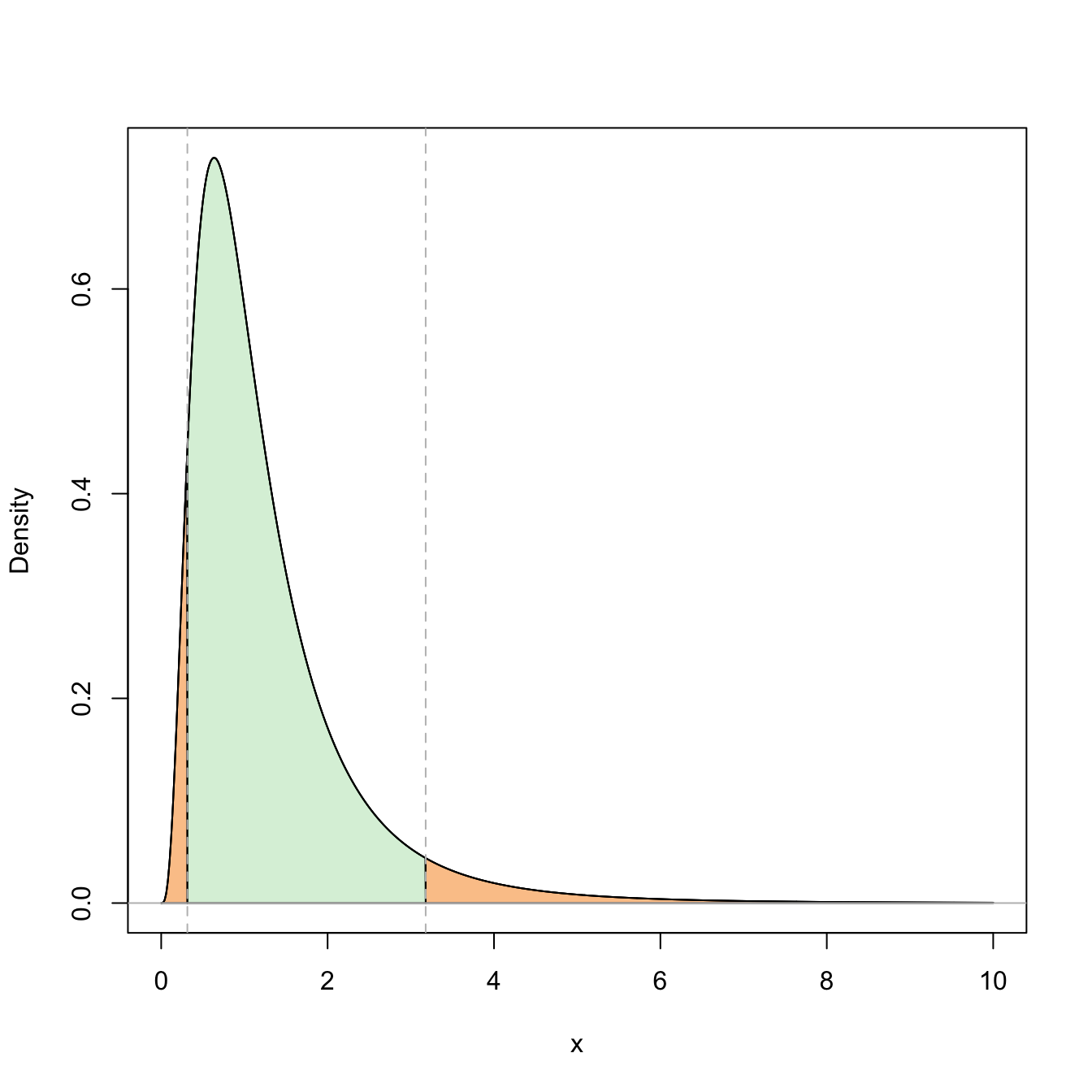
$Representation of the probability $\mathbb{P}(\mathcal{F}_{n_1-1,n_2-1;1-\alpha/2}\leq \mathcal{F}_{n_1-1,n_2-1}\leq \mathcal{F}_{n_1-1,n_2-1;\alpha/2})=1-\alpha$ (in green) and its complementary (in orange) for $\alpha=0.10$ and $n_1=n_2=10$.$

Figure 5.6: Representation of the probability $\mathbb{P}(\mathcal{F}_{n_1-1,n_2-1;1-\alpha/2}\leq \mathcal{F}_{n_1-1,n_2-1}\leq \mathcal{F}_{n_1-1,n_2-1;\alpha/2})=1-\alpha$ (in green) and its complementary (in orange) for $\alpha=0.10$ and $n_1=n_2=10$.

Then, a confidence interval for $\theta=\sigma_1^2/\sigma_2^2$ is

\[\begin{align*} \mathrm{CI}_{1-\alpha}(\sigma_1^2/\sigma_2^2)=\left[\frac{S_1'^2/S_2'^2}{\mathcal{F}_{n_1-1,n_2-1;\alpha/2}}, \frac{S_1'^2/S_2'^2}{\mathcal{F}_{n_1-1,n_2-1;1-\alpha/2}}\right]. \end{align*}\]

Remark. When using the tabulated probabilities for the Snedecor’s $\mathcal{F}$ distribution, usually the critical values of the distribution are only available for small probabilities $\alpha.$ However, a useful fact is that if $F\sim \mathcal{F}_{\nu_1,\nu_2},$ then $F'=1/F\sim\mathcal{F}_{\nu_2,\nu_1}.$ Therefore, if $\mathcal{F}_{\nu_1,\nu_2;\alpha}$ is the critical value $\alpha$ of $\mathcal{F}_{\nu_1,\nu_2},$ then

\[\begin{align*} \mathbb{P}(\mathcal{F}_{\nu_1,\nu_2}>\mathcal{F}_{\nu_1,\nu_2;\alpha})=\alpha &\iff \mathbb{P}(\mathcal{F}_{\nu_2,\nu_1}<1/\mathcal{F}_{\nu_1,\nu_2;\alpha})=\alpha\\ &\iff \mathbb{P}(\mathcal{F}_{\nu_2,\nu_1}>1/\mathcal{F}_{\nu_1,\nu_2;\alpha})=1-\alpha. \end{align*}\]

This means that

\[\begin{align*} \mathcal{F}_{\nu_2,\nu_1;1-\alpha}=1/\mathcal{F}_{\nu_1,\nu_2;\alpha}. \end{align*}\]

Obtaining the critical values for the $\mathcal{F}$ distribution can be easily done with the function qf(), as illustrated in Example 2.12.

Example 5.7 Two learning methods are applied for teaching children in the school how to read. The results of both methods were compared in a reading test at the end of the learning period. The resulting means and quasivariances of the tests are collected in the table below. Assuming that the results have a normal distribution, we want to obtain a confidence interval with confidence level $0.95$ for the mean difference.

Statistic	Method 1	Method 2
$n_i$	$11$	$14$
$\bar{X}_i$	$64$	$69$
$S_i'^2$	$52$	$71$

In the first place we have to verify if the two unknown variances are equal to see if we can apply the confidence intervals seen in Section 5.3.2. For that, we compute the confidence interval for the ratio of variances, and if that confidence interval contains one, then this would indicate that there is no evidence against the assumption of equal variances. If that was the case, we can construct the confidence interval given in Section 5.3.2.⁶⁹

The sample quasivariances are

\[\begin{align*} S_1'^2=52,\quad S_2'^2=71. \end{align*}\]

Then, since $\mathcal{F}_{10,13;0.975}=1/\mathcal{F}_{13,10;0.025},$ the confidence interval at $0.95$ for the ratio of variances is

\[\begin{align*} \left[\frac{52/71}{\mathcal{F}_{10,13;0.025}},\frac{52/71}{\mathcal{F}_{10,13;0.975}}\right] \approx\left[\frac{0.73}{3.25},\frac{0.73}{1/3.58}\right]\approx[0.22,2.61]. \end{align*}\]

In R, the confidence interval for the ratio of variances can be computed as:

# n1, n2, S1'^2, S2'^2, alpha, c1, c2
n_1 <- 11
n_2 <- 14
S2_prime_1 <- 52
S2_prime_2 <- 71
alpha <- 0.05
c1 <- qf(1 - alpha / 2, df1 = n_1 - 1, df2 = n_2 - 1, lower.tail = FALSE)
c2 <- qf(alpha / 2, df1 = n_1 - 1, df2 = n_2 - 1, lower.tail = FALSE)

# CI
(S2_prime_1 / S2_prime_2) / c(c2, c1)
## [1] 0.2253751 2.6243088

The value one is inside the confidence interval, so the confidence interval does not provide any evidence against the hypothesis of the equality of variances. Therefore, we can use the confidence interval for unknown and equal variances.

The estimated variance is

\[\begin{align*} S^2=\frac{10\times 52+13\times 71}{11+14-2}\approx62.74. \end{align*}\]

Since the critical value is $t_{23;0.025}\approx2.069,$ the interval is

\[\begin{align*} \mathrm{CI}_{0.95}(\mu_1-\mu_2)=\left[(64-69)\mp t_{23;0.025} S\sqrt{\frac{1}{11}+\frac{1}{14}}\right]\approx[-11.6, 1.6]. \end{align*}\]

In R:

# Xbar1, Xbar2, S^2, t_{alpha/2;n1-n2-2}
X_bar_1 <- 64
X_bar_2 <- 69
S2 <- ((n_1 - 1) * S2_prime_1 + (n_2 - 1) * S2_prime_2) / (n_1 + n_2 - 2)
t <- qt(1 - alpha / 2, df = n_1 + n_2 - 2, lower.tail = TRUE)

# CI
(X_bar_1 - X_bar_2) + c(-1, 1) * t * sqrt(S2 * (1 / n_1 + 1 / n_2))
## [1] -11.601878   1.601878

5.4 Asymptotic confidence intervals

We assume now that the rv $X$ that represents the population follows a distribution that belongs to a parametric family of distributions $\{F(\cdot;\theta):\theta\in\Theta\},$ and that we want to obtain a confidence interval for $\theta.$ This family does not have to be normal and may even be unknown. In this situation, we may have an asymptotic pivot of the form

\[\begin{align} Z(\theta)=\frac{\hat{\theta}-\theta}{\hat{\sigma}(\hat{\theta})}\stackrel{d}{\longrightarrow}\mathcal{N}(0,1).\tag{5.6} \end{align}\]

Then, an asymptotic confidence interval for $\theta$ is given by

\[\begin{align*} \mathrm{ACI}_{1-\alpha}(\theta):=\left[\hat{\theta}\mp z_{\alpha/2}\hat{\sigma}(\hat{\theta})\right]. \end{align*}\]

This confidence interval has a confidence level approximately $1-\alpha,$ that is

\[\begin{align*} \mathbb{P}(\theta\in\mathrm{ACI}_{1-\alpha}(\theta))\approx 1-\alpha. \end{align*}\]

This approximation becomes more accurate as the sample size $n$ grows due to (5.6).

5.4.1 Asymptotic confidence interval for the mean

Let $X$ be a rv with $\mathbb{E}[X]=\mu$ and $\mathbb{V}\mathrm{ar}[X]=\sigma^2,$ both being unknown parameters, and let $(X_1,\ldots,X_n)$ be a srs of $X.$ In Example 3.17 we have seen that

\[\begin{align*} Z(\mu)=\frac{\bar{X}-\mu}{S'/\sqrt{n}}\stackrel{d}{\longrightarrow} \mathcal{N}(0,1). \end{align*}\]

Therefore, an asymptotic confidence interval for $\mu$ at the confidence level $1-\alpha$ is

\[\begin{align*} \mathrm{ACI}_{1-\alpha}(\mu)=\left[\bar{X}\mp z_{\alpha/2}\frac{S'}{\sqrt{n}}\right]. \end{align*}\]

Example 5.8 The shopping times of $n=64$ random customers from a local supermarket were measured. The sample mean and the quasivariance were $33$ and $256$ minutes, respectively. Estimate the average shopping time $\mu$ of a customer with a $90\%$ confidence level.

The asymptotic confidence interval for $\mu$ at significance level $\alpha=0.10$ is

\[\begin{align*} \mathrm{ACI}_{0.90}(\mu)=\left[\bar{X}\mp z_{0.05}\frac{S'}{\sqrt{n}}\right]\approx\left[33\mp 1.645\sqrt{\frac{256}{64}}\right]\approx[29.71,36.29]. \end{align*}\]

Example 5.9 Let $(X_1,\ldots,X_n)$ be a srs of a rv with distribution $\mathrm{Pois}(\lambda).$ Let us compute an asymptotic confidence interval at significance level $\alpha$ for $\lambda.$

In Exercise 3.11 we have seen that

\[\begin{align*} \frac{\bar{X}-\lambda}{\sqrt{\bar{X}/n}}\stackrel{d}{\longrightarrow}\mathcal{N}(0,1). \end{align*}\]

Therefore, the asymptotic confidence interval for $\lambda$ is

\[\begin{align*} \mathrm{ACI}_{1-\alpha}(\lambda)=\left[\bar{X}\mp z_{\alpha/2} \sqrt{\frac{\bar{X}}{n}}\right]. \end{align*}\]

5.4.2 Asymptotic confidence interval for the proportion

Let $X_1,\ldots,X_n$ be iid rv’s with $\mathrm{Ber}(p)$ distribution. We are going to obtain an asymptotic confidence interval at confidence level $1-\alpha$ for $p.$

In Example 3.18 we have seen that

\[\begin{align*} Z(p)=\frac{\hat{p}-p}{\sqrt{\hat{p}(1-\hat{p})/n}}\stackrel{d}{\longrightarrow}\mathcal{N}(0,1). \end{align*}\]

Therefore, an asymptotic confidence interval for $p$ is

\[\begin{align*} \mathrm{ACI}_{1-\alpha}(p)=\left[\hat{p}\mp z_{\alpha/2}\sqrt{\frac{\hat{p} (1-\hat{p})}{n}}\right]. \end{align*}\]

This asymptotic confidence interval can be easily extended to the two proportions case.

Example 5.10 Two brands of refrigerators, A and B, have a warranty of one year. In a random sample of $n_A=50$ refrigerators of A, $12$ failed before the end of the warranty period. From the random sample of $n_B=60$ refrigerators of B, $12$ failed before the expiration of the warranty. Estimate the difference of the failure proportions during the warranty period at the confidence level $0.98.$

Let $p_A$ and $p_B$ be the proportion of failures for A and B, respectively. By the CLT we know that, for a large sample size, the sample proportions $\hat{p}_A$ and $\hat{p}_B$ verify

\[\begin{align*} \hat{p}_A\cong\mathcal{N}\left(p_A, \frac{p_A (1-p_A)}{n_A}\right),\quad \hat{p}_B\cong\mathcal{N}\left(p_B,\frac{p_B (1-p_B)}{n_B}\right). \end{align*}\]

Then, for large $n_A$ and $n_B$ it is verified

\[\begin{align*} \hat{p}_A-\hat{p}_B\cong\mathcal{N}\left(p_A-p_B,\frac{p_A (1-p_A)}{n_A}+\frac{p_B (1-p_B)}{n_B}\right). \end{align*}\]

Applying Corollary 3.3 and Theorem 3.4, a pivot is

\[\begin{align*} Z(p_A-p_B)=\frac{(\hat{p}_A-\hat{p}_B)-(p_A-p_B)}{\sqrt{{\frac{\hat{p}_A (1-\hat{p}_A)}{n_A}+\frac{\hat{p}_B (1-\hat{p}_B)}{n_B}}}}\stackrel{d}{\longrightarrow} \mathcal{N}(0,1) \end{align*}\]

so an asymptotic confidence interval for $p_A-p_B$ is

\[\begin{align*} \mathrm{ACI}_{0.98}(p_A-p_B)=\left[(\hat{p}_A-\hat{p}_B)\mp z_{0.01}\sqrt{\frac{\hat{p}_A (1-\hat{p}_A)}{n_A}+\frac{\hat{p}_B (1-\hat{p}_B)}{n_B}}\right]. \end{align*}\]

The sample proportions for the refrigerators are $\hat{p}_A=12/50=0.24$ and $\hat{p}_B=12/60=0.20,$ so the above asymptotic confidence interval is

\[\begin{align*} \mathrm{ACI}_{0.98}(p_A-p_B)&\approx\left[(0.24-0.20)\mp 2.33\sqrt{\frac{0.24\times 0.76}{50}+\frac{0.20\times 0.80}{60}}\right]\\ &\approx[-0.145,0.225]. \end{align*}\]

This confidence interval contains zero. This indicates no significant difference between $p_A$ and $p_B$ at the 98% confidence level.

5.4.3 Asymptotic maximum likelihood confidence intervals

Theorem 4.1 and Corollary 4.2 provide a readily usable asymptotic pivot for $\theta$ based on the very general maximum likelihood estimator:

\[\begin{align*} Z(\theta)=\frac{\hat{\theta}_{\mathrm{MLE}}-\theta}{1\big/\sqrt{n\mathcal{I}(\hat{\theta}_{\mathrm{MLE}})}}=\sqrt{n\mathcal{I}(\hat{\theta}_{\mathrm{MLE}})}\left(\hat{\theta}_{\mathrm{MLE}}-\theta\right)\stackrel{d}{\longrightarrow}\mathcal{N}(0,1). \end{align*}\]

The result can be precised as follows.

Theorem 5.1 (Asymptotic maximum likelihood confidence intervals) Let $X\sim f(\cdot;\theta).$ Under the conditions of Theorem 4.1 and Corollary 4.2, the asymptotic maximum likelihood confidence interval

\[\begin{align} \mathrm{ACI}_{1-\alpha}(\theta)=\left[\hat{\theta}_{\mathrm{MLE}}\mp \frac{z_{\alpha/2}}{\sqrt{n\mathcal{I}(\hat{\theta}_{\mathrm{MLE}})}}\right] \tag{5.7} \end{align}\]

is such that $\mathbb{P}(\theta \in \mathrm{ACI}_{1-\alpha}(\theta))\to 1 - \alpha$ as $n\to\infty.$

Remark. An analogous result can be established for a discrete rv $X\sim F(\cdot;\theta).$

Remark. Due to Corollary 4.3, $\mathcal{I}(\hat{\theta}_{\mathrm{MLE}})$ can be replaced with $\hat{\mathcal{I}}(\hat{\theta}_{\mathrm{MLE}})$ in (5.7) without altering the asymptotic coverage probability. This is especially useful when $\mathcal{I}(\theta)$ is difficult to compute, since $\hat{\mathcal{I}}(\theta)=\frac{1}{n}\sum_{i=1}^n (\partial\log f(X_i;\theta)/\partial\theta)^2$ is straightforward to compute from the srs $(X_1,\ldots,X_n)$ from $X\sim f(\cdot;\theta).$

Example 5.11 Let us compute the asymptotic maximum likelihood confidence interval for $\lambda$ in a $\mathrm{Exp}(\lambda)$ distribution.

We know from Example 4.12 that $\hat{\lambda}_{\mathrm{MLE}}=1/{\bar{X}}$ and $\mathcal{I}(\lambda)=1/\lambda^2.$ Therefore, the asymptotic confidence interval is

\[\begin{align*} \mathrm{ACI}_{1-\alpha}(\lambda)=\left[\hat{\lambda}_{\mathrm{MLE}}\mp z_{\alpha/2}\frac{\hat{\lambda}_{\mathrm{MLE}}}{\sqrt{n}}\right]. \end{align*}\]

To illustrate this confidence interval, let us generate a simulated sample of size $n=100$ for $\lambda=2$ and compute the asymptotic $95\%$-confidence interval:

# Sample from Exp(2)
set.seed(123456)
n <- 100
x <- rexp(n = n, rate = 2)

# MLE
lambda_mle <- 1 / mean(x)

# Asymptotic confidence interval
alpha <- 0.05
z <- qnorm(alpha / 2, lower.tail = FALSE)
lambda_mle + c(-1, 1) * z * lambda_mle / sqrt(n)
## [1] 1.374268 2.044294

In this case, $\lambda=2$ belongs to the confidence interval.

5.5 Bootstrap-based confidence intervals

Each confidence interval discussed in the previous section has been obtained by a careful analysis of the sampling distribution of an estimator $\hat{\theta}$ for the parameter $\theta.$ Two main approaches have been used: exact results based on normal populations and asymptotic approximations via the CLT or maximum likelihood estimation. Both of them are somehow artisan approaches with important limitations. The first approach requires normal populations, which is an important practical drawback. The second approach requires the identification and exploitation of a CLT or maximum likelihood structure, which has to be done on a case-by-case basis. Neither of the approaches are, therefore, fully-automatic, despite having other important advantages, such as computational expediency and efficiency. For example, if using moment estimators $\hat{\theta}_{\mathrm{MM}}$ because maximum likelihood is untractable, we currently do not have a form of deriving a confidence interval for $\theta.$

We study now a practical computational-based solution to construct confidence intervals: bootstrapping. The bootstrap motto can be summarized as

“the sample becomes the population”.

The motivation behind this motto is simple: if the sample $(X_1,\ldots,X_n)$ is large enough, then the sample is representative of the population $X\sim F.$ Therefore, we can identify sample and population, and hence have full control on the (now discrete) population because we know it through the sample. Therefore, since we know the population, we can replicate the sample generation process in a computer in order to approximate the sampling distribution of $\hat{\theta},$ which is key to build confidence intervals.

The previous ideas can be summarized in the following bootstrap algorithm for approximating $\mathrm{CI}^*_{1-\alpha}(\theta),$ the bootstrap $(1-\alpha)$-confidence interval for $\theta,$ from a consistent estimator $\hat{\theta}$:

Estimate $\theta$ from the sample realization $(x_1,\ldots,x_n),$ obtaining $\hat{\theta}(x_1,\ldots,x_n).$⁷⁰
Generate bootstrap estimators. For $b=1,\ldots,B$:⁷¹
1. Draw a sample $(X_{1,b}^*,\ldots,X_{n,b}^*)$ from $(x_1,\ldots,x_n)$ using random sampling with replacement.⁷² $\!\!^,$⁷³
2. Compute the bootstrap estimator $\hat{\theta}_b^*:=\hat{\theta}(X_{1,b}^*,\ldots,X_{n,b}^*).$
Approximate the bootstrap confidence interval:
1. Sort the values of the bootstrap estimator: \[\begin{align*} \hat{\theta}_{(1)}^*\leq \ldots\leq \hat{\theta}_{(B)}^*. \end{align*}\]
2. Extract the $\alpha/2$ and $1-\alpha/2$ sample quantiles: \[\begin{align*} \hat{\theta}_{(\lfloor B\,(\alpha/2)\rfloor)}^*,\quad \hat{\theta}_{(\lfloor B\,(1-\alpha/2)\rfloor)}^*. \end{align*}\]
3. The $(1-\alpha)$ bootstrap confidence interval for $\theta$ is approximated as: \[\begin{align} \widehat{\mathrm{CI}}^*_{1-\alpha}(\theta):=\left[\hat{\theta}_{(\lfloor B\,(\alpha/2)\rfloor)}^*,\hat{\theta}_{(\lfloor B\,(1-\alpha/2)\rfloor)}^*\right].\tag{5.8} \end{align}\]

Several remarks on the above bootstrap algorithm are in place:

Observe that (5.8) is random (conditionally on the sample): it depends on the $B$ bootstrap random samples drawn in Step 2. Thus there is an extra layer of randomness in a bootstrap confidence interval.
The resampling in Step 2 is known as the nonparametric/ordinary/naive bootstrap resampling. No model is assumed. Another alternative is parametric bootstrap.
The method for approximating the bootstrap confidence intervals in Step 3 is known as the percentile bootstrap. It requires large $B$’s for a reasonable accuracy and can be thus time-consuming. Typically, not less than $B=1000.$ More sophisticated approaches, such as the Studentized bootstrap, are possible.
In Step 3 one could also approximate the bootstrap expectation $\mathbb{E}^*\big[\hat{\theta}\big]$ and bootstrap variance $\mathbb{V}\mathrm{ar}^*\big[\hat{\theta}\big]$: \[\begin{align*} \widehat{\mathbb{E}}^*\big[\hat{\theta}\big]:=\frac{1}{B}\sum_{b=1}^B \hat{\theta}_b^*, \quad \widehat{\mathbb{V}\mathrm{ar}}^*\big[\hat{\theta}\big]:= \frac{1}{B}\sum_{b=1}^B \left(\hat{\theta}_b^*-\widehat{\mathbb{E}}^*\big[\hat{\theta}\big]\right)^2. \end{align*}\] Then, the bootstrap mean squared error of $\hat{\theta}$ is approximated by \[\begin{align*} \widehat{\mathrm{MSE}}^*\big[\hat{\theta}\big]:= \left(\widehat{\mathbb{E}}^*\big[\hat{\theta}\big]-\hat{\theta}\right)^2+\widehat{\mathbb{V}\mathrm{ar}}^*\big[\hat{\theta}\big]. \end{align*}\] This is useful to build the following chain of approximations: \[\begin{align} \underbrace{\mathrm{MSE}\big[\hat{\theta}\big]}_{\substack{\text{Incomputable}\\\text{in general}}} \underbrace{\approx}_{\substack{\text{Bootstrap}\\\text{approximation:}\\\text{good if large $n$}}} \underbrace{\mathrm{MSE}^*\big[\hat{\theta}\big]}_{\substack{\text{Only computable}\\\text{in very special}\\\text{cases}}} \underbrace{\approx}_{\substack{\text{Monte Carlo}\\\text{approximation:}\\\text{good if large $B$}}} \underbrace{\widehat{\mathrm{MSE}}^*\big[\hat{\theta}\big]}_{\substack{\text{Always}\\\text{computable}}}. \tag{5.9} \end{align}\]
The chain of approximations in (5.9) is actually the same for the confidence intervals and is what the above algorithm is doing: \[\begin{align} \underbrace{\mathrm{CI}_{1-\alpha}(\theta)}_{\substack{\text{Incomputable}\\\text{in general}}} \underbrace{\approx}_{\substack{\text{Bootstrap}\\\text{approximation:}\\\text{good if large $n$}}} \underbrace{\mathrm{CI}_{1-\alpha}^*(\theta)}_{\substack{\text{Only computable}\\\text{in very special}\\\text{cases}}} \underbrace{\approx}_{\substack{\text{Monte Carlo}\\\text{approximation:}\\\text{good if large $B$}}} \underbrace{\widehat{\mathrm{CI}}_{1-\alpha}^*(\theta)}_{\substack{\text{Always}\\\text{computable}}}. \tag{5.10} \end{align}\] Note that we have total control over $B,$ but not over $n$ (is given). So it is possible to reduce arbitrarily the error in the second approximations in (5.9) and (5.10), but not in the first ones.

Example 5.12 Let us approximate the bootstrap confidence interval for $\lambda$ in $\mathrm{Exp}(\lambda)$ using the maximum likelihood estimator. The following chunk of code provides a template function for implementing (5.8). The function uses the boot::boot() function for carrying out the nonparametric bootstrap in Step 2.

# Computation of percentile bootstrap confidence intervals. It requires a
# sample x and an estimator theta_hat() (must be a function!). In ... you
# can pass parameters to hist(), such as xlim.
boot_ci <- function(x, theta_hat, B = 5e3, alpha = 0.05, plot_boot = TRUE,
                    ...) {

  # Check that theta_hat is a proper function
  stopifnot(is.function(theta_hat))

  # Creates convenience statistic for boot::boot()
  stat <- function(x, indexes) theta_hat(x[indexes])

  # Perform bootstrap resampling (step 2) with the aid of boot::boot()
  boot_obj <- boot::boot(data = x, statistic = stat, sim = "ordinary", R = B)

  # Extract bootstrapped statistics (theta_hat_star's) from the boot object
  theta_hat_star <- boot_obj$t

  # Confidence intervals
  ci <- quantile(theta_hat_star, probs = c(alpha / 2, 1 - alpha / 2))

  # Plot the distribution of bootstrap estimators and the confidence intervals?
  # Draw also theta_hat, the statistic from the original sample, in boot_obj$t0
  if (plot_boot) {

    hist(theta_hat_star, probability = TRUE, main = "",
         xlab = latex2exp::TeX("$\\hat{\\theta}^*$"), ...)
    rug(theta_hat_star)
    abline(v = ci, col = 2, lwd = 2)
    abline(v = boot_obj$t0, col = 3, lwd = 2)

  }

  # Return confidence intervals
  return(ci)

}

With boot_ci() we just need to define the function that implements $\hat{\lambda}_{\mathrm{MLE}}=1/{\bar{X}},$ lambda_hat_exp <- function(x) 1 / mean(x), and then apply boot_ci() on a sample from $\mathrm{Exp}(\lambda).$ Let us generate a simulated sample of size $n=200$ for $\lambda=2$:

# Sample from Exp(2)
set.seed(123456)
n <- 200
x <- rexp(n = n, rate = 2)

Then $\widehat{\mathrm{CI}}^*_{1-\alpha}(\lambda)$ is:

# Bootstrap confidence interval
lambda_hat_exp <- function(x) 1 / mean(x)
boot_ci(x = x, B = 5e3, theta_hat = lambda_hat_exp)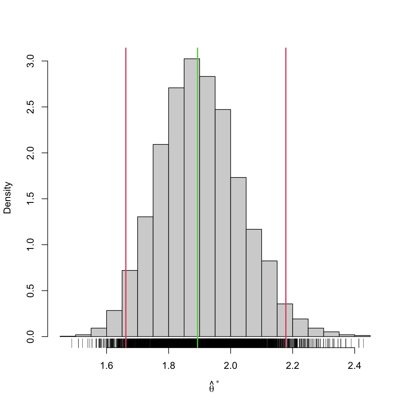

##     2.5%    97.5% 
## 1.662018 2.178031

We can compare this confidence interval with that given asymptotically in Example 5.11:

# Asymptotic confidence interval
alpha <- 0.05
z <- qnorm(alpha / 2, lower.tail = FALSE)
lambda_mle <- 1 / mean(x)
lambda_mle + c(-1, 1) * z * lambda_mle / sqrt(n)
## [1] 1.630952 2.155753

Observe the similarity between $\widehat{\mathrm{CI}}^*_{1-\alpha}(\lambda)$ and $\mathrm{ACI}_{1-\alpha}(\lambda).$ The bootstrap version has been obtained without using the maximum likelihood theory. It is therefore more general, as it only needs to evaluate $\hat{\lambda}$ many times. For that reason, it is also much slower to compute than the asymptotic confidence interval, which in turn requires knowing or being able to compute $\mathcal{I}(\lambda).$

Example 5.13 The bootstrap confidence interval for the gunpowder data in Example 5.2 is also very similar to the normal confidence interval for the mean obtained there:

# Sample
X <- c(916, 892, 895, 904, 913, 916, 895, 885)

# Bootstrap confidence interval
boot_ci(x = X, B = 5e3, theta_hat = mean)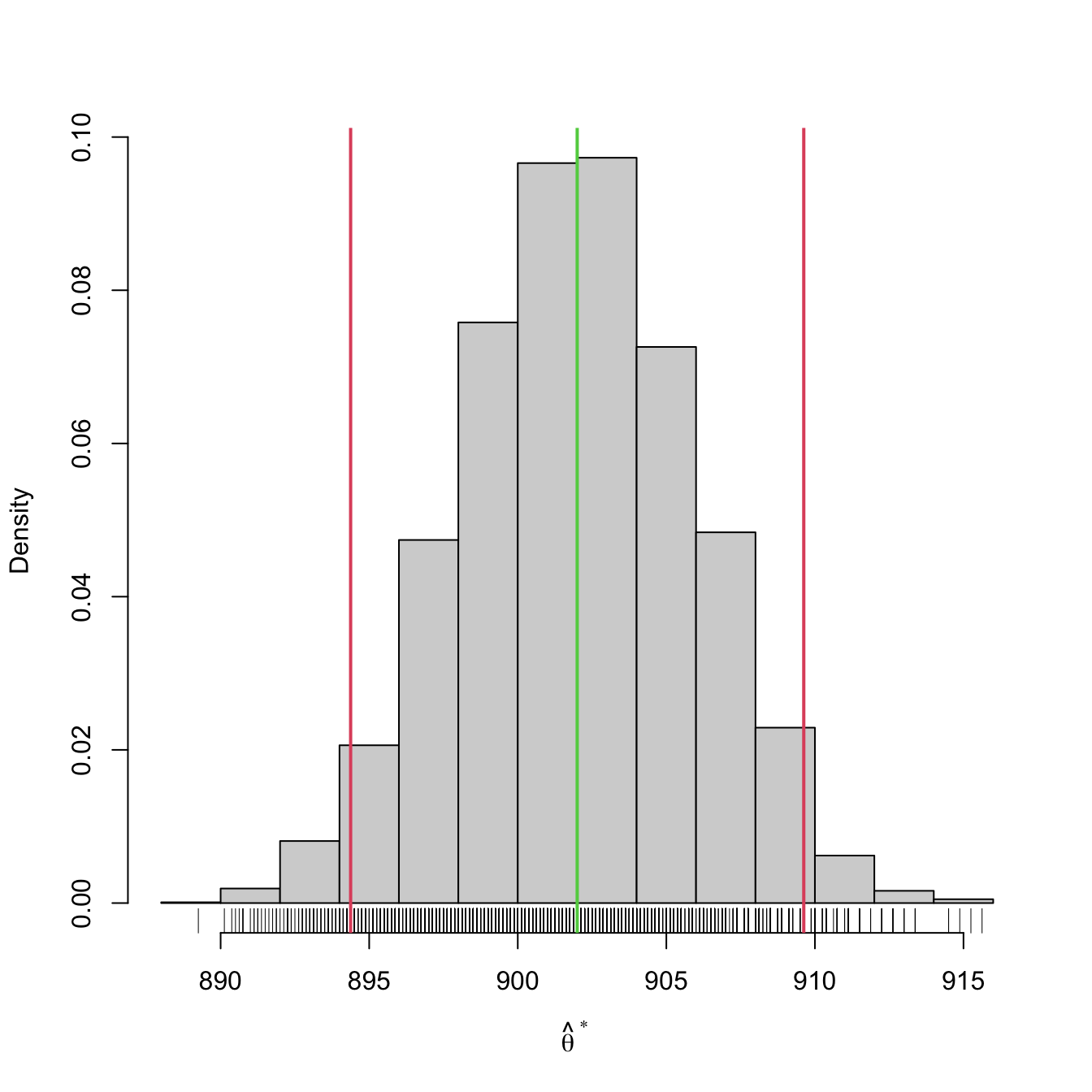

##    2.5%   97.5% 
## 894.375 909.625

Exercises

Exercise 5.1 The daily water consumption in the homes of a specific population can be assumed normally distributed with $\sigma = 16.8$ liters. After an intense campaign to reduce the water consumption, we want to estimate the average daily consumption per home at that population.

What sample size is required to obtain a $\mathrm{CI}_{0.95}(\mu)$ with $2$ liters of error margin?
If the value of $\sigma$ increases, would the needed sample size be bigger or smaller than that required in part a?
If the significance level is $\alpha=0.10,$ would the needed sample size be bigger or smaller than that required in part a?

Exercise 5.2 During the quality control process carried out in a mobile phone company, it turned out that $6$ out of $120$ mobiles randomly selected were defective. Obtain a $99\%$ confidence interval for the proportion of defective mobiles in the manufacturing process of this company.

Exercise 5.3 Assume a sample of size $n=1$ of a $\mathcal{U}(0,\theta)$ distribution, where $\theta$ is unknown. Find the inferior limit of a confidence interval at $0.95$ confidence level for $\theta.$

Exercise 5.4 With the aim of assigning research grants to master students in scientific masters, the Spanish Ministry of Education is analyzing the final grades of students in the scientific BSc’s of the last academic course.

Assuming that the final grades follow approximately a normal distribution. Compute the confidence interval for the mean of the final grades if the following srs of $15$ students is available: $6.2,$ $7.3,$ $5.5,$ $6.7,$ $9.0,$ $7.1,$ $5.0,$ $6.3,$ $7.2,$ $7.5,$ $8.0,$ $7.9,$ $6.5,$ $6.1,$ $7.0.$
Compute the confidence interval for the variance of the final grades.
Compute the confidence interval for the mean if the distribution of final grades is unknown and a srs of $50$ students with $\bar{X}=6.5$ and $S'=1.3$ is available.

Exercise 5.5 In order to estimate the variance of the amount of study hours of the students in a master in statistics, a srs of $20$ students is analysed, resulting in a quasistandard deviation of $2.5$ hours. Determine a confidence interval for the variance at the confidence level $0.90,$ assuming that the weekly study hours follow a normal distribution.

Exercise 5.6 The monthly gross salary of a certain group of professionals roughly follows a log-normal distribution (Exercise 5.19). A union gathers the following srs of salaries, measured in euros:

\[\begin{align*} 2072, 2726, 2254, 3029, 2283, 2673, 2401, 2463, 2416, 2909,\\ 2385, 2055, 2139, 2553, 2453, 2621, 2808, 3583, 2662, 2732,\\ 1996, 2164, 2036, 2915, 2507, 3245, 2337, 2672, 3089, 3012,\\ 2725, 2467, 2439, 2692, 1793, 3845, 2523, 2585, 1647, 2072,\\ 1988, 2767, 3679, 2280, 2642, 3112, 2512, 2435, 2820, 2142,\\ 3197, 3103, 2130, 3213, 2464, 2243, 2958, 2529, 2160, 2484. \end{align*}\]

The union is interested in reporting the $95\%$-confidence interval for the mean to inform its members about the average gross salary in the sector.

Exercise 5.7 The management of a medical clinic wants to estimate the average number of days required for the treatment of the patients with ages between $25$ and $34$ years. A srs of $500$ patients of the clinic with these ages provided $\bar{X}=5.4$ and $S'=3.1$ days. Obtain a confidence interval at confidence level $0.95$ for the mean stay time of the patients.

Exercise 5.8 A poll was made in the fall of 1979 by the Presidential Commission about the retirement policy in the USA. The poll revealed that a large proportion of citizens was very pessimistic about their retirement prospects. When interviewed if they believed that their retirement pension was going to be sufficient, $62.9\%$ of the $6100$ interviewed citizens answered negatively. Compute a $95\%$-confidence interval for the proportion of citizens that believed that their pension would not be sufficient.

Exercise 5.9 Derive a confidence interval for $\sigma,$ the standard deviation of a normal population, based on the derivation of Section 5.2.3.

Exercise 5.10 Consider $X_1,\ldots,X_n\sim \mathcal{N}(\mu,\sigma^2)$ with known $\sigma^2.$ Are you able to derive the following confidence intervals?

$\mathrm{CI}_{1-\alpha}(e^{\mu}).$
$\mathrm{CI}_{1-\alpha}(a\mu+b).$
$\mathrm{CI}_{1-\alpha}(\mu^3).$
$\mathrm{CI}_{1-\alpha}(\mu^2).$
$\mathrm{CI}_{1-\alpha}(\sin(\mu)).$

Reflect on your results.

Exercise 5.11 Replicate Figure 5.1 by coding in R the simulation study behind it.

Exercise 5.12 The oxygen consumption rate is a measure of the physiological activity of runners. Two groups of runners have been trained by two methods: one based on continuous training during a certain period of time each day, and another based on intermittent training with the same duration. Samples were taken from the oxygen consumption of the runners trained by both methods, obtaining the following descriptive statistics:

Continuous training	Intermittent training
$n_1=9$	$n_2=7$
$\bar{X}_1=43.71$	$\bar{X}_2=39.63$
$S_1'^2=5.88$	$S_2'^2=7.68$

It is assumed that the measurements come from independent normal populations with equal variance. Compute the confidence interval of the difference of oxygen consumption rates with a confidence level of $0.95.$

Exercise 5.13 We want to compare the amount of weekly study hours of the students graduated from a BSc in Statistics and a BSc in Economy. For that, we obtained a srs of $20$ students graduated from the BSc in Statistics, with $\bar{X}_1=3$ and $S_1'=2.5,$ and another srs of $30$ students graduated from the BSc in Economy, with $\bar{X}_2=2.8$ and $S_2'=2.7.$ Assume that the weekly study hours follow a normal distribution.

Compute a $95\%$-confidence interval for the ratio of variances of the weekly study hours for both types of students.
Assuming that the variances are equal, obtain a $95\%$-confidence interval for the difference of means of weekly study hours of the two types of students.

Exercise 5.14 Consider $(X_{11},\ldots,X_{1n_1})$ and $(X_{21},\ldots,X_{2n_2})$ two independent srs of rv’s with $\mathcal{N}(\mu_1,\sigma_1^2)$ and $\mathcal{N}(\mu_2,\sigma_2^2)$ distributions, respectively. Prove or disprove that:

$\bar{X}_1-\bar{X}_2$ and $S^2_1/S^2_2$ are independent.
$\bar{X}_1/\bar{X}_2$ and $S^2_2/S^2_1$ are independent.
$\bar{X}_1-\bar{X}_2$ and $\bar{X}_1+\bar{X}_2$ are independent.
$S^2_1/S^2_2$ and $S^2_1S^2_2$ are independent.

Disprove the statements using simulations in R. Prove using mathematical reasoning.

Exercise 5.15 Assume that the final grades of Exercise 5.4 are distributed as $\Gamma(k,\beta)$ with shape $k>0$ (known) and scale $\beta>0$ (unknown).

Find the MLE of $\beta$ and obtain its asymptotic distribution.
From the obtained asymptotic distribution, find a pivot and construct an asymptotic confidence interval for $\beta.$
Estimate the mean final grade and obtain an asymptotic confidence interval at significance level $\alpha=0.05$ by using the results in parts a and b.
Compute the asymptotic confidence interval obtained in part c if we take a srs of $50$ students with $\bar{X}=6.5$ and $S'=1.3.$ Compare the result with the one obtained in part b of Exercise 5.4. Assume $k=50.$

Exercise 5.16 Use R to validate by simulations the claimed coverage $1-\alpha$ of the confidence interval for:

$\mu$ given in Section 5.2.1.
$\mu$ given in Section 5.2.2.
$\sigma^2$ given in Section 5.2.3.

In order to accomplish the exercise efficiently, create a suitable R function that computes the confidence interval and checks if the parameter belongs to it. Then, approximate the coverage probability by the relative frequency of the event “parameter belongs to the confidence interval” using $M=1000$ simulations. You may fix $n=25.$ Set the remaining parameters at your convenience.

Exercise 5.17 The number of needed corrections per page in a book follows a Poisson distribution with parameter $\lambda.$ After proofreading $30$ pages at random, an editor annotates the following amount of required corrections: 1, 2, 2, 1, 0, 1, 0, 0, 1, 1, 0, 0, 1, 1, 2, 0, 1, 1, 2, 1, 0, 0, 0, 0, 2, 0, 2, 0, 0, 1. Compute a $99\%$-confidence interval for $\lambda.$

Exercise 5.18 The pdf of the Rayleigh distribution is given by

\[\begin{align*} f(x;\lambda)=\frac{x}{\lambda^2}e^{-\frac{x^2}{2\lambda^2}},\quad x>0,\ \lambda>0. \end{align*}\]

Given a srs $(X_1,\ldots,X_n)$ from the distribution:

Find $\hat{\lambda}_{\mathrm{MLE}}.$
Derive $\mathcal{I}(\lambda)$ or $\hat{\mathcal{I}}(\lambda).$
Find a pivot and construct an asymptotic confidence interval for $\lambda.$

Exercise 5.19 The pdf of the log-normal distribution $\mathcal{LN}(\mu,\sigma^2)$ is given by

\[\begin{align*} f(x;\mu,\sigma^2)=\frac{1}{x\sqrt{2\pi}\sigma}e^{-\frac{(\log x-\mu)^2}{2\sigma^2}},\quad x>0,\,\mu\in\mathbb{R},\,\sigma>0. \end{align*}\]

Given a srs $(X_1,\ldots,X_n)$ from the distribution:

Find $(\hat{\mu}_{\mathrm{MLE}},\hat{\sigma}^2_{\mathrm{MLE}}).$
Derive $\mathcal{I}(\mu)$ and $\mathcal{I}(\sigma^2).$
Find pivots and construct asymptotic confidence intervals for $\mu$ and $\sigma^2.$

Exercise 5.20 Use R to validate by simulations the claimed coverage $1-\alpha$ of the asymptotic confidence interval for:

$\lambda$ given in Example 5.9.
$\lambda$ given in Example 5.11.
$p_A-p_B$ given in Example 5.10.

In order to accomplish the exercise efficiently, create a suitable R function that computes the confidence interval and checks if the parameter belongs to it. Then, approximate the coverage probability by the relative frequency of the event “parameter belongs to the asymptotic confidence interval” using $M=1000$ simulations. Use:

$n=n_1=n_2=10$ (non-asymptotic case) and
$n=n_1=n_2=100$ (asymptotic-like case).

Set the remaining parameters to your convenience.

Exercise 5.21 Perform bootstrap confidence intervals using boot_ci() for:

Part b in Exercise 5.4.
Exercise 5.6.

Exercise 5.22 In a referendum of a certain country, a famous news channel forecasted that option A would obtain $53.5\%$ of the votes and option B $46.5\%$ using a poll of $704$ people. However, a political crisis has been revealed in the last days of the campaign, where no further polls are allowed, which has made the voters of option A less prone to vote. At the referendum day, the news channel interviews $167$ voters after they had voted. They obtain that $77$ of them voted for option A and $90$ for option B. While the counting is being done, the news channel wants to advance if there is an expected flip in the outcome of the referendum. They want to be sure before the official results are announced.

Use boot_ci() to compute bootstrap $99\%$-confidence intervals for the percentage of votes for option A:

Before voting day.
At the voting day.

What should the news channel report given the results?

Exercise 5.23 Construct a bootstrap confidence interval based on the moment estimator $\hat{\theta}_\mathrm{MM}$ in a $\mathcal{U}(-\theta,\theta)$ distribution with $\theta>0.$ For that purpose, use boot_ci(). Check with simulations that the coverage probability of the bootstrap interval is close to $1-\alpha.$

Exercise 5.24 The pmf of the negative binomial distribution $\mathrm{NB}(r,p)$ is given by

\[\begin{align*} p(x;r,p)=\binom{x+r-1}{x}p^r(1-p)^x,\quad x=0,1,\ldots,r>0,\, 0<p<1. \end{align*}\]

A negative binomial rv measures the number of failures before observing $r$ successes in a sequence of independent Bernoulli trials with success probability $p.$

Use that $\mathbb{E}[\mathrm{NB}(r,p)]=r(1-p)/p$ and $\mathbb{V}\mathrm{ar}[\mathrm{NB}(r,p)]=r(1-p)/p^2$ to derive the moment estimators $\hat{r}_\mathrm{MM}$ and $\hat{p}_\mathrm{MM}.$ Then, using boot_ci(), construct a bootstrap confidence interval for $r$ and check with simulations that the coverage probability of the bootstrap interval is close to $1-\alpha.$

Exercise 5.25 Perform Exercise 5.20 using bootstrap confidence intervals instead of asymptotic confidence intervals. For that purpose, use the function boot_ci() conveniently in parts a and b, and modify it appropriately for part c.

Therefore, it is key that $Z$ is bijective in $\theta$ to be invertible.↩︎
If the distribution of $\hat{\theta}$ is only known asymptotically, then one can build an asymptotic confidence interval through the pivot method; see Section 5.4.↩︎
See Definition 1.7.↩︎
For fixed sample size! The $n$ does not change. What is repeated is the extraction of new samples.↩︎
Other splittings are possible.↩︎
This makes a lot of sense in normal distributions due to the shape of the $\mathcal{N}(0,1)$ pdf: symmetric and decaying monotonically from $0.$↩︎
The definition for discrete rv’s involve considering the smallest $x_\alpha$ such that $\mathbb{P}(X\geq x_{\alpha})\geq\alpha.$↩︎
This is due to tradition and simplicity. Unlike in the normal or Student’s $t$ cases, splitting $\alpha$ evenly at both tails does not give the shortest interval containing $1-\alpha$ probability. However, the shortest confidence interval with $1-\alpha$ coverage is more convoluted.↩︎
This is a particular case of Proposition 1.11.↩︎
This reasoning is not fully rigorous. Using confidence intervals in a chained way may result in a confidence level that is not the nominal one. A more rigorous approach is possible with a confidence interval for $\mu_1-\mu_2$ with $\sigma_1^2\neq\sigma_2^2$ unknown, but it is beyond the scope of this course.↩︎
This step can be excluded if only the confidence interval for $\hat{\theta}$ is desired, as $\mathrm{CI}^*_{1-\alpha}(\theta)$ does not depend on $\hat{\theta}(x_1,\ldots,x_n)$ directly! Nevertheless, it is often useful to know $\hat{\theta}(x_1,\ldots,x_n)$ in addition to the confidence interval.↩︎
What we do in this step is a Monte Carlo simulation of $\hat{\theta}^*$ to approximate the sampling distribution of $\hat{\theta}^*$ with the sample $(\hat{\theta}_1^*,\ldots,\hat{\theta}_B^*).$ In that way, we can approximate $\mathrm{CI}^*_{1-\alpha}(\theta)$ up to arbitrary precision for a large $B.$ This precision is quantified through the standard deviation of the Monte Carlo estimate, which is $C/\sqrt{B}$ with $C>0$ a fixed constant depending on the problem.↩︎
Replacement, i.e., allowing repetitions of elements in $(X_{1,b}^*,\ldots,X_{n,b}^*),$ is key to generate variability.↩︎
Extracting a sample with replacement from another sample is easy in R: if x is the vector containing $(x_1,\ldots,x_n),$ then sample(x, replace = TRUE) draws a sample $(X_{1,b}^*,\ldots,X_{n,b}^*).$↩︎

4 Estimation methods

6 Hypothesis tests

Statistic	Method 1	Method 2
\(n_i\)	\(11\)	\(14\)
\(\bar{X}_i\)	\(64\)	\(69\)
\(S_i'^2\)	\(52\)	\(71\)

Continuous training	Intermittent training
\(n_1=9\)	\(n_2=7\)
\(\bar{X}_1=43.71\)	\(\bar{X}_2=39.63\)
\(S_1'^2=5.88\)	\(S_2'^2=7.68\)

Procedure	Measurements
Standard	\(32 \qquad 37 \qquad 35 \qquad 28 \qquad 41 \qquad 44 \qquad 35 \qquad 31 \qquad 34\)
New	\(35 \qquad 31 \qquad 29 \qquad 25 \qquad 34 \qquad 40 \qquad 27 \qquad 32 \qquad 31\)