4 Estimation methods

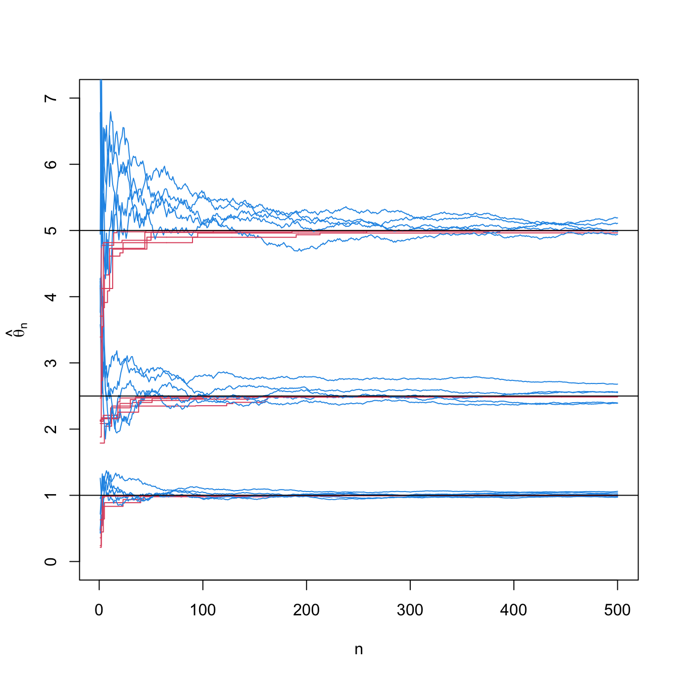
$Convergence of the moment estimator $\hat{\theta}_\mathrm{MM}$ (blue) and maximum likelihood estimator $\hat{\theta}_\mathrm{MLE}$ (red) for $\theta$ in a $\mathcal{U}(0,\theta)$ population. For $\theta=1,2.5,5,$ $N=5$ srs’s of sizes increasing until $n=500$ were simulated. The black horizontal lines represent the values of $\theta.$ The maximum likelihood estimator is more efficient than the moment estimator, as evidenced by the faster convergence of the former.$

Figure 4.1: Convergence of the moment estimator $\hat{\theta}_\mathrm{MM}$ (blue) and maximum likelihood estimator $\hat{\theta}_\mathrm{MLE}$ (red) for $\theta$ in a $\mathcal{U}(0,\theta)$ population. For $\theta=1,2.5,5,$ $N=5$ srs’s of sizes increasing until $n=500$ were simulated. The black horizontal lines represent the values of $\theta.$ The maximum likelihood estimator is more efficient than the moment estimator, as evidenced by the faster convergence of the former.

This chapter is devoted to arguably the two most popular approaches in statistical inference for estimating one or more parameters: the method of moments and maximum likelihood.

In this chapter we start embracing the more realistic case of estimating several parameters of the population, as opposed to the uniparameter view we have been mainly following so far.

4.1 Method of moments

Consider a population $X$ whose distribution depends on $K$ unknown parameters $\boldsymbol{\theta}=(\theta_1,\ldots,\theta_K)^\top.$ If they exist, the population moments are, in general, functions of the unknown parameters $\boldsymbol{\theta}.$ That is,

\[\begin{align*} \alpha_r\equiv\alpha_r(\theta_1,\ldots,\theta_K):=\mathbb{E}[X^r], \quad r=1,2,\ldots \end{align*}\]

Given a srs of $X,$ we denote the sample moment of order $r$ by $a_r$ that estimates $\alpha_r$:

\[\begin{align*} a_r:=\bar{X^r}=\frac{1}{n}\sum_{i=1}^n X_i^r, \quad r=1,2,\ldots \end{align*}\]

Note that the sample moments do not depend on $\boldsymbol{\theta}=(\theta_1,\ldots,\theta_K)^\top$ but the population moments do. This is the key fact that the method of moments exploits for finding the values of the parameters $\boldsymbol{\theta}$ that perfectly equate $\alpha_r$ to $a_r$ for as many $r$’s as necessary.⁴² The overall idea can be abstracted as matching population moments with sample moments and solving for $\boldsymbol{\theta}$.

Definition 4.1 (Method of moments) Let $X\sim F_{\boldsymbol{\theta}}$ with $\boldsymbol{\theta}=(\theta_1,\ldots,\theta_K)^\top.$ From a srs of $X,$ the method of moments produces the estimator $\hat{\boldsymbol{\theta}}_{\mathrm{MM}}$ that is the solution to the system of equations

\[\begin{align*} \alpha_r(\theta_1,\ldots,\theta_K)=a_r, \quad r=1,\ldots, R, \end{align*}\]

where $R\geq K$ is the lowest integer such that the system admits a unique solution and $\theta_1,\ldots,\theta_K$ are the variables. The estimator $\hat{\boldsymbol{\theta}}_{\mathrm{MM}}$ is simply referred to as the moment estimator of $\boldsymbol{\theta}.$

Example 4.1 Assume that we have a population with distribution $\mathcal{N}(\mu,\sigma^2)$ and a srs $(X_1,\ldots,X_n)$ from it. In this case, $\boldsymbol{\theta}=(\mu,\sigma^2)^\top.$ Let us compute the moment estimators of $\mu$ and $\sigma^2.$

For estimating two parameters, we need at least a system with two equations. We compute in the first place the first two moments of the rv $X\sim \mathcal{N}(\mu,\sigma^2).$ The first one is $\alpha_1(\mu,\sigma^2)=\mathbb{E}[X]=\mu.$ The second order moment arises from the variance $\sigma^2$:

\[\begin{align*} \alpha_2(\mu,\sigma^2)=\mathbb{E}[X^2]=\mathbb{V}\mathrm{ar}[X]+\mathbb{E}[X]^2=\sigma^2+\mu^2. \end{align*}\]

On the other hand, the first two sample moments are given by

\[\begin{align*} a_1=\bar{X}, \quad a_2=\frac{1}{n}\sum_{i=1}^n X_i^2=\bar{X^2}. \end{align*}\]

Then, the equations to solve in $(\mu,\sigma^2)$ are

\[\begin{align*} \begin{cases} \mu=\bar{X},\\ \sigma^2+\mu^2=\bar{X^2}. \end{cases} \end{align*}\]

The solution for $\mu$ is already in the first equation. Substituting this value in the second equation and solving $\sigma^2,$ we get the estimators

\[\begin{align*} \hat{\mu}_{\mathrm{MM}}=\bar{X},\quad \hat{\sigma}^2_{\mathrm{MM}}=\bar{X^2}-\hat{\mu}_{\mathrm{MM}}^2=\bar{X^2}-\bar{X}^2=S^2. \end{align*}\]

It turns out the sample mean and sample variance are the moment estimators of $(\mu,\sigma^2).$

Example 4.2 Let $(X_1,\ldots,X_n)$ be a srs of a rv $X\sim\mathcal{U}(0,\theta).$ Let us obtain the estimator of $\theta$ by the method of moments.

The first population moment is $\alpha_1(\theta)=\mathbb{E}[X]=\theta/2$ and the first sample moment is $a_1=\bar{X}.$ Equating both and solving for $\theta,$ we readily obtain $\hat{\theta}_{\mathrm{MM}}=2\bar{X}.$

We can observe that the estimator $\hat{\theta}_{\mathrm{MM}}$ of the upper range limit can be actually smaller than $X_{(n)}.$ Or larger than $\theta,$⁴³ even if we do not have any possible information on the sample above $\theta.$ Then, intuitively, the estimator is clearly suboptimal. This observation is just an illustration of a more general fact that shows that the estimators obtained by the method of moments are usually not the most efficient ones.

Example 4.3 Let $(X_1,\ldots,X_n)$ be a srs of a rv $X\sim\mathcal{U}(-\theta,\theta),$ $\theta>0.$ Obtain the moment estimator of $\theta.$

The first population moment is now $\alpha_1(\theta)=\mathbb{E}[X]=0.$ It does not contain any information about $\theta$! Therefore, we need to look into the second population moment, that is $\alpha_2(\theta)=\mathbb{E}[X^2]=\mathbb{V}\mathrm{ar}[X]+\mathbb{E}[X]^2=\mathbb{V}\mathrm{ar}[X]=\theta^2/3.$ With this moment we can now solve $\alpha_2(\theta)=\bar{X^2}$ for $\theta,$ obtaining $\hat{\theta}_{\mathrm{MM}}=\sqrt{3\bar{X^2}}.$

This example illustrates that in certain situations it may be required to consider $R>K$ equations (here, $R=2$ and $K=1$) to compute the moment estimators if some of them are non-informative.

Example 4.4 We know from (2.7) that $\mathbb{E}[\chi^2_\nu]=\nu.$ Therefore, it is immediate that $\hat{\nu}_{\mathrm{MM}}=\bar{X}.$ Figure 4.2 shows a visualization of how the method of moments operates in this case: it “scans” several degrees of freedom $\nu$ until finding that for which $\nu=\bar{X}.$ In this process, the method of moments only uses the information of the sample realization $x_1,\ldots,x_n$ that is summarized in $\bar{X},$ nothing else.⁴⁴

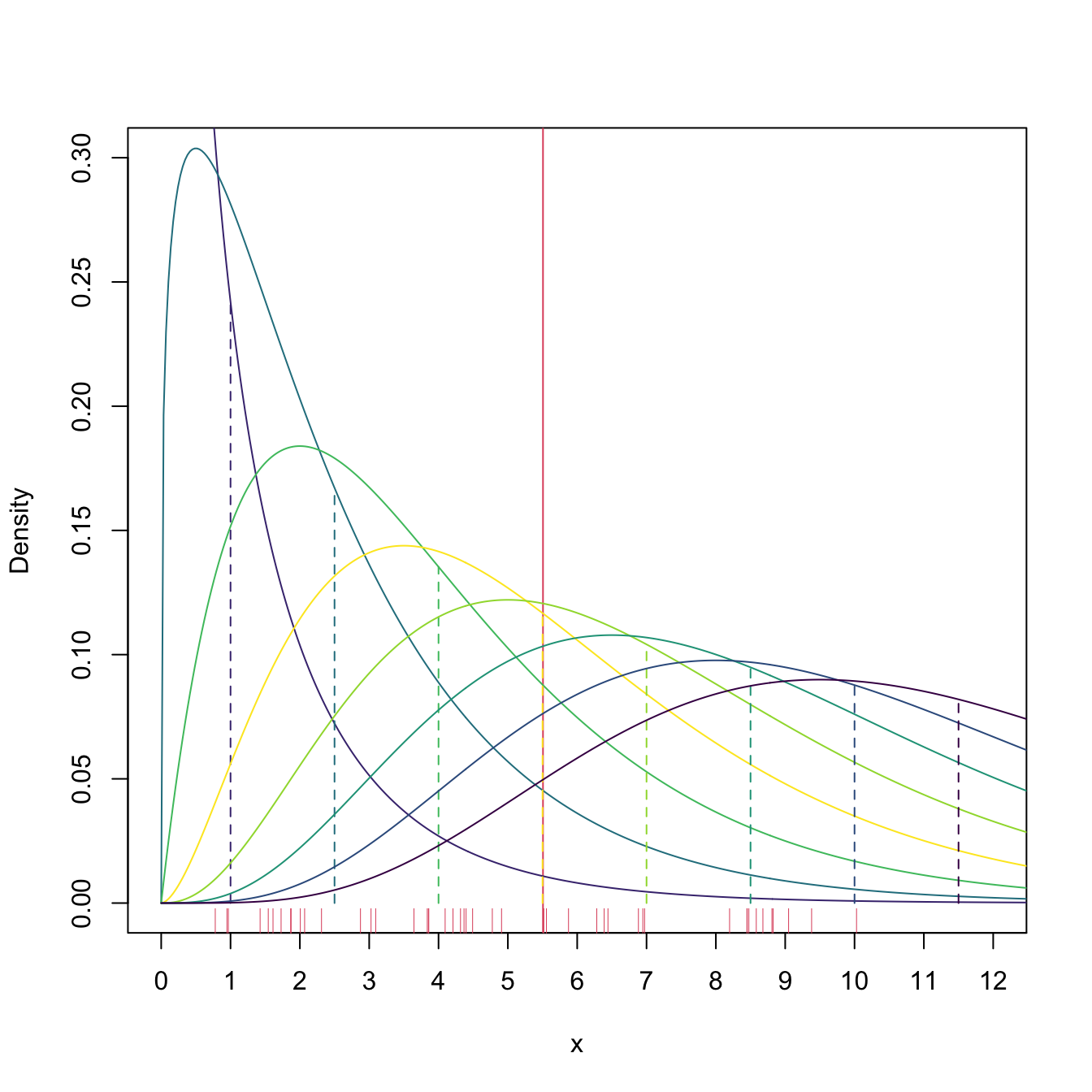
$$\chi^2_\nu$ densities for several degrees of freedom $\nu.$ Their color varies according to how far away the expectation $\nu$ (shown in the vertical dashed lines) is from $\bar{X}\approx5.5$ (red vertical line): the more yellowish, the closer $\nu$ is to $\bar{X}$.$

Figure 4.2: $\chi^2_\nu$ densities for several degrees of freedom $\nu.$ Their color varies according to how far away the expectation $\nu$ (shown in the vertical dashed lines) is from $\bar{X}\approx5.5$ (red vertical line): the more yellowish, the closer $\nu$ is to $\bar{X}$.

An important observation is that, if the parameters to be estimated $\theta_1,\ldots,\theta_K$ can be written as a function of $K$ population moments through continuous functions,

\[\begin{align*} \theta_k=g_k(\alpha_1,\ldots,\alpha_K), \quad k=1,\ldots,K, \end{align*}\]

then the estimator of $\theta_k$ by the method of moments simply follows by replacing $\alpha$’s by $a$’s:

\[\begin{align*} \hat{\theta}_{\mathrm{MM},k}=g_k(a_1,\ldots,a_K). \end{align*}\]

Recall that $g_k$ is such that $\theta_k=g_k\left(\alpha_1(\theta_1,\ldots,\theta_K),\ldots,\alpha_K(\theta_1,\ldots,\theta_K)\right).$ That is, $g_k$ is the $k$-th component of the inverse function of

\[\begin{align*} \alpha:(\theta_1,\ldots,\theta_K)\in\mathbb{R}^K\mapsto \left(\alpha_1(\theta_1,\ldots,\theta_K),\ldots,\alpha_K(\theta_1,\ldots,\theta_K)\right)\in\mathbb{R}^K. \end{align*}\]

Proposition 4.1 (Consistency in probability of the method of moments) Let $(X_1,\ldots,X_n)$ be a srs of a rv $X\sim F_{\boldsymbol{\theta}}$ with $\boldsymbol{\theta}=(\theta_1,\ldots,\theta_K)^\top$ that verifies

\[\begin{align} \mathbb{E}[(X^k-\alpha_k)^2]<\infty, \quad k=1,\ldots,K.\tag{4.1} \end{align}\]

If $\theta_k=g_k(\alpha_1,\ldots,\alpha_K),$ with $g_k$ continuous, then the moment estimator for $\theta_k,$ $\hat{\theta}_{\mathrm{MM},k}=g_k(a_1,\ldots,a_K),$ is consistent in probability:

\[\begin{align*} \hat{\theta}_{\mathrm{MM},k}\stackrel{\mathbb{P}}{\longrightarrow} \theta_k,\quad k=1,\ldots,K. \end{align*}\]

Proof (Proof of Proposition 4.1). Thanks to the condition (4.1), the LLN implies that the sample moments $a_1,\ldots,a_K$ are consistent in probability for estimating the population moments. In addition, the functions $g_k$ are continuous for all $k=1,\ldots,K,$ hence by Theorem 3.3, $\hat{\theta}_k$ is consistent in probability for $\theta_k,$ $k=1,\ldots,K.$

4.2 Maximum likelihood

4.2.1 Maximum likelihood estimator

Maximum likelihood builds on the concept of likelihood already introduced in Definition 3.9.

Example 4.5 Consider an experiment consisting in tossing a coin two times independently. Let $X$ be the rv “number of observed heads in two tosses”. Then, $X\sim \mathrm{Bin}(2,\theta),$ where $\theta=\mathbb{P}(\mathrm{Heads})\in\{0.2,0.8\}.$ That is, the pmf is

\[\begin{align*} p(x;\theta)=\binom{2}{x}\theta^x (1-\theta)^{2-x}, \quad x=0,1,2. \end{align*}\]

Then, the pmf of $X$ according to the possible values of $\theta$ is given in the following table:

$\theta$	$x=0$	$x=1$	$x=2$
$0.20$	$0.64$	$0.32$	$0.04$
$0.80$	$0.04$	$0.32$	$0.64$

At the sight of this table, it seems logical to estimate $\theta$ in the following way: if in the experiment we obtain $x=0$ heads, then we set the estimator $\hat{\theta}=0.2$ since, provided $x=0,$ $\theta=0.2$ is more likely than $\theta=0.8.$ Analogously, if we obtain $x=2$ heads, we set $\hat{\theta}=0.8.$ If $x=1,$ we do not have a clear choice among $\theta=0.2$ and $\theta=0.8,$ since both are equally likely according to the available information, so we can arbitrarily choose one of the values for $\hat{\theta}.$

The previous example illustrates the core idea behind the maximum likelihood method: estimate the unknown parameter $\theta$ with the value that maximizes the probability of obtaining the actually observed sample realization. Or, in other words, to select the most likely value of $\theta$ according to the data at hand. Note, however, that this interpretation is only valid for discrete rv’s $X,$ for which we can define the probability of the sample realization $(X_1=x_1,\ldots,X_n=x_n)$ as $\mathbb{P}(X_1=x_1,\ldots,X_n=x_n;\theta).$ In the continuous case, the probability of a particular sample realization is zero. In this case, it is the $\theta$ that maximizes the density of the sample realization, $f(x_1,\ldots,x_n;\theta),$ the one that delivers the maximum likelihood estimator.

The formal definition of the maximum likelihood estimator is given next.

Definition 4.2 (Maximum likelihood estimator) Let $(X_1,\ldots,X_n)$ be a srs of a rv whose distribution belongs to the family $\mathcal{F}_{\Theta}=\{F(\cdot; \boldsymbol{\theta}): \boldsymbol{\theta}\in\Theta\},$ where $\boldsymbol{\theta}\in\mathbb{R}^K.$ The Maximum Likelihood Estimator (MLE) of $\boldsymbol{\theta}$ is

\[\begin{align*} \hat{\boldsymbol{\theta}}_{\mathrm{MLE}}:=\arg\max_{\boldsymbol{\theta}\in\Theta} \mathcal{L}(\boldsymbol{\theta};X_1,\ldots,X_n). \end{align*}\]

Remark. Quite often, the log-likelihood

\[\begin{align*} \ell(\boldsymbol{\theta};x_1,\ldots,x_n):=\log \mathcal{L}(\boldsymbol{\theta};x_1,\ldots,x_n) \end{align*}\]

is more manageable than the likelihood. As the logarithm function is monotonously increasing, then the maxima of $\ell(\boldsymbol{\theta};x_1,\ldots,x_n)$ and $\mathcal{L}(\boldsymbol{\theta};x_1,\ldots,x_n)$ happen at the same point.

Remark. If the parametric space $\Theta$ is finite, the maximum can be found by exhaustive enumeration of the values $\{\mathcal{L}(\boldsymbol{\theta};x_1,\ldots,x_n):\boldsymbol{\theta}\in\Theta\}$ (as done in Example 4.5).

If the cardinality of $\Theta$ is infinity and $\mathcal{L}(\boldsymbol{\theta};x_1,\ldots,x_n)$ is differentiable with respect to $\theta$ in the interior of $\Theta,$ then we only need to find roots for the so-called log-likelihood equations (usually simpler than the likelihood equations), which characterize the relative extremes of the log-likelihood function:

\[\begin{align*} \frac{\partial}{\partial \boldsymbol{\theta}}\ell(\boldsymbol{\theta};x_1,\ldots,x_n)=\mathbf{0} \iff \frac{\partial}{\partial \theta_k}\ell(\boldsymbol{\theta};x_1,\ldots,x_n)=0, \quad k=1,\ldots,K. \end{align*}\]

The global maximum is found by checking which of the relative extremes is a local maximum and comparing it with the boundary values of $\Theta.$

Remark. The score function is defined as $\boldsymbol{\theta}\in\mathbb{R}^K \mapsto \frac{\partial}{\partial \boldsymbol{\theta}}\log f(x;\boldsymbol{\theta})\in\mathbb{R}^K.$ It plays a relevant role in likelihood theory since it builds the log-likelihood equations to solve:

\[\begin{align*} \frac{\partial}{\partial \boldsymbol{\theta}}\ell(\boldsymbol{\theta};x_1,\ldots,x_n)=\sum_{i=1}^n \frac{\partial}{\partial \boldsymbol{\theta}}\log f(x_i;\boldsymbol{\theta}). \end{align*}\]

Example 4.6 Let $(X_1,\ldots,X_n)$ be a srs of $X\sim\mathcal{N}(\mu,\sigma^2).$ Let us obtain the MLE of $\mu$ and $\sigma^2.$

Since $\boldsymbol{\theta}=(\mu,\sigma^2)^\top,$ the parametric space is $\Theta=\mathbb{R}\times\mathbb{R}_+.$ The likelihood of $\boldsymbol{\theta}$ is given by

\[\begin{align*} \mathcal{L}(\mu,\sigma^2;X_1,\ldots,X_n)=\frac{1}{(\sqrt{2\pi\sigma^2})^n}\exp\left\{-\frac{1}{2\sigma^2}\sum_{i=1}^n(X_i-\mu)^2\right\} \end{align*}\]

and the log-likelihood by

\[\begin{align*} \ell(\mu,\sigma^2;X_1,\ldots,X_n)=-\frac{n}{2}\log(2\pi\sigma^2)-\frac{1}{2\sigma^2}\sum_{i=1}^n(X_i-\mu)^2. \end{align*}\]

The derivatives with respect to $\mu$ and $\sigma^2$ are

\[\begin{align*} \frac{\partial \ell}{\partial \mu} &=\frac{1}{\sigma^2}\sum_{i=1}^n (X_i-\mu)=0,\\ \frac{\partial \ell}{\partial \sigma^2} &= -\frac{n}{2}\frac{1}{\sigma^2}+\frac{\sum_{i=1}^n(X_i-\mu)^2}{2\sigma^4}=0. \end{align*}\]

The solution to the log-likelihood equations is

\[\begin{align*} \hat{\mu}=\bar{X}, \quad \hat{\sigma}^2=\frac{1}{n}\sum_{i=1}^n (X_i-\bar{X})^2=S^2. \end{align*}\]

We can see that the solution is not a minimum,⁴⁵ since taking the limit when $\sigma^2$ approaches zero we obtain

\[\begin{align*} \lim_{\sigma^2 \downarrow 0} \mathcal{L}(\mu,\sigma^2;X_1,\ldots,X_n)=0 <\mathcal{L}(\mu,\sigma^2;X_1,\ldots,X_n), \quad \forall \mu\in\mathbb{R}, \forall \sigma^2>0. \end{align*}\]

In particular,

\[\begin{align*} \lim_{\sigma^2 \downarrow 0} \mathcal{L}(\mu,\sigma^2;X_1,\ldots,X_n)=0 <\mathcal{L}(\hat{\mu},\hat{\sigma}^2;X_1,\ldots,X_n). \end{align*}\]

This means that the solution is not a minimum. If the second derivatives were computed, it could be seen that the Hessian matrix evaluated at $(\hat{\mu},\hat{\sigma}^2)$ is negatively defined, so $\hat{\mu}$ and $\hat{\sigma}^2$ are maximizers of the likelihood. Therefore, $\hat{\mu}_{\mathrm{MLE}}=\bar{X}$ and $\hat{\sigma}^2_{\mathrm{MLE}}=S^2.$

Remark. The normal distribution is the only distribution for which the MLE of its location parameter is the sample mean $\bar{X}.$ Precisely, in the class of pdf’s $\{f(\cdot-\theta):\theta\in\Theta\}$ with differentiable $f,$ if the MLE of $\theta$ is $\hat{\theta}_{\mathrm{MLE}}=\bar{X},$ then $f=\phi.$ This result dates back to Gauss (1809).

The previous example shows that the MLE does not have to be necessarily unbiased, since the sample variance $S^2$ is a biased estimator of the variance $\sigma^2.$

Example 4.7 Consider a continuous parametric space $\Theta=[0,1]$ for the experiment of Example 4.5. Let us obtain the MLE of $\theta.$

In the first place, observe that $\Theta$ is a closed and bounded interval. A continuous function defined on such an interval always has a maximum, that may be in the interval extremes. Therefore, in this situation we must compare the solutions to the log-likelihood with the extremes of the interval.

The likelihood is

\[\begin{align*} \mathcal{L}(\theta;x)=\binom{2}{x}\theta^x(1-\theta)^{2-x}, \quad x=0,1,2. \end{align*}\]

The log-likelihood is then

\[\begin{align*} \ell(\theta;x)=\log\binom{2}{x}+x\log\theta+(2-x)\log(1-\theta), \end{align*}\]

with derivative

\[\begin{align*} \frac{\partial \ell}{\partial \theta}=\frac{x}{\theta}-\frac{2-x}{1-\theta}. \end{align*}\]

Equating to zero this derivative, and assuming that $\theta\neq 0,1$ (boundary of $\Theta,$ where $\ell$ is not differentiable), we obtain the equation

\[\begin{align*} x(1-\theta)-(2-x)\theta=0. \end{align*}\]

Solving for $\theta,$ we obtain

\[\begin{align*} \hat{\theta}=\frac{x}{2}, \end{align*}\]

that is, the proportion of heads obtained in the two tosses. Comparing the likelihood evaluated at $\hat{\theta}$ with the one of the values of $\theta$ at the boundary of $\Theta,$ we have

\[\begin{align*} \mathcal{L}(0;x)=\mathcal{L}(1;x)=0\leq \mathcal{L}(\hat{\theta};x). \end{align*}\]

Therefore, $\hat{\theta}_\mathrm{MLE}=X/2.$⁴⁶

The following example shows a likelihood that is not continuous for all the possible values of $\theta$ but that it delivers the MLE of $\theta.$

Example 4.8 Let $X\sim \mathcal{U}(0,\theta)$ with pdf

\[\begin{align*} f(x;\theta)=\frac{1}{\theta}1_{\{0\leq x\leq \theta\}}, \quad \theta>0, \end{align*}\]

where $\theta$ is unknown, and let $(X_1,\ldots,X_n)$ be a srs of $X.$ Let us compute the MLE of $\theta.$

The likelihood is given by

\[\begin{align*} \mathcal{L}(\theta;X_1,\ldots,X_n)=\frac{1}{\theta^n}, \quad 0\leq X_1,\ldots,X_n\leq \theta. \end{align*}\]

The restriction involving $\theta$ can be included within the likelihood function (which will take otherwise the value $0$), rewriting it as

\[\begin{align*} \mathcal{L}(\theta;X_1,\ldots,X_n)=\frac{1}{\theta^n}1_{\{X_{(1)}\geq0\}}1_{\{X_{(n)}\leq\theta\}}. \end{align*}\]

We can observe that for $\theta>X_{(n)},$ $\mathcal{L}$ decreases when $\theta$ increases, that is, $\mathcal{L}$ is decreasing in $\theta$ for $\theta>X_{(n)}.$ However, for $\theta<X_{(n)},$ the likelihood is zero. Therefore, the maximum is attained precisely at $\hat{\theta}=X_{(n)}$ and, as a consequence, $\hat{\theta}_{\mathrm{MLE}}=X_{(n)}.$ Figure 4.3 helps visualizing this reasoning.

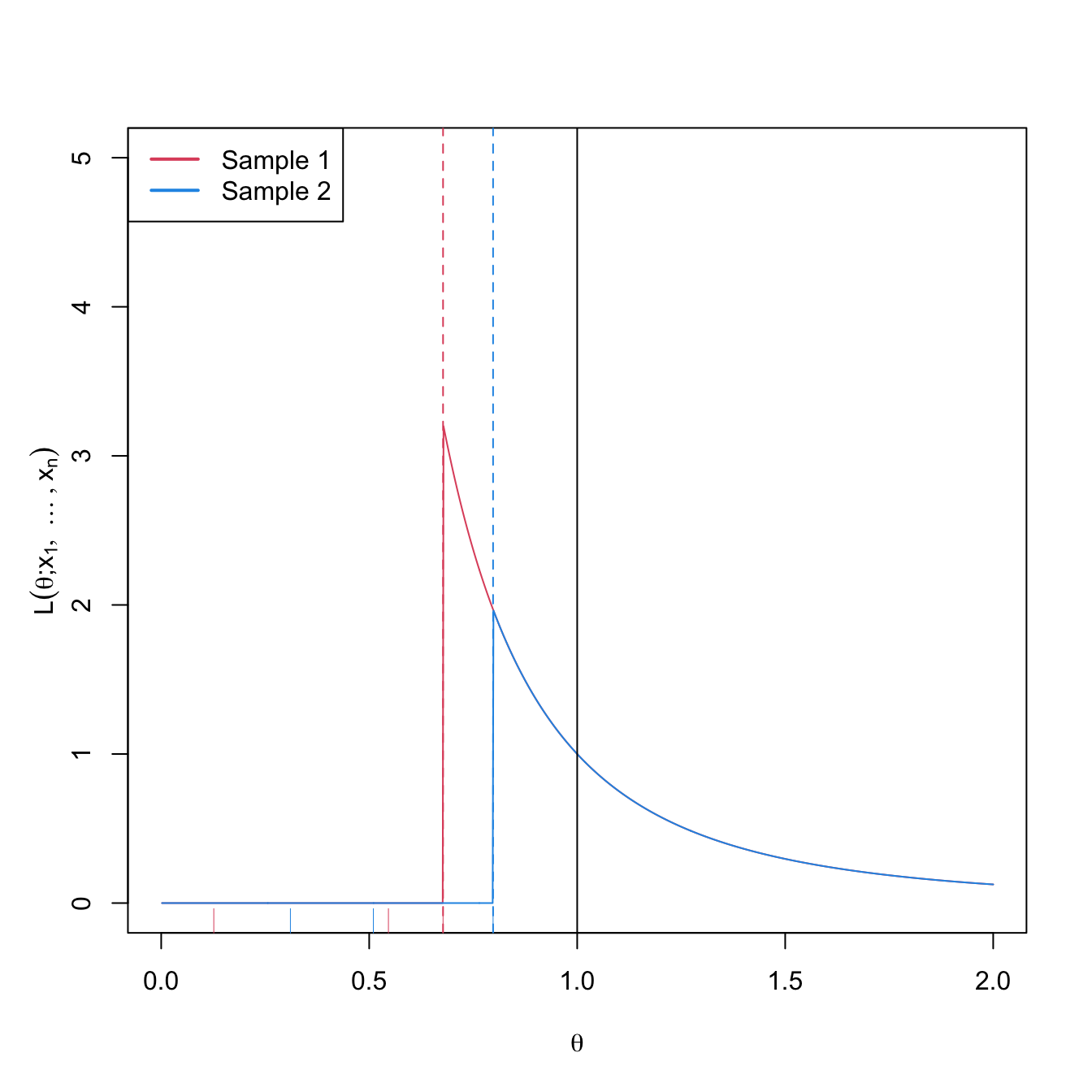
$Likelihood $\mathcal{L}(\theta;x_1,\ldots,x_n)$ as a function of $\theta\in \lbrack0,1\rbrack$ for $\mathcal{U}(0,\theta),$ $\theta=1,$ and two different samples (red and blue) with $n=3.$ The dashed vertical lines represent $\hat{\theta}_{\mathrm{MLE}}=x_{(n)}$ (for the red and blue samples) and $\theta=1$ is shown in black. The ticks on the horizontal axis represent the two samples.$

Figure 4.3: Likelihood $\mathcal{L}(\theta;x_1,\ldots,x_n)$ as a function of $\theta\in \lbrack0,1\rbrack$ for $\mathcal{U}(0,\theta),$ $\theta=1,$ and two different samples (red and blue) with $n=3.$ The dashed vertical lines represent $\hat{\theta}_{\mathrm{MLE}}=x_{(n)}$ (for the red and blue samples) and $\theta=1$ is shown in black. The ticks on the horizontal axis represent the two samples.

The next example shows that the MLE does not have to be unique.

Example 4.9 Let $X\sim \mathcal{U}(\theta-1,\theta+1)$ with pdf

\[\begin{align*} f(x;\theta)=\frac{1}{2}1_{\{x\in[\theta-1,\theta+1]\}}, \end{align*}\]

where $\theta>0$ is unknown, and let $(X_1,\ldots,X_n)$ be a srs of $X.$ Let us compute the MLE of $\theta.$

The likelihood is given by

\[\begin{align*} \mathcal{L}(\theta;X_1,\ldots,X_n)=\frac{1}{2^n}1_{\{X_{(1)}\geq \theta-1\}} 1_{\{X_{(n)}\leq \theta+1\}}=\frac{1}{2^n}1_{\{X_{(n)}-1\leq \theta\leq X_{(1)}+1\}}. \end{align*}\]

Therefore, $\mathcal{L}(\theta;X_1,\ldots,X_n)$ is constant for any value of $\theta$ in the interval $[X_{(n)}-1,X_{(1)}+1],$ and is zero if $\theta$ is not in that interval. This means that any value inside $[X_{(n)}-1,X_{(1)}+1]$ is a maximum and, therefore, a MLE.

The MLE is a function of any sufficient statistic. However, this function does not have to be bijective, and as a consequence, the MLE is not guaranteed to be sufficient (any sufficient statistic can be transformed into the MLE, but the MLE can not be transformed into any sufficient statistic). The next example shows a MLE that is not sufficient.

Example 4.10 Let $X\sim\mathcal{U}(\theta,2\theta)$ with pdf

\[\begin{align*} f(x;\theta)=\frac{1}{\theta}1_{\{\theta\leq x\leq 2\theta\}}, \end{align*}\]

where $\theta>0$ is unknown. Obtain the MLE of $\theta$ from a srs $(X_1,\ldots,X_n).$

The likelihood is

\[\begin{align*} \mathcal{L}(\theta;X_1,\ldots,X_n)=\frac{1}{\theta^n}1_{\{X_{(1)}\geq \theta\}}1_{\{X_{(n)}\leq 2\theta\}}=\frac{1}{\theta^n}1_{\{X_{(n)}/2\leq \theta\leq X_{(1)}\}}. \end{align*}\]

Because of Theorem 3.5, the statistic

\[\begin{align*} T=(X_{(1)},X_{(n)}) \end{align*}\]

is sufficient. On the other hand, since $\mathcal{L}(\theta;X_1,\ldots,X_n)$ is decreasing in $\theta,$ then the maximum is obtained at

\[\begin{align*} \hat{\theta}=\frac{X_{(n)}}{2}, \end{align*}\]

which is not sufficient, since $\mathcal{L}(\theta;X_1,\ldots,X_n)$ can not be factorized adequately.

In addition, the MLE verifies that if there exists an unbiased and efficient estimator for $\theta,$ then this has to be the unique MLE of $\theta.$

Proposition 4.2 (Invariance of the MLE) The MLE is invariant with respect to bijective transformations of the parameter. That is, if $\phi=h(\theta),$ where $h$ is bijective and $\hat{\theta}$ is the MLE of $\theta\in\Theta,$ then $\hat{\phi}=h(\hat{\theta})$ is the MLE of $\phi\in \Phi=h(\Theta).$⁴⁷

Proof (Proof of Proposition 4.2). Let $\mathcal{L}_{\theta}(\theta;X_1,\ldots,X_n)$ be the likelihood of $\theta$ for the srs $(X_1,\ldots,X_n).$ The likelihood of $\phi$ verifies

\[\begin{align*} \mathcal{L}_{\phi}(\phi;X_1,\ldots,X_n)=\mathcal{L}_{\theta}(\theta;X_1,\ldots,X_n)=\mathcal{L}_{\theta}(h^{-1}(\phi);X_1,\ldots,X_n), \quad\forall \phi\in\Phi. \end{align*}\]

If $\hat{\theta}$ is the MLE of $\theta$ then, by definition,

\[\begin{align*} \mathcal{L}_\theta(\hat{\theta};X_1,\ldots,X_n)\geq\mathcal{L}_\theta(\theta;X_1,\ldots,X_n), \quad \forall \theta\in \Theta. \end{align*}\]

Denote $\hat{\phi}=h(\hat{\theta}).$ Since $h$ is bijective, $\hat{\theta}=h^{-1}(\hat{\phi}).$ Then, it follows that

\[\begin{align*} \mathcal{L}_\phi(\hat{\phi};X_1,\ldots,X_n)&=\mathcal{L}_\theta(h^{-1}(\hat{\phi});X_1,\ldots,X_n)=\mathcal{L}_\theta(\hat{\theta};X_1,\ldots,X_n) \\ &\geq \mathcal{L}_\theta(\theta;X_1,\ldots,X_n)=\mathcal{L}_\theta(h^{-1}(\phi);X_1,\ldots,X_n)\\ &=\mathcal{L}_\phi(\phi;X_1,\ldots,X_n), \quad\forall \phi\in\Phi. \end{align*}\]

Therefore, $\hat{\phi}$ is the MLE of $\phi=h(\theta).$

Example 4.11 The lifetime of certain type of light bulbs is a rv $X\sim\mathrm{Exp}(1/\theta).$ After observing the lifetime of $n$ of them, we wish to estimate the probability that the lifetime of a light bulb is above $500$ hours. Let us derive a MLE for this probability.

The pdf of $X$ is

\[\begin{align*} f(x;\theta)=\frac{1}{\theta}e^{-x/\theta}, \quad \theta>0,\ x>0. \end{align*}\]

The probability that a light bulb lasts more than $500$ hours is

\[\begin{align*} \mathbb{P}(X>500)=\int_{500}^{\infty} \frac{1}{\theta}\exp\left\{-\frac{x}{\theta}\right\}\,\mathrm{d}x=\left[-\exp\left\{-\frac{x}{\theta}\right\}\right]_{500}^{\infty}=e^{-500/\theta}. \end{align*}\]

Then, the parameter to estimate is

\[\begin{align*} \phi=e^{-500/\theta}. \end{align*}\]

If we derive $\hat{\theta}_\mathrm{MLE},$ then by Proposition 4.2 we directly obtain $\hat{\phi}_\mathrm{MLE}$ with $\hat{\phi}_\mathrm{MLE}=h(\hat{\theta}_\mathrm{MLE}).$

For the srs $(X_1,\ldots,X_n),$ the likelihood of $\theta$ is

\[\begin{align*} \mathcal{L}(\theta;X_1,\ldots,X_n)=\frac{1}{\theta^n}\exp\left\{-\frac{\sum_{i=1}^n X_i}{\theta}\right\}. \end{align*}\]

The log-likelihood of $\theta$ is

\[\begin{align*} \ell(\theta;X_1,\ldots,X_n)=-n\log\theta-\frac{\sum_{i=1}^n X_i}{\theta}=-n\log\theta-\frac{n\bar{X}}{\theta}. \end{align*}\]

Differentiating and equating to zero,

\[\begin{align*} \frac{\partial \ell}{\partial \theta}=-\frac{n}{\theta}+\frac{n\bar{X}}{\theta^2}=0. \end{align*}\]

Since $\theta\neq 0,$ then solving for $\theta,$ we get

\[\begin{align*} \hat{\theta}=\bar{X}. \end{align*}\]

The second log-likelihood derivative is

\[\begin{align*} \frac{\partial^2\ell}{\partial \theta^2}=\frac{n}{\theta^2}-\frac{2n\bar{X}}{\theta^3}=\frac{1}{\theta^2}\left(n-\frac{2n\bar{X}}{\theta}\right). \end{align*}\]

If we evaluate the second derivative at $\bar{X},$ we get

\[\begin{align*} \left.\frac{\partial^2 \ell}{\partial \theta^2}\right|_{\theta=\bar{X}}=\frac{1}{\bar{X}^2}\left(n-\frac{2n\bar{X}}{\bar{X}}\right)=-\frac{n}{\bar{X}^2}<0,\quad \forall n>0. \end{align*}\]

Therefore, $\hat{\theta}=\bar{X}$ is a local maximum. Since $\Theta=\mathbb{R}_+$ is open and $\hat{\theta}$ is the unique local maximum, then it is a global maximum and hence $\hat{\theta}_\mathrm{MLE}=\bar{X}.$ Therefore, $\hat{\phi}_\mathrm{MLE}=e^{-500/\bar{X}}.$

4.2.2 Asymptotic properties

4.2.2.1 Uniparameter case

One of the most important properties of the MLE is that its asymptotic distribution is completely specified, no matter what is the underlying parametric model as long as it is “regular enough”. The following theorem states the result for the case in which there is only one parameter that is estimated.

Theorem 4.1 (Asymptotic distribution of the MLE; uniparameter case) Let $X\sim f(\cdot;\theta)$ be a continuous rv⁴⁸ whose distribution depends on an unknown single parameter $\theta\in\Theta\subset\mathbb{R}.$ Under certain regularity conditions, any sequence $\hat{\theta}_n$ of roots for the likelihood equation such that $\hat{\theta}_n\stackrel{\mathbb{P}}{\longrightarrow}\theta$ verifies that

\[\begin{align*} \sqrt{n}(\hat{\theta}_n-\theta)\stackrel{d}{\longrightarrow}\mathcal{N}(0,\mathcal{I}(\theta)^{-1}). \end{align*}\]

Remark. Theorem 4.1 is stated for a sequence of roots $\hat{\theta}_n$ such that $\partial \ell(\hat{\theta}_n;X_1,\ldots,X_n)/\partial\theta=0$, i.e., local extrema of the log-likelihood function. These roots are not necessarily the same as the sequence of global maximizers $\hat{\theta}_\mathrm{MLE}$, although in practice they are often the same, at least asymptotically. The reason why asymptotic results for MLE are often stated for sequences of roots $\hat{\theta}_n$ instead of $\hat{\theta}_\mathrm{MLE}$ is technical convenience, and this nuance is often overlooked by regarding $\hat{\theta}_n$ and $\hat{\theta}_\mathrm{MLE}$ as the same object. For simplicity, we will assume this equivalence in the exposition henceforth. See page 123 in Ferguson (1996) for a discussion on this point and counterexamples.

The full list of regularity conditions can be checked in Theorem 2.6 (Section 6.2, page 440) and Theorem 3.10 (Section 6.3, page 449) in Lehmann and Casella (1998). The key points in these assumptions are:

The parameter space $\Theta$ is an open interval of $\mathbb{R}.$
The support of the pdf $f(\cdot;\theta),$ $\mathrm{supp}(f):=\{x\in\mathbb{R}:f(x;\theta)>0\},$ is independent from $\theta.$
$f(\cdot;\theta)$ is three times differentiable and bounded with respect to $\theta\in\Theta$: $\left|\partial^3 f(x;\theta)/\partial\theta^3 \right|\leq M(x),$ for all $x\in \mathrm{supp}(f).$
The Fisher information is such that $0<\mathcal{I}(\theta)<\infty.$

The thesis of Theorem 4.1 can be stated as $\hat{\theta}_\mathrm{MLE}\cong\mathcal{N}(\theta,(n\mathcal{I}(\theta))^{-1}).$ Therefore, the MLE is asymptotically unbiased and asymptotically efficient, in the efficiency sense introduced in Definition 3.13. This means that when the sample size grows, there is no better estimator than the MLE in terms of the MSE. Caveats apply, though, as this is an asymptotic result⁴⁹ that is derived under the above-mentioned regularity conditions.⁵⁰

Corollary 4.1 (Asymptotic unbiasedness and efficiency of the MLE) Under the conditions of Theorem 4.1, the estimator $\hat{\theta}_\mathrm{MLE}$ verifies

\[\begin{align*} \lim_{n\to\infty}\mathbb{E}\big[\hat{\theta}_\mathrm{MLE}\big]=\theta\quad \text{and}\quad \lim_{n\to\infty}\frac{\mathbb{V}\mathrm{ar}\big[\hat{\theta}_\mathrm{MLE}\big]}{(\mathcal{I}_n(\theta))^{-1}}=1. \end{align*}\]

Figure 4.4 gives an insightful visualization of the asymptotic distribution in Theorem 4.1 using Example 4.12.

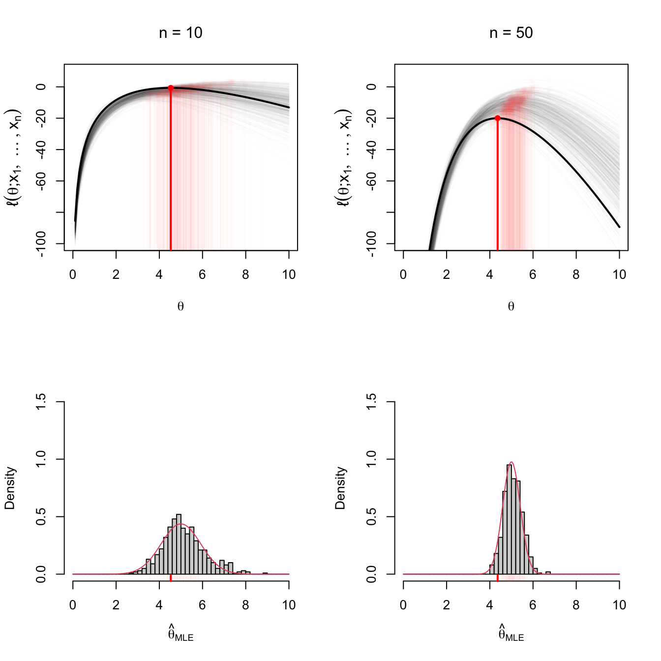
$Visualization of maximum likelihood estimation. The top row shows the (sample-dependent) log-likelihood functions $\theta\mapsto\ell(\theta)$ for $M=500$ samples of sizes $n=10$ (left) and $n=50$ (right). The maximizer of each log-likelihood curve, $\hat{\theta}_{\mathrm{MLE}},$ are shown in red. A particular curve and estimator are highlighted. The bottom row shows histograms of the $M=500$ estimators for $n=10,50$ and the density of $\mathcal{N}(\theta,(n\mathcal{I}(\theta))^{-1}).$ Observe the increment in the curvature of the log-likelihood and the reduction of variance on $\hat{\theta}_{\mathrm{MLE}}$ when $n=10$ and $n=50.$ The model employed in the figure is Example 4.12 with $k=3$ and $\theta=5$.$

Figure 4.4: Visualization of maximum likelihood estimation. The top row shows the (sample-dependent) log-likelihood functions $\theta\mapsto\ell(\theta)$ for $M=500$ samples of sizes $n=10$ (left) and $n=50$ (right). The maximizer of each log-likelihood curve, $\hat{\theta}_{\mathrm{MLE}},$ are shown in red. A particular curve and estimator are highlighted. The bottom row shows histograms of the $M=500$ estimators for $n=10,50$ and the density of $\mathcal{N}(\theta,(n\mathcal{I}(\theta))^{-1}).$ Observe the increment in the curvature of the log-likelihood and the reduction of variance on $\hat{\theta}_{\mathrm{MLE}}$ when $n=10$ and $n=50.$ The model employed in the figure is Example 4.12 with $k=3$ and $\theta=5$.

Example 4.12 Let $(X_1,\ldots,X_n)$ be a srs of the pdf

\[\begin{align} f(x;k,\theta)=\frac{\theta^k}{\Gamma(k)}x^{k-1}e^{-\theta x}, \quad x>0, \ k>0, \ \theta>0, \tag{4.2} \end{align}\]

where $k$ is the shape and $\theta$ is the rate. Note that this is the pdf of a $\Gamma(k,1/\theta)$ as defined in Example 1.21 — the scale $1/\theta$ is the inverse of the rate $\theta.$⁵¹ $\!\!^,$⁵²

We assume $k$ is known and $\theta$ is unknown in this example to compute the MLE of $\theta$ and find its asymptotic distribution.

The likelihood is given by

\[\begin{align*} \mathcal{L}(\theta;X_1,\ldots,X_n)=\frac{\theta^{nk}}{(\Gamma(k))^n}\left(\prod_{i=1}^n X_i\right)^{k-1}e^{-\theta\sum_{i=1}^n X_i}. \end{align*}\]

The log-likelihood is then

\[\begin{align*} \ell(\theta;X_1,\ldots,X_n)=nk\log\theta-n\log\Gamma(k)+(k-1)\sum_{i=1}^n\log X_i-\theta\sum_{i=1}^n X_i. \end{align*}\]

Differentiating with respect to $\theta,$ we get

\[\begin{align*} \frac{\partial \ell}{\partial \theta}=\frac{nk}{\theta}-n\bar{X}=0. \end{align*}\]

Then, the solution of the log-likelihood equation is $\hat{\theta}=k/\bar{X}.$ In addition, $\partial \ell/\partial \theta>0$ if $\theta\in(0,k/\bar{X}),$ while $\partial \ell/\partial \theta<0$ if $\theta\in(k/\bar{X},\infty).$ Therefore, $\ell$ is increasing in $(0,k/\bar{X})$ and decreasing in $(k/\bar{X},\infty),$ which means that it attains the maximum at $k/\bar{X}.$ Therefore, $\hat{\theta}_{\mathrm{MLE}}=k/\bar{X}.$

We compute next the Fisher information of $f(\cdot;\theta).$ For that, we first obtain

\[\begin{align*} \log f(x;\theta)&=k\log\theta-\log\Gamma(k)+(k-1)\log x-\theta x,\\ \frac{\partial \log f(x;\theta)}{\partial \theta}&=\frac{k}{\theta}-x. \end{align*}\]

Squaring and taking expectations, we get⁵³

\[\begin{align} \mathcal{I}(\theta)=\mathbb{E}\left[\left(\frac{\partial \log f(X;\theta)}{\partial \theta}\right)^2\right]=\mathbb{E}\left[\left(\frac{k}{\theta}-X\right)^2\right]=\mathbb{V}\mathrm{ar}[X]=\frac{k}{\theta^2}.\tag{4.3} \end{align}\]

Applying Theorem 4.1, we have that

\[\begin{align*} \sqrt{n}(\hat{\theta}_{\mathrm{MLE}}-\theta)\stackrel{d}{\longrightarrow}\mathcal{N}\left(0,\frac{\theta^2}{k}\right), \end{align*}\]

which means that for large $n,$

\[\begin{align*} \hat{\theta}_{\mathrm{MLE}}\cong \mathcal{N}\left(\theta,\frac{\theta^2}{nk}\right). \end{align*}\]

The visualization in Figure 4.4 serves also to introduce a new optic on the Fisher information $\mathcal{I}(\theta).$ Let us assume that $X\sim f(\cdot;\theta)$ and that $\Theta$ and $f(\cdot;\theta)$ satisfy the full list of regularity conditions above mentioned, which afford the applicability of the Leibniz integral rule.⁵⁴ Then, the expectation of the score function is null:

\[\begin{align*} \mathbb{E}\left[\frac{\partial \log f(X; \theta)}{\partial \theta} \right]=&\;\int_{\mathbb{R}} \frac{\partial \log f(x; \theta)}{\partial \theta} f(x; \theta) \,\mathrm{d} x \\ =&\;\int_{\mathbb{R}} \frac{1}{f(x; \theta)} \frac{\partial f(x; \theta)}{\partial \theta} f(x; \theta) \,\mathrm{d} x \\ =&\;\frac{\partial}{\partial \theta}\int_{\mathbb{R}} f(x; \theta) \,\mathrm{d} x \\ =&\;0. \end{align*}\]

Therefore, the Fisher information $\mathcal{I}(\theta)=\mathbb{E}[(\partial \log f(X; \theta)/\partial \theta)^2]$ is the variance of the score function. Similarly, $\mathbb{E}[\partial \ell(\theta;X_1,\ldots,X_n)/\partial \theta]=0$ and $\mathcal{I}_n(\theta)=\mathbb{V}\mathrm{ar}[\partial \ell(\theta;X_1,\ldots,X_n)/\partial \theta].$ Hence, $\mathcal{I}_n(\theta)$ informs about the expected variability of the relative maximum, $\hat{\theta}_\mathrm{MLE},$ of the log-likelihood: if large, it means that the relative maximum is hard to detect; if small, the relative maximum is well-localized.

Example 4.13 Check that

\[\begin{align} \mathcal{I}(\theta)=-\mathbb{E}\left[\frac{\partial^2 \log f(X; \theta)}{\partial \theta^2}\right].\tag{4.4} \end{align}\]

Expanding the second derivative, we get that

\[\begin{align*} \frac{\partial^2 \log f(x; \theta)}{\partial \theta^2}=&\;\frac{\partial }{\partial \theta}\left[\frac{1}{f(x; \theta)} \frac{\partial f(x; \theta)}{\partial \theta}\right]\\ =&\;-\frac{1}{f(x; \theta)^2}\left(\frac{\partial f(x; \theta)}{\partial \theta}\right)^2+\frac{1}{f(x; \theta)}\frac{\partial^2 f(x; \theta)}{\partial \theta^2}\\ =&\;-\left(\frac{\partial \log f(x; \theta)}{\partial \theta} \right)^2+\frac{1}{f(x; \theta)}\frac{\partial^2 f(x; \theta)}{\partial \theta^2}. \end{align*}\]

The desired equality follows by realizing that the expectation of the first term is zero due to the Leibniz integral rule.

From the equality (4.4), another equivalent view of the Fisher information $\mathcal{I}(\theta)$ is the expected curvature of the log-likelihood function $\theta\mapsto\ell(\theta;X_1,\ldots,X_n)$ at $\theta$ (the true value of the parameter). More precisely, it gives the curvature factor that only depends on the model, since the expected curvature of the log-likelihood function at $\theta$ is $\mathcal{I}_n(\theta)=n\mathcal{I}(\theta).$ Therefore, the larger the Fisher information, the more convex and sharper the log-likelihood function is at $\theta,$ resulting in $\hat{\theta}_\mathrm{MLE}$ being more concentrated about $\theta.$

Example 4.14 From Example 4.13, the Fisher information in (4.3) can be computed as

\[\begin{align*} \mathcal{I}(\theta)=-\mathbb{E}\left[\frac{\partial^2 \log f(X;\theta)}{\partial \theta^2}\right]=-\mathbb{E}\left[-\frac{k}{\theta^2}\right]=\frac{k}{\theta^2}. \end{align*}\]

Analogously, the Fisher information in (3.9) can be computed as

\[\begin{align*} \mathcal{I}(\lambda)=-\mathbb{E}\left[\frac{\partial^2 \log p(X;\lambda)}{\partial \lambda^2}\right]=-\mathbb{E}\left[-\frac{X}{\lambda^2}\right]=\frac{\mathbb{E}[X]}{\lambda^2}=\frac{1}{\lambda}. \end{align*}\]

4.2.2.2 Multiparameter case

The extension of Theorem 4.1 to the multiparameter case in which a vector parameter $\boldsymbol{\theta}\in\Theta\subset\mathbb{R}^K$ is estimated requires the extension of the Fisher information given in Definition 3.12.

Definition 4.3 (Fisher information matrix) Let $X\sim f(\cdot;\boldsymbol{\theta})$ be a continuous rv with $\boldsymbol{\theta}\in\Theta\subset\mathbb{R}^K.$ The Fisher information matrix of $X$ about $\boldsymbol{\theta}$ is defined as⁵⁵

\[\begin{align} \boldsymbol{\mathcal{I}}(\boldsymbol{\theta}):=\mathbb{E}\left[\left(\frac{\partial \log f(x;\boldsymbol{\theta})}{\partial \boldsymbol{\theta}}\right)\left(\frac{\partial \log f(x;\boldsymbol{\theta})}{\partial \boldsymbol{\theta}}\right)^\top\right].\tag{4.5} \end{align}\]

Example 4.15 The Fisher information matrix for a $\mathcal{N}(\mu,\sigma^2)$ is

\[\begin{align*} \boldsymbol{\mathcal{I}}(\mu, \sigma^2)=\begin{pmatrix} 1 / \sigma^2 & 0 \\ 0 & 1 / (2\sigma^4) \end{pmatrix}. \end{align*}\]

Example 4.16 The Fisher information matrix for a $\Gamma(\alpha,\beta)$ (as parametrized in (2.2)) is

\[\begin{align*} \boldsymbol{\mathcal{I}}(\alpha, \beta)=\begin{pmatrix} \psi'(\alpha) & 1 / \beta \\ 1 / \beta & \alpha / \beta^2 \end{pmatrix}, \end{align*}\]

where $\psi(\alpha):=\Gamma'(\alpha) / \Gamma(\alpha)$ is the digamma function.

Example 4.17 The Fisher information matrix for a $\mathrm{Beta}(\alpha,\beta)$ (as parametrized in Exercise 3.19) is

\[\begin{align*} \boldsymbol{\mathcal{I}}(\alpha, \beta)=\begin{pmatrix} \psi'(\alpha)-\psi'(\alpha+\beta) & -\psi'(\alpha+\beta) \\ -\psi'(\alpha+\beta) & \psi'(\beta)-\psi'(\alpha+\beta) \end{pmatrix}. \end{align*}\]

The following theorem is an adaptation of Theorem 5.1 (Section 6.5, page 463) in Lehmann and Casella (1998), where the regularity conditions can be checked. The key points of these conditions are analogous to those in the uniparameter case.

Theorem 4.2 (Asymptotic distribution of the MLE; multiparameter case) Let $X\sim f(\cdot;\boldsymbol{\theta})$ be a continuous rv⁵⁶ whose distribution depends on an unknown vector parameter $\boldsymbol{\theta}\in\Theta\subset\mathbb{R}^K.$ Under certain regularity conditions, with probability tending to $1$ as $n\to\infty,$ there exist roots $\hat{\boldsymbol{\theta}}_n=(\hat{\theta}_{1n},\ldots,\hat{\theta}_{Kn})^\top$ of the likelihood equations such that:

For $k=1,\ldots,K,$ $\hat{\theta}_{kn}\stackrel{\mathbb{P}}{\longrightarrow}\theta_k.$
For $k=1,\ldots,K,$ \[\begin{align} \sqrt{n}(\hat{\theta}_{kn}-\theta_k)\stackrel{d}{\longrightarrow} \mathcal{N}\left(0,[\boldsymbol{\mathcal{I}}(\boldsymbol{\theta})^{-1}]_{kk}\right), \tag{4.6} \end{align}\] where $[\boldsymbol{\mathcal{I}}(\boldsymbol{\theta})^{-1}]_{kk}$ stands for the $(k,k)$-entry of the matrix $\boldsymbol{\mathcal{I}}(\boldsymbol{\theta})^{-1}.$
It also happens that⁵⁷ \[\begin{align} \sqrt{n}(\hat{\boldsymbol{\theta}}_n-\boldsymbol{\theta})\stackrel{d}{\longrightarrow} \mathcal{N}_K\left(\boldsymbol{0},\boldsymbol{\mathcal{I}}(\boldsymbol{\theta})^{-1}\right). \tag{4.7} \end{align}\]

Remark. As in the uniparameter case, under the assumed regularity conditions, the Fisher information matrix (4.5) can be written as

\[\begin{align} \boldsymbol{\mathcal{I}}(\boldsymbol{\theta}):=-\mathbb{E}\left[\frac{\partial^2 \log f(x;\boldsymbol{\theta})}{\partial \boldsymbol{\theta}\partial\boldsymbol{\theta}^\top}\right], \end{align}\]

where $\partial^2 \log f(x;\boldsymbol{\theta})/(\partial \boldsymbol{\theta}\partial\boldsymbol{\theta}^\top)$ is the $K\times K$ Hessian matrix of $\boldsymbol{\theta}\mapsto f(x;\boldsymbol{\theta}).$

Example 4.18 We can apply Theorem 4.2 to the MLE’s of $\boldsymbol{\theta}=(\mu,\sigma^2)^\top$ in a $\mathcal{N}(\mu,\sigma^2)$ rv. From Example 4.6, we know that $\boldsymbol{\hat{\theta}}_{\mathrm{MLE}}=(\bar{X},S^2)^\top.$ Therefore, thanks to Example 4.15, we have that

\[\begin{align*} \sqrt{n}(\boldsymbol{\hat{\theta}}_{\mathrm{MLE}}-\boldsymbol{\theta})=\sqrt{n}\begin{pmatrix}\bar{X}-\mu\\S^2-\sigma^2\end{pmatrix} \stackrel{d}{\longrightarrow}\mathcal{N}_2\left(\begin{pmatrix}0\\0\end{pmatrix},\begin{pmatrix}\sigma^2&0\\0&2\sigma^4\end{pmatrix}\right). \end{align*}\]

This result shows several interesting insights:

It proves that $\bar{X}$ and $S^2$ are asymptotically independent because they are asymptotically joint normal with null covariance. This result is weaker than Fisher’s Theorem (Theorem 2.2), which states that $\bar{X}$ and $S^2$ are independent for any sample size $n.$ But here we are not assuming normality.
It gives that $\sqrt{n}(S^2-\sigma^2)\stackrel{d}{\longrightarrow} \mathcal{N}\left(0,2\sigma^4\right).$ This is equivalent to $\frac{n}{\sigma^2}(S^2-\sigma^2)\cong \mathcal{N}\left(0,2n\right)$ and then to $\frac{nS^2}{\sigma^2}\cong \mathcal{N}\left(n,2n\right).$ Recalling again Fisher’s Theorem, $\frac{nS^2}{\sigma^2}\sim \chi^2_{n-1}.$ Both results are asymptotically equal due to the chi-square approximation (2.15).

We have corroborated that the exact and specific normal theory is indeed coherent with the asymptotic and general maximum likelihood theory.

4.2.2.3 Estimation of the Fisher information matrix

We conclude this section with two important results to turn (4.6) into a more actionable result in statistical inference: (1) replace $\boldsymbol{\mathcal{I}}(\boldsymbol{\theta})$ (unknown if $\boldsymbol{\theta}$ is unknown) with $\boldsymbol{\mathcal{I}}(\hat{\boldsymbol{\theta}}_n)$ (computable); (2) replace $\boldsymbol{\mathcal{I}}(\boldsymbol{\theta})$ (uncomputable in closed form in certain cases, even if $\boldsymbol{\theta}$ is known) with an estimate $\hat{\boldsymbol{\mathcal{I}}}(\boldsymbol{\theta})$ (always computable).

The first result is a direct consequence of the continuous mapping theorem (Theorem 3.3) and the Slutsky Theorem (Theorem 3.4). The result is enough for (uniparameter) inferential purposes on $\theta_k.$

Corollary 4.2 Assume the conditions of Theorem 4.2 holds and that the function $\boldsymbol{\theta}\in\mathbb{R}^K\mapsto\big[\boldsymbol{\mathcal{I}}(\boldsymbol{\theta})^{-1}\big]_{kk}\in\mathbb{R}$ is continuous. Then, for $k=1,\ldots,K,$

\[\begin{align} \frac{\sqrt{n}(\hat{\theta}_{kn}-\theta_k)}{\sqrt{\big[\boldsymbol{\mathcal{I}}(\hat{\boldsymbol{\theta}}_n)^{-1}\big]_{kk}}}\stackrel{d}{\longrightarrow} \mathcal{N}(0,1). \tag{4.8} \end{align}\]

Proof (Proof of Corollary 4.2). Due to the assumed continuity of $\boldsymbol{\theta}\mapsto\big[\boldsymbol{\mathcal{I}}(\boldsymbol{\theta})^{-1}\big]_{kk},$ a generalization of Theorem 3.3 implies that $\big[\boldsymbol{\mathcal{I}}(\hat{\boldsymbol{\theta}}_n)^{-1}\big]_{kk}\stackrel{\mathbb{P}}{\longrightarrow}\big[\boldsymbol{\mathcal{I}}(\boldsymbol{\theta})^{-1}\big]_{kk}$ because of $\hat{\boldsymbol{\theta}}_n\stackrel{\mathbb{P}}{\longrightarrow}\boldsymbol{\theta}$ (which holds, due to Theorem 4.2). Therefore, Theorem 3.4 guarantees that (4.8) is verified.

Remark. Corollary 4.2 can be generalized to the multiparameter case using the Cholesky decomposition⁵⁸ of $\boldsymbol{\mathcal{I}}(\boldsymbol{\theta})=\boldsymbol{R}(\boldsymbol{\theta})\boldsymbol{R}(\boldsymbol{\theta})^\top$ to first turn (4.7) into⁵⁹

\[\begin{align} \sqrt{n}\boldsymbol{R}(\boldsymbol{\theta})^\top(\hat{\boldsymbol{\theta}}_n-\boldsymbol{\theta})\stackrel{d}{\longrightarrow} \mathcal{N}_K\left(\boldsymbol{0},\boldsymbol{I}_K\right) \tag{4.9} \end{align}\]

by using Proposition 1.12. Then,

\[\begin{align*} \sqrt{n}\boldsymbol{R}(\hat{\boldsymbol{\theta}}_n)^\top(\hat{\boldsymbol{\theta}}_n-\boldsymbol{\theta})\stackrel{d}{\longrightarrow} \mathcal{N}_K\left(\boldsymbol{0},\boldsymbol{I}_K\right). \end{align*}\]

Example 4.19 In Example 4.12 we obtained that

\[\begin{align*} \sqrt{n}(\hat{\theta}_{\mathrm{MLE}}-\theta)\stackrel{d}{\longrightarrow}\mathcal{N}\left(0,\frac{\theta^2}{k}\right) \end{align*}\]

or, equivalently, that

\[\begin{align*} \frac{\sqrt{n}(\hat{\theta}_{\mathrm{MLE}}-\theta)}{\theta/\sqrt{k}}\stackrel{d}{\longrightarrow}\mathcal{N}(0,1). \end{align*}\]

In virtue of Corollary 4.2, we can also write

\[\begin{align*} \frac{\sqrt{n}(\hat{\theta}_{\mathrm{MLE}}-\theta)}{\hat{\theta}_{\mathrm{MLE}}/\sqrt{k}}\stackrel{d}{\longrightarrow}\mathcal{N}(0,1). \end{align*}\]

The second result focuses on the form of $\boldsymbol{\mathcal{I}}(\boldsymbol{\theta}).$ As we have seen so far, this Fisher information matrix is not always easy to compute. For example, in Examples 4.16 and 4.17, despite having closed-form solutions, these depend on derivatives of the digamma function. In other cases, the Fisher information matrix does not admit a closed form (see, e.g., Example 4.25). However, as advanced in Exercise 3.25 for the uniparameter case, the Fisher information matrix in (4.5) can be estimated by using its empirical version, in which the expectation is replaced with the sample mean obtained from a srs $(X_1,\ldots,X_n)$ of $X\sim f(\cdot;\boldsymbol{\theta})$:

\[\begin{align} \hat{\boldsymbol{\mathcal{I}}}(\boldsymbol{\theta}):=\frac{1}{n}\sum_{i=1}^n\left(\frac{\partial \log f(X_i;\boldsymbol{\theta})}{\partial \boldsymbol{\theta}}\right)\left(\frac{\partial \log f(X_i;\boldsymbol{\theta})}{\partial \boldsymbol{\theta}}\right)^\top.\tag{4.10} \end{align}\]

The construction is analogous for a discrete rv. The matrix estimator (4.10) is always computable, as no integration is involved, only differentiation.

Due to the LLN (Theorem 3.2), we immediately have that

\[\begin{align*} \hat{\boldsymbol{\mathcal{I}}}(\boldsymbol{\theta})\stackrel{\mathbb{P}}{\longrightarrow}\boldsymbol{\mathcal{I}}(\boldsymbol{\theta}). \end{align*}\]

It can also be shown that, under the conditions of Theorem 4.2,

\[\begin{align*} \hat{\boldsymbol{\mathcal{I}}}(\hat{\boldsymbol{\theta}}_\mathrm{MLE})\stackrel{\mathbb{P}}{\longrightarrow}\boldsymbol{\mathcal{I}}(\boldsymbol{\theta}). \end{align*}\]

This gives the last result of this section, which provides the most usable asymptotic distribution of the MLE.

Corollary 4.3 Assume the conditions of Theorem 4.2 holds, that the function $\boldsymbol{\theta}\in\mathbb{R}^K\mapsto \boldsymbol{\mathcal{I}}(\boldsymbol{\theta})^{-1} \in\mathbb{R}^{K\times K}$ is continuous, and that $\hat{\boldsymbol{\mathcal{I}}}(\boldsymbol{\theta})=\hat{\boldsymbol{R}}(\boldsymbol{\theta})\hat{\boldsymbol{R}}(\boldsymbol{\theta})^\top$ and $\hat{\boldsymbol{\mathcal{I}}}(\hat{\boldsymbol{\theta}}_n)=\hat{\boldsymbol{R}}(\hat{\boldsymbol{\theta}}_n)\hat{\boldsymbol{R}}(\hat{\boldsymbol{\theta}}_n)^\top$ are valid Cholesky decompositions. Then:

$\sqrt{n}\hat{\boldsymbol{R}}(\boldsymbol{\theta})^\top(\hat{\boldsymbol{\theta}}_n-\boldsymbol{\theta})\stackrel{d}{\longrightarrow} \mathcal{N}_K\left(\boldsymbol{0},\boldsymbol{I}_K\right).$
$\sqrt{n}\hat{\boldsymbol{R}}(\hat{\boldsymbol{\theta}}_n)^\top(\hat{\boldsymbol{\theta}}_n-\boldsymbol{\theta})\stackrel{d}{\longrightarrow} \mathcal{N}_K\left(\boldsymbol{0},\boldsymbol{I}_K\right).$

The corollary states that, if challenging or complicated, the Fisher information $\boldsymbol{\mathcal{I}}(\boldsymbol{\theta})$ in the limit distribution of $\sqrt{n}\hat{\boldsymbol{\theta}}_\mathrm{MLE}$ can be replaced with its estimators $\hat{\boldsymbol{\mathcal{I}}}(\boldsymbol{\theta})$ or $\hat{\boldsymbol{\mathcal{I}}}(\hat{\boldsymbol{\theta}}_\mathrm{MLE})$ without altering the asymptotic distribution of $\sqrt{n}\hat{\boldsymbol{\theta}}_\mathrm{MLE}.$

Exercises

Exercise 4.1 The lifetime of a certain type of electrical components follows a $\Gamma(\alpha,\beta)$ distribution, but the values of the parameters $\alpha$ and $\beta$ are unknown. Assume that three of these components are tried in an independent way and the following lifetimes are measured: $120,$ $130,$ and $128$ hours.

Obtain the moment estimators of $\alpha$ and $\beta$ and provide their concrete values for the sample at hand.
Prove the consistency in probability of the estimators by using Corollary 3.3 or Proposition 4.1.

Exercise 4.2 The proportion of impurities in each manufactured unit of a certain kind of chemical product is a rv with pdf

\[\begin{align*} f(x;\theta)=\begin{cases} (\theta+1)x^\theta, & 0<x<1,\\ 0, & \text{otherwise}, \end{cases} \end{align*}\]

where $\theta>-1.$ Five units of the manufactured product are taken in one day, resulting in the next impurity proportions: $0.33,$ $0.51,$ $0.02,$ $0.15,$ $0.12.$

Obtain the moment estimator of $\theta.$
Obtain the maximum likelihood estimator of $\theta.$

Exercise 4.3 An industrial product is packaged in batches of $N$ units each. The number of defective units within each batch is unknown. Since checking whether a unit is defective or not is expensive, the quality control consists in selecting $n$ units of the batch and obtaining an estimation of the number of defective units within the batch. The batch is rejected if the estimated number of defective units exceeds $N/4.$

Find the moment estimator of the number of defective units within a parcel.
If $N=20,$ $n=5,$ and among these $n$ units $2$ of them are defective, is the batch rejected?

Exercise 4.4 Assume that there are $3$ balls in an urn: $\theta$ of them are red and $3-\theta$ white. Two balls are extracted (with replacement).

The two balls are red. Obtain the MLE of $\theta.$
If only one of the balls is red, what is now the MLE of $\theta$?

Exercise 4.5 A particular machine may fail because of two mutually exclusive types of failures: A and B. We wish to estimate the probability of each failure by knowing that:

The probability of failure A is twice the one of B.
In $30$ days we observed $2$ failures of A, $3$ failures of B, and $25$ days without failures.

Compute the moment and maximum likelihood estimators of the probability of each failure.

Exercise 4.6 In the manufacturing process of metallic pieces of three sizes, the proportions of small, normal, and large pieces are $p_1=0.05,$ $p_2=0.9,$ and $p_3=0.05,$ respectively. It is suspected that the machine is not properly adjusted and that the proportions have changed in the following way: $p_1=0.05+\tau,$ $p_2=0.9-2\tau,$ and $p_3=0.05+\tau.$ For checking this suspicion, $5000$ pieces are analyzed, finding $278,$ $4428,$ and $294$ pieces of small, normal, and large sizes, respectively. Compute the MLE of $\tau.$

Exercise 4.7 Let $X_i\sim \mathcal{N}(i\theta, 1),$ $i=1,\ldots,n,$ be independent rv’s.

Obtain the MLE of $\theta.$
Is it unbiased?
Obtain its asymptotic variance.

Exercise 4.8 For $\theta>0,$ let $X$ be a rv with pdf

\[\begin{align*} f(x;\theta)=\frac{\theta}{x^2},\quad x\geq \theta >0. \end{align*}\]

Find the MLE of $\theta.$
Try to obtain the moment estimator of $\theta.$ Is there any problem?

Exercise 4.9 Consider the rv $X$ with pdf

\[\begin{align*} f(x)=\begin{cases} \frac{3\theta^3}{x^4} & \text{if} \ x\geq \theta, \\ 0 & \text{if} \ x< \theta. \end{cases} \end{align*}\]

Find the MLE of $\theta.$
Find the moment estimator $\hat{\theta}_{\mathrm{MM}}.$ Does it always make sense?
Is $\hat{\theta}_{\mathrm{MM}}$ unbiased?
Compute the precision of $\hat{\theta}_{\mathrm{MM}}.$

Exercise 4.10 A srs of size $n$ from the pdf

\[\begin{align*} f(x)=2\theta xe^{-\theta x^2},\quad x>0, \end{align*}\]

where $\theta>0$ is an unknown parameter, is available.

Determine the moment estimator of $\theta.$
Determine the MLE of $\theta$ and find its asymptotic distribution.

Exercise 4.11 Let $(X_1,\ldots,X_n)$ be a srs from the inverse gamma distribution, whose pdf is

\[\begin{align*} f(x;\alpha,\beta)=\frac{\beta^\alpha}{\Gamma(\alpha)}x^{-(\alpha+1)}e^{-\beta/x}, \quad x>0, \ \alpha>0, \ \beta>0. \end{align*}\]

Obtain $\hat{\beta}_{\mathrm{MM}}$ assuming $\alpha$ is known.
Obtain $\hat{\beta}_{\mathrm{MLE}}$ assuming $\alpha$ is known.
Try to obtain $(\hat{\alpha}_{\mathrm{MM}},\hat{\beta}_{\mathrm{MM}}).$

Exercise 4.12 Let $(X_1,\ldots,X_n)$ be a srs from the inverse Gaussian distribution, whose pdf is

\[\begin{align*} f(x;\mu,\lambda)=\sqrt{\frac{\lambda}{2\pi x^3}}\exp\left\{-\frac{\lambda(x-\mu)^2}{2\mu^2x}\right\}, \quad x>0, \ \mu>0, \ \lambda>0. \end{align*}\]

Estimate $\mu$ and $\lambda$ by:

Maximum likelihood.
The method of moments.

Exercise 4.13 Consider the pdf given by

\[\begin{align*} f(x;\theta) = \frac{\theta^2}{1+\theta}(1+x)e^{-\theta x}, \quad x>0,\ \theta>0, \end{align*}\]

and assume a srs $(X_1,\ldots,X_n)$ from it is given.

Obtain $\hat{\theta}_\mathrm{MLE}.$
Obtain the asymptotic variance of $\hat{\theta}_\mathrm{MLE}.$

Exercise 4.14 Consider the following mixture of normal pdf’s:

\[\begin{align} f(x;\boldsymbol{\theta})=w\phi(x;\mu,\sigma^2)+(1-w)\phi(x;-\mu,\sigma^2),\tag{4.11} \end{align}\]

where $\boldsymbol{\theta}=(\mu,\sigma^2,w)^\top\in\mathbb{R}\times\mathbb{R}_+\times[0,1].$ Assume there is a srs $(X_1,\ldots,X_n)$ from $f(\cdot;\boldsymbol{\theta}).$ Then:

Derive the moment estimators of $\boldsymbol{\theta}.$ You can use that $\mathbb{E}[\mathcal{N}(\mu,\sigma^2)^3]=\mu^3+3 \mu \sigma^2$ and $\mathbb{E}[\mathcal{N}(\mu,\sigma^2)^4]=\mu^4+6 \mu^2 \sigma^2+3 \sigma^4.$
Implement in R the moment estimator to verify its correct behavior using a simulated sample from (4.11).
Try to derive the MLE of $\boldsymbol{\theta}.$ Is it simpler or harder than deriving the moment estimators?

Exercise 4.15 Derive the Fisher information matrix in Example 4.15.

Exercise 4.16 Derive the Fisher information matrix in Example 4.16.

Exercise 4.17 Consider a srs $(X_1,Y_1),\ldots,(X_n,Y_n)$ from a bivariate random vector distributed as $\mathcal{N}_2\left(\begin{pmatrix}0\\0\end{pmatrix},\begin{pmatrix}1&\rho\\\rho&1\end{pmatrix}\right).$ Find:

The MLE of $\rho$ (at least in an implicit form).
The asymptotic distribution of $\hat{\rho}_\mathrm{MLE}.$

Exercise 4.18 Replicate Figure 4.1 by coding in R the simulation study behind it.

Exercise 4.19 Replicate Figure 4.4 by coding in R the simulation study behind it. Use rgamma(n = n, shape = k, rate = theta) to simulate a srs of size $n$ from a $\Gamma(k,\theta).$

Exercise 4.20 Validate empirically (4.7) in Theorem 4.2 by coding in R a simulation study that delivers a visualization of the MLE’s distribution similar to the lower plots of Figure 4.4, but for the bivariate case. For that, use scatterplots rather than histograms and contourlines of the bivariate standard normal density. Use the $\Gamma(k,\theta)$ distribution (both parameters unknown) with Fisher information matrix given in Example 4.16.

Some help:

Compute numerically $(\hat{\theta}_\mathrm{MLE},\hat{k}_\mathrm{MLE})$ using the functionMASS::fitdistr(..., densfun = "gamma").
The computation of $\psi$ and $\psi'$ (first and second derivatives of $\log\Gamma$) can be done with numDeriv::grad() and numDeriv::hessian().
Draw contours of a bivariate normal using contour() and mvtnorm::dmvnorm().

Exercise 4.21 Perform the analogous experiment to Exercise 4.20 for the $\mathrm{Beta}(\alpha,\beta)$ distribution (both parameters unknown) with Fisher information matrix given in Example 4.17. Additionally, show the contourplots of several (random) log-likelihood functions, as well as their maxima, in the spirit of the upper plots in Figure 4.4.

Exercise 4.22 Given a srs $(X_1,\ldots,X_n)$ from a $\Gamma(\theta,3)$ distribution, let us investigate the precision of the estimation of the Fisher information $\mathcal{I}(\theta)$ using three approximations:

$\mathcal{I}(\hat{\theta}_\mathrm{MLE}).$
$\hat{\mathcal{I}}(\theta).$
$\hat{\mathcal{I}}(\hat{\theta}_\mathrm{MLE}).$

Draw the above estimates as a function of $n$ to have a plot in the spirit of Figure 4.1, but to estimate $\mathcal{I}(\theta).$ Use $\theta=2,5,$ $N=5$ repetitions, and an increasing sequence of $n$’s until $n=300.$ Importantly, use the same sample to compute the estimators in a–c to allow for a better comparison. Which estimator seems to perform better? Which ones are almost equivalent?

Exercise 4.23 Use simulations to empirically validate the following asymptotic distributions of the MLE for the uniparameter case:

$\sqrt{n\mathcal{I}(\theta)}(\hat{\theta}_{\mathrm{MLE}}-\theta)\stackrel{d}{\longrightarrow}\mathcal{N}(0,1).$
$\sqrt{n\hat{\mathcal{I}}(\theta)}(\hat{\theta}_{\mathrm{MLE}}-\theta)\stackrel{d}{\longrightarrow}\mathcal{N}(0,1).$
$\sqrt{n\mathcal{I}(\hat{\theta}_{\mathrm{MLE}})}(\hat{\theta}_{\mathrm{MLE}}-\theta)\stackrel{d}{\longrightarrow}\mathcal{N}(0,1).$
$\sqrt{n\hat{\mathcal{I}}(\hat{\theta}_{\mathrm{MLE}})}(\hat{\theta}_{\mathrm{MLE}}-\theta)\stackrel{d}{\longrightarrow}\mathcal{N}(0,1).$

Consider the $\mathrm{Beta}(\alpha,\theta)$ distribution with $\alpha$ known and $\theta$ unknown, and Fisher information given in Example 4.17. Then, simulate $N=1000$ srs’s of size $n$ from $\mathrm{Beta}(\alpha,\theta)$ and show the histograms for the random variables in a–d, as well as the standard normal density. Set $\alpha,$ $\theta,$ and $n$ to values of your choice.

Exercise 4.24 Use simulations to empirically validate the following asymptotic distributions of the MLE for the multiparameter case:

$\sqrt{n}\boldsymbol{R}(\boldsymbol{\theta})^\top(\hat{\boldsymbol{\theta}}_\mathrm{MLE}-\boldsymbol{\theta})\stackrel{d}{\longrightarrow} \mathcal{N}_2\left(\boldsymbol{0},\boldsymbol{I}_2\right).$
$\sqrt{n}\hat{\boldsymbol{R}}(\boldsymbol{\theta})^\top(\hat{\boldsymbol{\theta}}_\mathrm{MLE}-\boldsymbol{\theta})\stackrel{d}{\longrightarrow} \mathcal{N}_2\left(\boldsymbol{0},\boldsymbol{I}_2\right).$
$\sqrt{n}\boldsymbol{R}(\hat{\boldsymbol{\theta}}_\mathrm{MLE})^\top(\hat{\boldsymbol{\theta}}_\mathrm{MLE}-\boldsymbol{\theta})\stackrel{d}{\longrightarrow} \mathcal{N}_2\left(\boldsymbol{0},\boldsymbol{I}_2\right).$
$\sqrt{n}\hat{\boldsymbol{R}}(\hat{\boldsymbol{\theta}}_\mathrm{MLE})^\top(\hat{\boldsymbol{\theta}}_\mathrm{MLE}-\boldsymbol{\theta})\stackrel{d}{\longrightarrow} \mathcal{N}_2\left(\boldsymbol{0},\boldsymbol{I}_2\right).$

Consider the $\mathrm{Beta}(\alpha,\beta)$ distribution with $\boldsymbol{\theta}=(\alpha,\beta)$ unknown and Fisher information matrix given in Example 4.17. Then, simulate $N=1000$ srs’s of size $n$ from $\mathrm{Beta}(\alpha,\beta)$ and show the scatterplots for the random vectors in a–d, as well as the contourlines of the bivariate standard normal density. Set $\boldsymbol{\theta}$ and $n$ to values of your choice. Use chol() to compute the Cholesky decomposition in R.

Exercise 4.25 The Gumbel distribution $\mathrm{Gumbel}(\mu,\beta)$ has cdf

\[\begin{align*} F(x;\mu,\beta) = e^{-e^{-((x-\mu)/\beta)}}, \quad x\in \mathbb{R} \end{align*}\]

with $\mu \in \mathbb{R}$ and $\beta>0.$ It is used in extreme value theory to model the maximum of a number of samples of various distributions. Let $(X_1,\ldots,X_n)$ be a srs from a $\mathrm{Gumbel}(\mu,\beta)$ distribution.

Obtain the system of equations to compute $\hat{\mu}_\mathrm{MLE}$ and $\hat{\beta}_\mathrm{MLE}.$
Obtain $\hat{\boldsymbol{\mathcal{I}}}(\mu,\beta).$
Derive usable asymptotic distributions for $\hat{\mu}_\mathrm{MLE}$ and $\hat{\beta}_\mathrm{MLE}.$

References

Ferguson, T. S. 1996. A Course in Large Sample Theory. Texts in Statistical Science. Boca Raton: Chapman & Hall/CRC. https://doi.org/10.1201/9781315136288.

Gauss, C. F. 1809. Theoria Motus Corporum Coelestium in Sectionibus Conicis Solem Ambientium. Cambridge University Press. Cambridge: Cambridge Library Collection.

Lehmann, E. L., and G. Casella. 1998. Theory of Point Estimation. Second. Springer Texts in Statistics. New York: Springer-Verlag. https://doi.org/10.1007/b98854.

The principle of equating $\alpha_r$ to $a_r$ rests upon the fact that $a_r\stackrel{\mathbb{P}}{\longrightarrow}\alpha_r$ when $n\to\infty$ (see Corollary 3.2).↩︎
Assume $\theta=1$ and $n=2$ with $(x_1,x_2)=(0.5,0.75).$ Then, $\hat{\theta}_{\mathrm{MM}}=1.25,$ but we never observed a quantity above the maximum observed value in the sample.↩︎
In particular, it does not use the form of the pdf.↩︎
But note this does not prove that $(\hat{\mu},\hat{\sigma}^2)$ is a maximum.↩︎
We put $X$ and not $x$ because an estimator is a function of the srs, not of its realization.↩︎
$h(\Theta):=\{h(\theta):\theta\in\Theta\}.$↩︎
An analogous result can be stated as well for a discrete rv $X\sim p(\cdot;\theta).$ We exclude it for the sake of simplicity.↩︎
There could be an estimator that beats the MLE in terms of MSE for $n\leq 7,$ for example. Counterexamples exist, especially when $\boldsymbol{X}$ and $\boldsymbol{\theta}$ are high-dimensional and the sample size is small; see the James–Stein estimator.↩︎
Counterexamples exist also when the regularity conditions are not met.↩︎
Both the shape-rate and the scale-rate parametrizations of the gamma distribution are prevalent in statistics, and this is often a source of confusion. Therefore, when dealing with gamma variables it is better to state its pdf, either (2.2) or (4.2), to avoid ambiguities.↩︎
In R, dgamma(..., shape = k, rate = theta) and dgamma(..., shape = alpha, scale = beta) to use (2.2) or (4.2).↩︎
Observe that $\mathbb{E}[\Gamma(k,1/\theta)]=k/\theta$ and $\mathbb{V}\mathrm{ar}[\Gamma(k,1/\theta)]=k/\theta^2.$↩︎
Specifically, check assumption (d) on page 441 in Lehmann and Casella (1998).↩︎
Note that $\frac{\partial \log f(x;\boldsymbol{\theta})}{\partial \boldsymbol{\theta}}$ is a column vector.↩︎
Again, an analogous result can be stated as well for a discrete rv $X\sim p(\cdot;\boldsymbol{\theta}).$ We exclude it for the sake of simplicity.↩︎
Remember the definition of a multivariate normal from Example 1.31.↩︎
Because $\boldsymbol{\mathcal{I}}(\boldsymbol{\theta})$ is positive definite under the regularity conditions of Theorem 4.2, it admits a Cholesky decomposition $\boldsymbol{\mathcal{I}}(\boldsymbol{\theta})=\boldsymbol{R}(\boldsymbol{\theta})\boldsymbol{R}(\boldsymbol{\theta})^\top$ with $\boldsymbol{R}(\boldsymbol{\theta})$ a lower triangular matrix with positive diagonal entries.↩︎
Recall that $\boldsymbol{\mathcal{I}}(\boldsymbol{\theta})^{-1}=(\boldsymbol{R}(\boldsymbol{\theta})^{-1})^\top\boldsymbol{R}(\boldsymbol{\theta})^{-1}.$↩︎

3 Point estimation

5 Confidence intervals

\(\theta\)	\(x=0\)	\(x=1\)	\(x=2\)
\(0.20\)	\(0.64\)	\(0.32\)	\(0.04\)
\(0.80\)	\(0.04\)	\(0.32\)	\(0.64\)