3 Point estimation

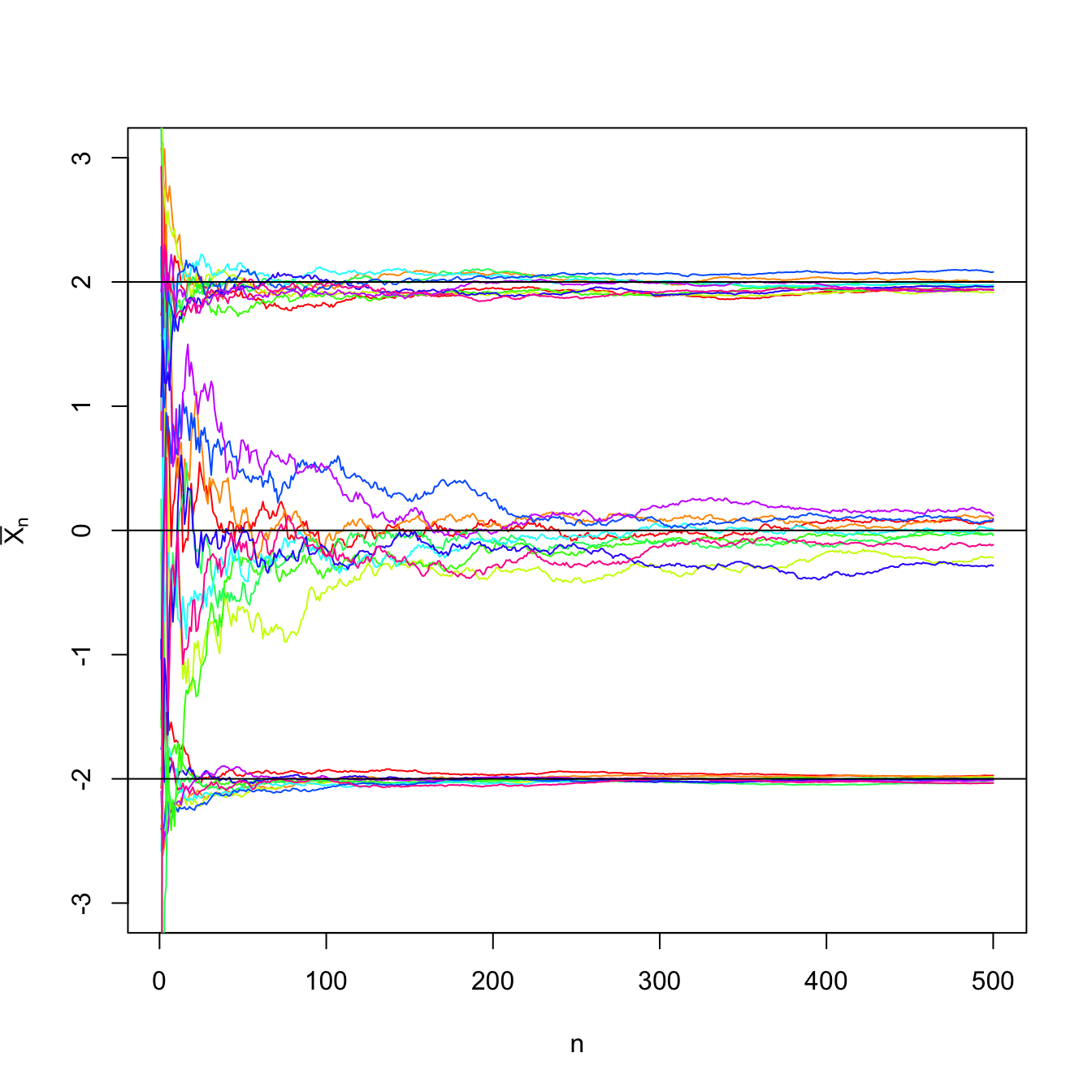
Figure 3.1: Convergence of the sample mean \(\bar{X}_n\) to \(\mu\) in probability as \(n\to\infty\) in a \(\mathcal{N}(\mu,\sigma^2)\) population with \((\mu,\sigma^2)\in\{(-2,0.5),(0,3),(2,1)\}.\) For each set of parameters, \(N=10\) srs’s of sizes increasing until \(n=500\) were simulated. The black horizontal lines represent the values of \(\mu.\) The convergence towards \(\mu\) happens due to the law of large numbers irrespective of the value of \(\sigma^2,\) yet the convergence is faster for smaller variances.

This chapter analyzes the most relevant characteristics of an estimator: bias and mean square error, invariance, consistency, sufficiency, efficiency, robustness, etc.

We begin by introducing the basic terminology.

Definition 3.1 (Estimation, estimator, and estimate) Estimation is the process of inferring or attempting to guess the value of one or several population parameters from a sample. Therefore, an estimator \(\hat{\theta}\equiv\hat{\theta}(X_1,\ldots,X_n)\) of a parameter \(\theta\in\Theta\) is a statistic of the sample \((X_1,\ldots,X_n)\) with range in the parameter space \(\Theta.\) The observed value or realization of an estimator is referred to as estimate.

Example 3.1 The following table shows the usual estimators for well-known parameters.

Parameter	Estimator
Proportion \(p\)	Sample proportion \(\bar{X}\)
Mean \(\mu\)	Sample mean \(\bar{X}\)
Variance \(\sigma^2\)	Sample variance \(S^2\) and quasivariance \(S'^2\)
Standard deviation \(\sigma\)	Sample standard deviation \(S\) and quasistandard deviation \(S'\)

3.1 Unbiased estimators

Definition 3.2 (Unbiased estimator) Given an estimator \(\hat{\theta}\) of a parameter \(\theta,\) the quantity \(\mathrm{Bias}\big[\hat{\theta}\big]:=\mathbb{E}\big[\hat{\theta}\big]-\theta\) is the bias of the estimator \(\hat{\theta}.\) The estimator \(\hat{\theta}\) is unbiased if its bias is zero, i.e., if \(\mathbb{E}\big[\hat{\theta}\big]=\theta.\)

Example 3.2 We saw in (2.5) and (2.6) that the sample variance \(S^2\) was not an unbiased estimator of \(\sigma^2,\) whereas the sample quasivariance \(S'^2\) was unbiased. From Theorem 2.2 we can see, using an alternative approach based on assuming normality, that \(S^2\) is indeed biased. On one hand,

\[\begin{align} \mathbb{E}\left[\frac{nS^2}{\sigma^2}\right]=\mathbb{E}\left[\frac{(n-1)S'^2}{\sigma^2}\right]=\mathbb{E}\left[\chi_{n-1}^2\right]=n-1 \tag{3.1} \end{align}\]

and, on the other,

\[\begin{align} \mathbb{E}\left[\frac{nS^2}{\sigma^2}\right]=\frac{n}{\sigma^2}\mathbb{E}[S^2]. \tag{3.2} \end{align}\]

Therefore, equating (3.1) and (3.2) and solving for \(\mathbb{E}[S^2],\) we have

\[\begin{align*} \mathbb{E}[S^2]=\frac{n-1}{n}\,\sigma^2. \end{align*}\]

We can also see that \(S'^2\) is indeed unbiased. First, we have that

\[\begin{align*} \mathbb{E}\left[\frac{(n-1)S'^2}{\sigma^2}\right]=\frac{n-1}{\sigma^2}\mathbb{E}[S'^2]. \end{align*}\]

Then, equating this expectation with the mean of a rv \(\chi^2_{n-1},\) \(n-1,\) and solving for \(\mathbb{E}[S'^2],\) it follows that \(\mathbb{E}[S'^2]=\sigma^2.\)

Example 3.3 Let \(X\sim\mathcal{U}(0,\theta),\) that is, its pdf is \(f_X(x)=1/\theta,\) \(0<x<\theta.\) Let \((X_1,\ldots,X_n)\) be a srs of \(X.\) Let us obtain an unbiased estimator of \(\theta.\)

Since \(\theta\) is the upper bound for the sample realization, the value from the sample that is closer to \(\theta\) is \(X_{(n)},\) the maximum of the sample. Hence, we take \(\hat{\theta}:=X_{(n)}\) as an estimator of \(\theta\) and check whether it is unbiased. In order to compute its expectation, we need to obtain its pdf. We can derive it from Exercise 2.2: the cdf \(X_{(n)}\) for a srs of a rv with cdf \(F_X\) is \([F_X]^n.\)

The cdf of \(X\) for \(0< x < \theta\) is

\[\begin{align*} F_X(x)=\int_0^x f_X(t)\,\mathrm{d}t=\int_0^x \frac{1}{\theta}\,\mathrm{d}t=\frac{x}{\theta}. \end{align*}\]

Then, the full cdf is

\[\begin{align*} F_X(x)=\begin{cases} 0 & x<0,\\ x/\theta & 0\leq x<\theta,\\ 1 & x\geq \theta. \end{cases} \end{align*}\]

Consequently, the cdf of the maximum is

\[\begin{align*} F_{X_{(n)}}(x)=\begin{cases} 0 & x<0,\\ (x/\theta)^n, & 0\leq x<\theta,\\ 1, & x\geq \theta. \end{cases} \end{align*}\]

The density of \(X_{(n)}\) follows by differentiation:

\[\begin{align*} f_{X_{(n)}}(x)=\frac{n}{\theta}\left(\frac{x}{\theta}\right)^{n-1}, \quad x\in (0,\theta). \end{align*}\]

Finally, the expectation of \(\hat{\theta}=X_{(n)}\) is

\[\begin{align*} \mathbb{E}\big[\hat{\theta}\big]&=\int_0^{\theta} x \frac{n}{\theta}\left(\frac{x}{\theta}\right)^{n-1}\,\mathrm{d}x=\frac{n}{\theta^n}\int_0^{\theta} x^n\,\mathrm{d}x\\ &=\frac{n}{\theta^n}\frac{\theta^{n+1}}{n+1}=\frac{n}{n+1}\theta\neq\theta. \end{align*}\]

Therefore, \(\hat{\theta}\) is not unbiased. However, it can be readily patched as

\[\begin{align*} \hat{\theta}':=\frac{n+1}{n}X_{(n)}, \end{align*}\]

which is an unbiased estimator of \(\theta\):

\[\begin{align*} \mathbb{E}\big[\hat{\theta}'\big]=\frac{n+1}{n}\frac{n}{n+1}\theta=\theta. \end{align*}\]

Example 3.4 Let \(X\sim \mathrm{Exp}(\theta)\) and let \((X_1,\ldots,X_n)\) be a srs of such a rv. Let us find an unbiased estimator for \(\theta.\)

Since \(X\sim \mathrm{Exp}(\theta),\) we know that \(\mathbb{E}[X]=1/\theta\) and hence \(\theta=1/\mathbb{E}[X].\) As \(\bar{X}\) is an unbiased estimator of \(\mathbb{E}[X],\) it is reasonable to consider \(\hat{\theta}:=1/\bar{X}\) as an estimator of \(\theta.\) Checking whether it is unbiased requires knowing the pdf of \(\hat{\theta}.\) Since \(\mathrm{Exp}(\theta)\stackrel{d}{=}\Gamma(1,1/\theta),\) by the additive property of the gamma (see Exercise 1.21):

\[\begin{align*} T=\sum_{i=1}^n X_i\sim \Gamma\left(n,1/\theta\right), \end{align*}\]

with pdf

\[\begin{align*} f_T(t)=\frac{1}{(n-1)!} \theta^n t^{n-1} e^{-\theta t}, \quad t>0. \end{align*}\]

Then, the expectation of the estimator \(\hat{\theta}=n/T=1/\bar{X}\) is given by

\[\begin{align*} \mathbb{E}\big[\hat{\theta}\big]&=\int_0^{\infty} \frac{n}{t}\frac{1}{(n-1)!} \theta^n t^{n-1} e^{-\theta t}\,\mathrm{d}t\\ &=\frac{n \theta}{n-1}\int_0^{\infty}\frac{1}{(n-2)!} \theta^{n-1} t^{(n-1)-1} e^{-\theta t}\,\mathrm{d}t\\ &=\frac{n}{n-1} \theta. \end{align*}\]

Therefore, counterintuitively, \(\hat{\theta}\) is not unbiased for \(\theta.\) However, the corrected estimator

\[\begin{align*} \hat{\theta}'=\frac{n-1}{n}\frac{1}{\bar{X}} \end{align*}\]

is unbiased.

In the previous example we have seen that, even if \(\bar{X}\) is unbiased for \(\mathbb{E}[X],\) \(1/\bar{X}\) is biased for \(1/\mathbb{E}[X].\) This illustrates that, even if \(\hat{\theta}\) is an unbiased estimator of \(\theta,\) then in general a transformation by a function \(g\) results in an estimator \(g(\hat{\theta})\) that is not unbiased for \(g(\theta).\)³²

The quantity \(\hat{\theta}-\theta\) is the estimation error, and depends on the particular value of \(\hat{\theta}\) for the observed (or realized) sample. Observe that the bias is the expected (or mean) estimation error across all possible realizations of the sample, which does not depend on the actual realization of \(\hat{\theta}\) for a particular sample:

\[\begin{align*} \mathrm{Bias}\big[\hat{\theta}\big]=\mathbb{E}\big[\hat{\theta}\big]-\theta=\mathbb{E}\big[\hat{\theta}-\theta\big]. \end{align*}\]

If the estimation error is measured in absolute value, \(|\hat{\theta}-\theta|,\) the quantity \(\mathbb{E}\big[|\hat{\theta}-\theta|\big]\) is referred to as the mean absolute error. If the square is taken, \((\hat{\theta}-\theta)^2,\) then we obtain the so-called Mean Squared Error (MSE)

\[\begin{align*} \mathrm{MSE}\big[\hat{\theta}\big]=\mathbb{E}\big[(\hat{\theta}-\theta)^2\big]. \end{align*}\]

The MSE is mathematically more tractable than the mean absolute error, hence is usually preferred. Since the MSE gives an average of the squared estimation errors, it introduces a performance measure for comparing two estimators \(\hat{\theta}_1\) and \(\hat{\theta}_2\) of a parameter \(\theta.\) The estimator with the lowest MSE is optimal for estimating \(\theta\) according to the MSE performance measure.

A key identity for the MSE is the following bias-variance decomposition:

\[\begin{align*} \mathrm{MSE}\big[\hat{\theta}\big]&=\mathbb{E}\big[(\hat{\theta}-\theta)^2\big]\\ &=\mathbb{E}\big[(\hat{\theta}-\mathbb{E}\big[\hat{\theta}\big]+\mathbb{E}\big[\hat{\theta}\big]-\theta)^2\big]\\ &=\mathbb{E}\big[(\hat{\theta}-\mathbb{E}\big[\hat{\theta}\big])^2\big]+\mathbb{E}\big[(\mathbb{E}[\hat{\theta}]-\theta)^2\big]+2\mathbb{E}\big[(\hat{\theta}-\mathbb{E}\big[\hat{\theta}\big])\big](\mathbb{E}\big[\hat{\theta}\big]-\theta)\\ &=\mathbb{V}\mathrm{ar}\big[\hat{\theta}\big]+(\mathbb{E}[\hat{\theta}]-\theta)^2\\ &=\mathrm{Bias}^2\big[\hat{\theta}\big]+\mathbb{V}\mathrm{ar}\big[\hat{\theta}\big]. \end{align*}\]

This identity tells us that if we want to minimize the MSE, it is not sufficient to find an unbiased estimator: the variance contributes to the MSE the same as the squared bias. Therefore, if we search for the optimal estimator in terms of MSE, both bias and variance must be minimized.

Figure 3.2 shows four extreme cases of the MSE decomposition: (1) low bias and low variance (ideal); (2) low bias and large variance; (3) large bias and low variance; (4) large bias and large variance (worst). The following is a good analogy of these four cases in terms of a game of darts. The bullseye is \(\theta,\) the desired target value to hit. Each dart thrown is a realization of the estimator \(\hat{\theta}.\) The case (1) represents an experienced player: his/her darts land close to the bullseye consistently. Case (2) represents a less skilled player that has high variability about the target. Cases (3) and (4) represent players that make systematic errors.

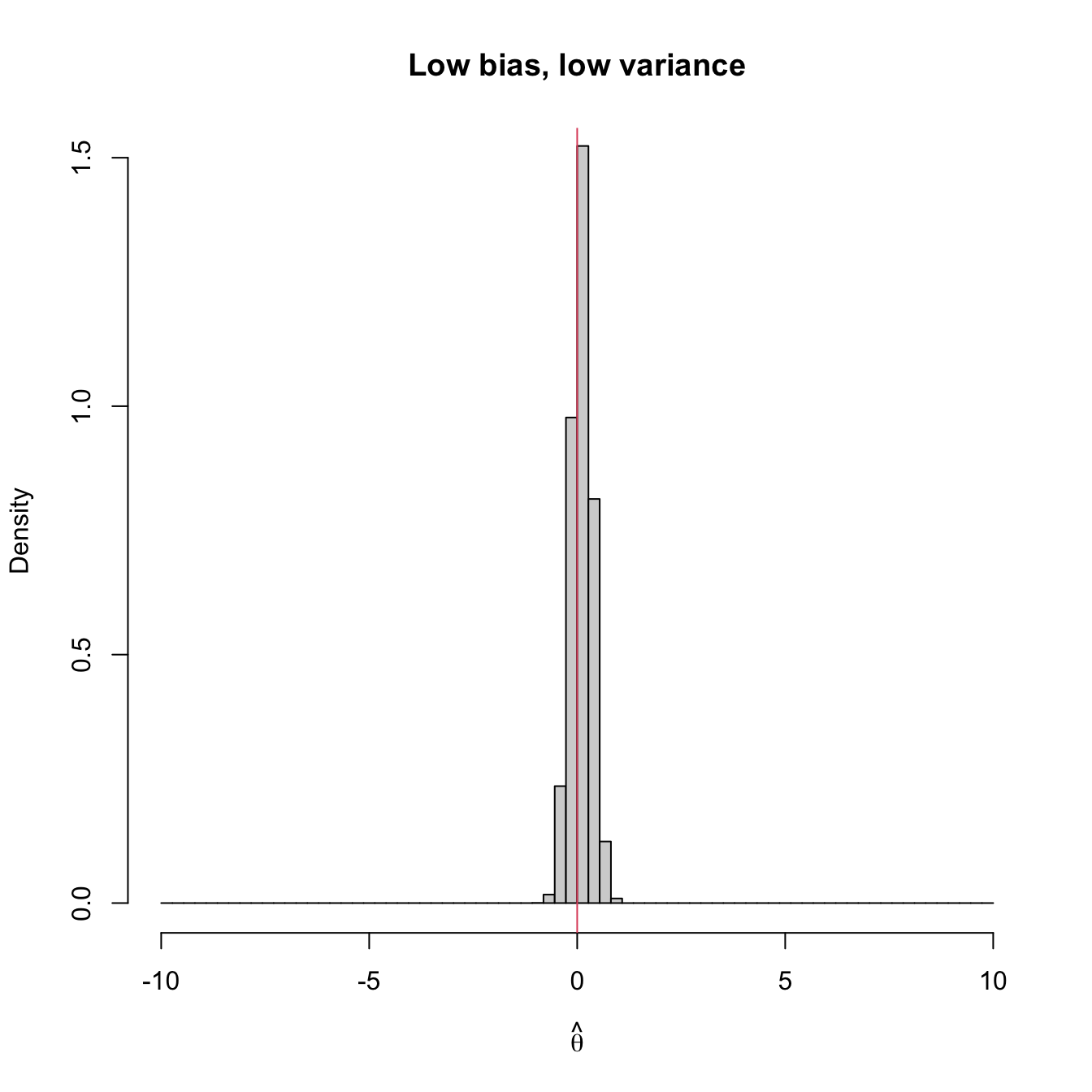
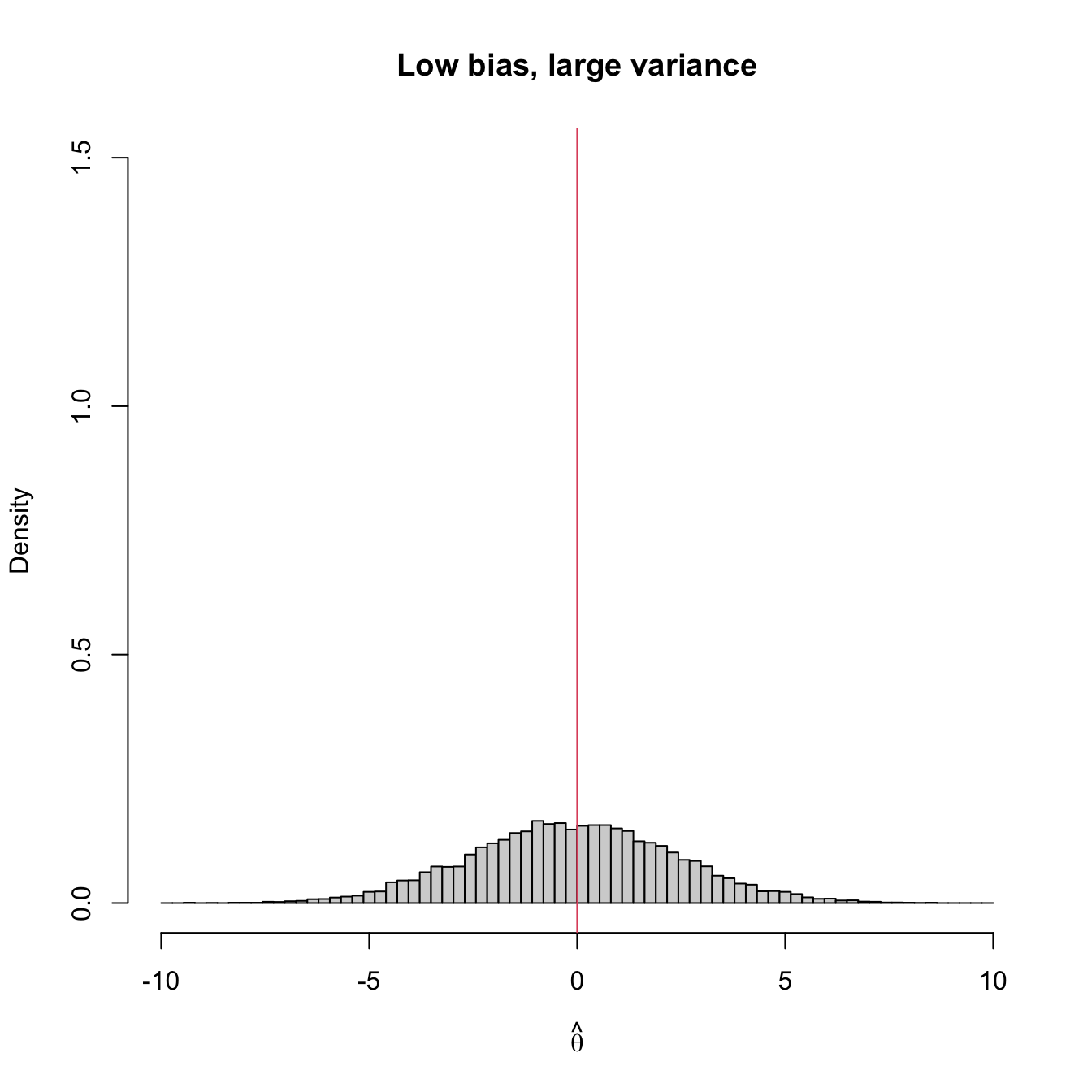
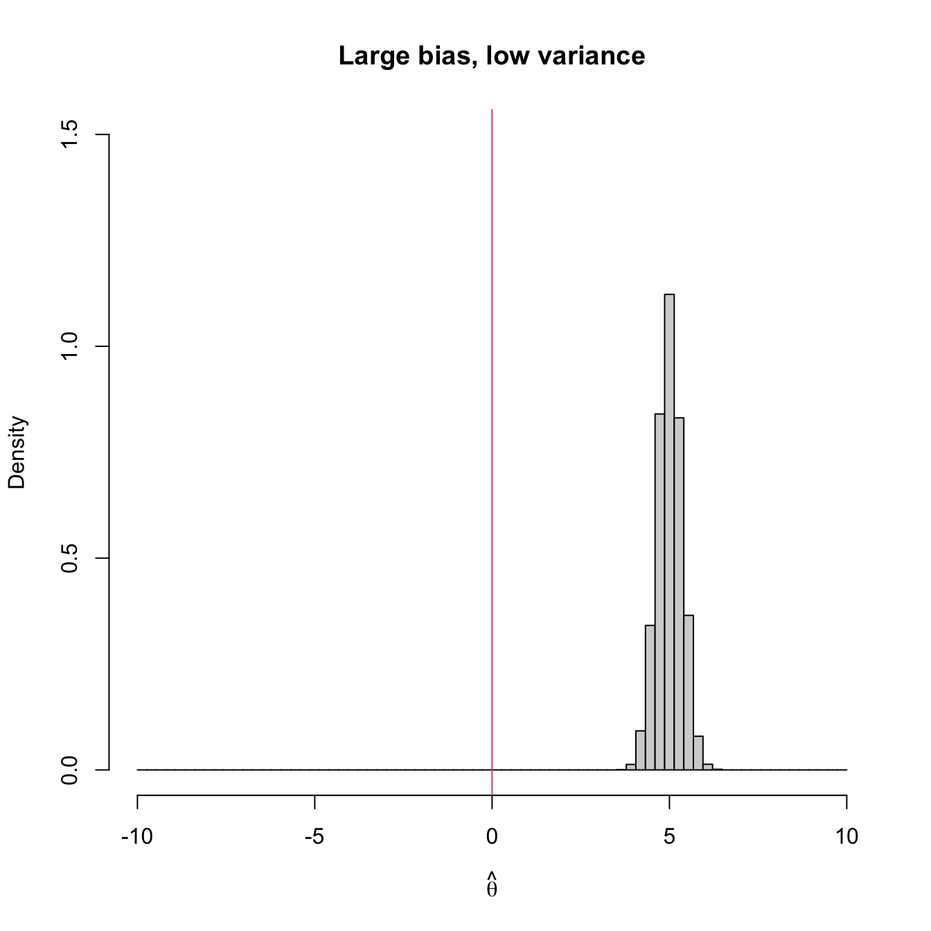
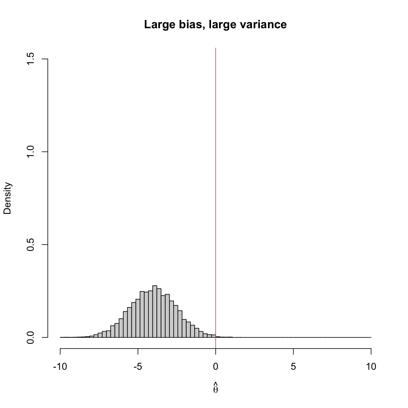
Figure 3.2: Bias and variance of an estimator \(\hat{\theta},\) represented by the positioning of its simulated distribution (histogram) with respect to the target parameter \(\theta=0\) (red vertical line).

Example 3.5 Let us compute the MSE of the sample variance \(S^2\) and the sample quasivariance \(S'^2\) when estimating the population variance \(\sigma^2\) of a normal rv (this assumption is fundamental for obtaining the expression for the variance of \(S^2\) and \(S'^2\)).

In Exercise 2.19 we saw that, for a normal population,

\[\begin{align*} \mathbb{E}[S^2]&=\frac{n-1}{n}\sigma^2, & \mathbb{V}\mathrm{ar}[S^2]&=\frac{2(n-1)}{n^2}\sigma^4,\\ \mathbb{E}[S'^2]&=\sigma^2, & \mathbb{V}\mathrm{ar}[S'^2]&=\frac{2}{n-1}\sigma^4. \end{align*}\]

Therefore, the bias of \(S^2\) is

\[\begin{align*} \mathrm{Bias}[S^2]=\frac{n-1}{n}\sigma^2-\sigma^2=-\frac{1}{n}\sigma^2<0 \end{align*}\]

and the MSE of \(S^2\) for estimating \(\sigma^2\) is

\[\begin{align*} \mathrm{MSE}[S^2]=\mathrm{Bias}^2[S^2]+\mathbb{V}\mathrm{ar}[S^2]=\frac{1}{n^2}\sigma^4+\frac{2(n-1)}{n^2}\sigma^4= \frac{2n-1}{n^2}\sigma^4. \end{align*}\]

Replicating the calculations for the sample quasivariance, we have that

\[\begin{align*} \mathrm{MSE}[S'^2]=\mathbb{V}\mathrm{ar}[S'^2]=\frac{2}{n-1}\sigma^4. \end{align*}\]

Since \(n>1,\) we have

\[\begin{align*} \frac{2}{n-1}>\frac{2n-1}{n^2} \end{align*}\]

and, as a consequence,

\[\begin{align*} \mathrm{MSE}[S'^2]>\mathrm{MSE}[S^2]. \end{align*}\]

The bottom line is clear: despite \(S'^2\) being unbiased and \(S^2\) not, for normal populations \(S^2\) has lower MSE than \(S'^2\) when estimating \(\sigma^2.\) Therefore, \(S^2\) is better than \(S'^2\) in terms of MSE for estimating \(\sigma^2\) in normal populations. This highlights that unbiased estimators are not always to be preferred in terms of the MSE!

The use of unbiased estimators is convenient when the sample size \(n\) is large, since in those cases the variance tends to be small. However, when \(n\) is small, the bias is usually very small compared with the variance, so a smaller MSE can be obtained by focusing on decreasing the variance. On the other hand, it is possible that, for a parameter and a given sample, there is no unbiased estimator, as the following example shows.

Example 3.6 The next game is presented to us. We have to pay \(6\) euros in order to participate and the payoff is \(12\) euros if we obtain two heads in two tosses of a coin with heads probability \(p.\) We receive \(0\) euros otherwise. We are allowed to perform a test toss for estimating the value of the success probability \(\theta=p^2.\)

In the coin toss we observe the value of the rv

\[\begin{align*} X_1=\begin{cases} 1 & \text{if heads},\\ 0 & \text{if tails}. \end{cases} \end{align*}\]

We know that \(X_1\sim \mathrm{Ber}(p).\) Let

\[\begin{align*} \hat{\theta}:=\begin{cases} \hat{\theta}_1 & \text{if} \ X_1=1,\\ \hat{\theta}_0 & \text{if} \ X_1=0. \end{cases} \end{align*}\]

be an estimator of \(\theta=p^2,\) where \(\hat{\theta}_0\) and \(\hat{\theta}_1\) are to be determined. Its expectation is

\[\begin{align*} \mathbb{E}\big[\hat{\theta}\big]=\hat{\theta}_1\times p+\hat{\theta}_0\times (1-p), \end{align*}\]

which is different from \(p^2\) for any estimator \(\hat{\theta};\) \(\mathbb{E}\big[\hat{\theta}\big]=p^2\) will be achieved if \(\hat{\theta}_1=p\) and \(\hat{\theta}_0=0,\) which is not allowed since \(\hat{\theta}\) can only depend on the sample and not on the unknown parameter. Therefore, for any given sample of size \(n=1\) there does not exist any unbiased estimator of \(p^2.\)

3.2 Invariant estimators

Let us introduce the concept of invariance with an example.

Example 3.7 The manufacturer of a given product claims that the product packages contain at least \(\theta\) grams of product. If this claim is true, then the product content within a package is distributed as \(\mathcal{U}(\theta, \theta+100).\) To check the claim of the manufacturer, a srs measuring the content was taken. The realization of this srs is \((x_1,\ldots,x_n)\) and is used to compute an estimate \(\hat{\theta}(x_1,\ldots,x_n).\) But, after computing the estimate, it is discovered that the scale was systematically weighing \(c\) grams less. Can we just simply correct the estimate as \(\hat{\theta}(x_1,\ldots,x_n)+c\)?

The answer to the question depends on whether the estimator verifies

\[\begin{align*} \hat{\theta}(x_1+c,\ldots,x_n+c)=\hat{\theta}(x_1,\ldots,x_n)+c. \end{align*}\]

If this is not the case, then we will need to compute \(\hat{\theta}(x_1+c,\ldots,x_n+c)\) without being able to reuse \(\hat{\theta}(x_1,\ldots,x_n).\)

Definition 3.3 (Translation-invariant estimator) An estimator \(\hat{\theta}\) is translation-invariant if, for sample realization \((x_1,\ldots,x_n)\) and any \(c\in\mathbb{R},\)

\[\begin{align*} \hat{\theta}(x_1+c,\ldots,x_n+c)=\hat{\theta}(x_1,\ldots,x_n)+c. \end{align*}\]

Example 3.8 Check that \(X_{(1)},\) \(\bar{X},\) and \((X_{(1)}+X_{(n)})/2\) are statistics invariant to translations, but that the geometric mean \((\prod_{i=1}^n X_i)^{1/n}\) and the harmonic mean \(n/\sum_{i=1}^n X_i^{-1}\) are not.

For \(X_{(1)}=\min_{1\leq i\leq n} X_i,\) we have

\[\begin{align*} \min_{1\leq i\leq n} (X_i+c)=\min_{1\leq i\leq n} (X_i)+c. \end{align*}\]

Therefore, \(X_{(1)}\) is translation-invariant. For \(\bar{X}=(1/n)\sum_{i=1}^n X_i,\)

\[\begin{align*} \frac{1}{n}\sum_{i=1}^n (X_i+c)=\frac{1}{n}\left[\sum_{i=1}^n X_i+nc\right]=\frac{1}{n}\sum_{i=1}^n X_i+c=\bar{X}+c, \end{align*}\]

so \(\bar{X}\) is translation-invariant too. We now check \((X_{(1)}+X_{(n)})/2\):

\[\begin{align*} \frac{1}{2}\left[\min_{1\leq i\leq n}(X_i+c)+\max_{1\leq i\leq n}(X_i+c)\right]&=\frac{1}{2}\left[\min_{1\leq i\leq n}X_i+\max_{1\leq i\leq n}X_i+2c\right]\\ &=\frac{1}{2}\left(X_{(1)}+X_{(n)}\right)+c. \end{align*}\]

To see that neither the geometric nor the harmonic means are invariant to translations, we only need to find counterexamples. For that, consider the sample realization \((x_1,x_2,x_3)=(1,2,3).\) For these data, the geometric and harmonic means are, respectively,

\[\begin{align*} \left[\prod_{i=1}^n x_i\right]^{1/n}&=(1\times 2\times 3)^{1/3}=6^{1/3}=1.82,\\ \frac{n}{\sum_{i=1}^n x_i^{-1}}&=\frac{3}{1+\frac{1}{2}+\frac{1}{3}}=\frac{18}{11}=1.64. \end{align*}\]

However, if we take \(c=1\):

\[\begin{align*} \left[\prod_{i=1}^n (x_i+c)\right]^{1/n}&=(2\times 3\times 4)^{1/3}=2.88\neq 1.82+1,\\ \frac{n}{\sum_{i=1}^n (x_i+c)^{-1}}&=\frac{3}{\frac{1}{2}+\frac{1}{3}+\frac{1}{4}}=\frac{36}{13}=2.77\neq 1.64+1, \end{align*}\]

and we see that none of these statistics is translation-invariant.

Example 3.9 A woman always arrives to the bus stop at the same hour. She wishes to estimate the maximum time waiting for the bus, knowing that the waiting time is distributed as \(\mathcal{U}(0,\theta).\) For that purpose, she times the waiting times during \(n\) days and obtains a realization of a srs, \((x_1,\ldots,x_n),\) measured in seconds. Based on that sample, she obtains an estimate of the maximum waiting time \(\hat{\theta}(x_1,\ldots,x_n)\) in seconds. If she wants to convert the result to minutes, can she just compute \(\hat{\theta}(x_1,\ldots,x_n)/60\)?

The answer depends on whether the estimator satisfies

\[\begin{align*} \hat{\theta}(x_1/60,\ldots,x_n/60)=\hat{\theta}(x_1,\ldots,x_n)/60. \end{align*}\]

If this is not the case, then she will need to compute \(\hat{\theta}(x_1/60,\ldots,x_n/60).\)

Definition 3.4 (Scale-invariant estimators) An estimator \(\hat{\theta}\) is scale-invariant if, for sample realization \((x_1,\ldots,x_n)\) and any \(c>0,\)

\[\begin{align*} \hat{\theta}(cx_1,\ldots,cx_n)=c\,\hat{\theta}(x_1,\ldots,x_n). \end{align*}\]

Example 3.10 Check that \(\bar{X}\) and \(X_{(n)}\) are scale-invariant estimators and that \(\log((1/n)\sum_{i=1}^n\exp({X_i}))\) and \(X_{(n)}/X_{(1)}\) are not.

3.3 Consistent estimators

The concept of consistency is related with the sample size \(n.\) Assume that \(X\) is a rv with induced probability \(\mathbb{P}(\cdot;\theta),\) \(\theta\in\Theta,\) and that \((X_1,\ldots,X_n)\) is a srs of \(X.\) Take an estimator \(\hat{\theta}\equiv\hat{\theta}(X_1,\ldots,X_n),\) where we have emphasized the dependence of the estimator on the srs. Of course \(\hat{\theta}\) depends on \(n\) and, to remark that, we will also denote the estimator by \(\hat{\theta}_n.\) The question now is: what happens with the distribution of this estimator as the sample size increases? Is its distribution going to be more concentrated around the true value \(\theta\)?

We will study different concepts of consistency, all of them taking into account the distribution of \(\hat{\theta}.\) The first concept we will see tells us that an estimator is consistent in probability if the probability of \(\hat{\theta}\) being far away from \(\theta\) decays as \(n\to\infty.\)

Example 3.11 Let \(X\sim \mathcal{N}(\mu,\sigma^2).\) Let us see how the distribution of \(\bar{X}-\mu\) changes as \(n\) increases, for \(\sigma=2.\)

We know from Theorem 2.1 that

\[\begin{align*} Z=\frac{\bar{X}-\mu}{\sigma/\sqrt{n}}\sim\mathcal{N}(0,1). \end{align*}\]

From that result, we have computed below the probabilities \(\mathbb{P}\left(\vert\bar{X}_n-\mu\vert>\varepsilon\right)=2\mathbb{P}\left(Z>\frac{\varepsilon}{\sigma/\sqrt{n}}\right)\) for \(\varepsilon_1=1\) and \(\varepsilon_2=0.5.\)

\(n\)	\(\bar{X}_n\)	\(\mathbb{P}\left(\vert\bar{X}_n-\mu\vert>1\right)\)	\(\mathbb{P}\left(\vert\bar{X}_n-\mu\vert>0.5\right)\)
\(1\)	\(X_1\)	\(0.6171\)	\(0.8026\)
\(2\)	\(\sum_{i=1}^2X_i/2\)	\(0.4795\)	\(0.7237\)
\(3\)	\(\sum_{i=1}^3X_i/3\)	\(0.3865\)	\(0.6650\)
\(10\)	\(\sum_{i=1}^{10} X_i/10\)	\(0.1138\)	\(0.4292\)
\(20\)	\(\sum_{i=1}^{20} X_i/20\)	\(0.0253\)	\(0.2636\)
\(50\)	\(\sum_{i=1}^{50} X_i/50\)	\(0.0004\)	\(0.0771\)

Observe that \(\bar{X}_n\) is a sequence of estimators of \(\mu\) indexed by \(n.\) Moreover, the probabilities shown in the table also form a sequence. This sequence of probabilities decreases to zero as we increase the sample size \(n.\) This convergence towards zero happens irrespective of the value of \(\varepsilon,\) despite the sequence of probabilities for \(\varepsilon_2\) being larger than the one for \(\varepsilon_1,\) for each \(n,\) since \(\varepsilon_2\leq \varepsilon_1.\) Figure 3.3 shows the evolution of the “\(\bar{X}_n\) is \(\varepsilon\) units far away from \(\mu\)” probabilities for several \(\varepsilon\)’s.

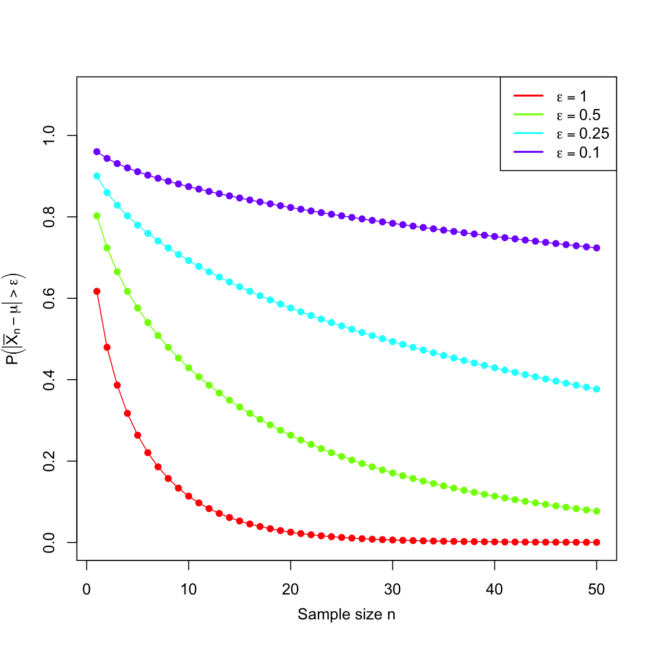
Figure 3.3: Probability sequences \(n\mapsto\mathbb{P}\left(\vert\bar{X}_n-\mu\vert>\varepsilon\right)\) for a \(\mathcal{N}(\mu,\sigma^2)\) with \(\sigma=2\).

Then, an estimator \(\hat{\theta}\) for \(\theta\) is consistent in probability when the probabilities of \(\hat{\theta}\) and \(\theta\) differing more than \(\varepsilon>0\) decrease as \(n\to\infty.\) Or, equivalently, when the probabilities of \(\hat{\theta}\) and \(\theta\) being closer than \(\varepsilon\) grow as \(n\) increases. This must happen for any \(\varepsilon>0.\) If this is true, then the distribution of \(\hat{\theta}\) becomes more and more concentrated about \(\theta.\)

Definition 3.5 (Consistency in probability) Let \(X\) be a rv with induced probability \(\mathbb{P}(\cdot;\theta).\) Let \((X_1,\ldots,X_n)\) be a srs of \(X\) and let \(\hat{\theta}_n\equiv\hat{\theta}_n(X_1,\ldots,X_n)\) be an estimator of \(\theta.\) The sequence \(\{\hat{\theta}_n:n\in\mathbb{N}\}\) is said to be consistent in probability (or consistent) for \(\theta,\) if

\[\begin{align*} \forall \varepsilon>0, \quad \lim_{n\to\infty} \mathbb{P}\big(|\hat{\theta}_n-\theta|>\varepsilon\big)=0. \end{align*}\]

We simply say that the estimator \(\hat{\theta}_n\) is consistent in probability to indicate that the sequence \(\{\hat{\theta}_n:n\in\mathbb{N}\}\) is consistent in probability.

Example 3.12 Let \(X\sim\mathcal{U}(0,\theta)\) and let \((X_1,\ldots,X_n)\) be a srs of \(X.\) Show that the estimator \(\hat{\theta}_n=X_{(n)}\) is consistent in probability for \(\theta.\)

We take \(\varepsilon>0\) and compute the limit of the probability given in Definition 3.5. Since \(\theta \geq X_i,\) \(i=1,\ldots,n,\) we have that

\[\begin{align*} \mathbb{P}\big(|\hat{\theta}_n-\theta|>\varepsilon\big)=\mathbb{P}(\theta-X_{(n)}>\varepsilon)=\mathbb{P}\left(X_{(n)}<\theta-\varepsilon\right)=F_{X_{(n)}}(\theta-\varepsilon). \end{align*}\]

If \(\varepsilon>\theta,\) then \(\theta-\varepsilon<0\) and therefore \(F_{X_{(n)}}(\theta-\varepsilon)=0.\) For \(\varepsilon\leq\theta,\) the cdf evaluated at \(\theta-\varepsilon\) is not zero. Using Example 3.3:

\[\begin{align*} F_{X_{(n)}}(x)=\left(F_X(x)\right)^n=\left(\frac{x}{\theta}\right)^n, \quad x\in(0,\theta). \end{align*}\]

Considering the value of such distribution at \(\theta-\varepsilon\in [0,\theta),\) we get

\[\begin{align*} F_{X_{(n)}}(\theta-\varepsilon)=\left(\frac{\theta-\varepsilon}{\theta}\right)^n=\left(1-\frac{\varepsilon}{\theta}\right)^n. \end{align*}\]

Then, taking the limit as \(n\to\infty\) and noting that \(\varepsilon<\theta,\) we have

\[\begin{align*} \lim_{n\to\infty} \mathbb{P}\big(|\hat{\theta}_n-\theta|>\varepsilon\big)=\lim_{n\to\infty}\left(1-\frac{\varepsilon}{\theta}\right)^n=0. \end{align*}\]

We have shown that \(\hat{\theta}_n=X_{(n)}\) is consistent in probability for \(\theta.\)

The concept of consistency in probability of a sequence of estimators can be extended to general sequences of rv’s. This gives an important type of convergence of rv’s, the convergence in probability.³³

Definition 3.6 (Convergence in probability) A sequence \(\{X_n:n\in\mathbb{N}\}\) of rv’s defined over the same measurable space \((\Omega,\mathcal{A},\mathbb{P})\) is said to converge in probability to another rv \(X,\) and is denoted by

\[\begin{align*} X_n \stackrel{\mathbb{P}}{\longrightarrow} X, \end{align*}\]

if the following statement holds:

\[\begin{align*} \forall \varepsilon>0, \quad \lim_{n\to\infty} \mathbb{P}(|X_n-X|>\varepsilon)=0, \end{align*}\]

where here \(\mathbb{P}\) stands for the joint induced probability function of \(X_n\) and \(X.\)

The following definition establishes another type of consistency that is stronger than (in the sense that it implies, but is not implied by) consistency in probability.

Definition 3.7 (Consistency in squared mean) A sequence of estimators \(\{\hat{\theta}_n:n\in\mathbb{N}\}\) is consistent in squared mean for \(\theta\) if

\[\begin{align*} \lim_{n\to\infty}\mathrm{MSE}\big[\hat{\theta}_n\big]=0, \end{align*}\]

or, equivalently, if

\[\begin{align*} \lim_{n\to\infty} \mathrm{Bias}\big[\hat{\theta}_n\big]=0 \quad \text{and}\quad \lim_{n\to\infty} \mathbb{V}\mathrm{ar}\big[\hat{\theta}_n\big]=0. \end{align*}\]

Example 3.13 In a \(\mathcal{U}(0,\theta)\) population, let us check if \(\hat{\theta}_n=X_{(n)}\) is consistent in squared mean for \(\theta.\)

The MSE of \(\hat{\theta}_n\) is given by³⁴

\[\begin{align*} \mathrm{MSE}\big[\hat{\theta}_n\big]=\mathbb{E}\big[(\hat{\theta}_n-\theta)^2\big]=\mathbb{E}\big[\hat{\theta}_n^2-2\theta\hat{\theta}_n+\theta^2\big]. \end{align*}\]

Therefore, we have to compute the expectation and variance of \(\hat{\theta}_n=X_{(n)}.\) Example 3.3 gave the density and expectation of \(\hat{\theta}_n=X_{(n)}\):

\[\begin{align*} f_{\hat{\theta}_n}(x)=\frac{n}{\theta}\left(\frac{x}{\theta}\right)^{n-1}, \quad x\in(0,\theta), \quad \mathbb{E}\big[\hat{\theta}_n\big]=\frac{n}{n+1}\theta. \end{align*}\]

It remains to compute

\[\begin{align*} \mathbb{E}\big[\hat{\theta}_n^2\big]&=\int_0^{\theta} x^2 \frac{n}{\theta}\left(\frac{x}{\theta}\right)^{n-1}\,\mathrm{d}x\\ &=\frac{n}{\theta^n} \int_0^{\theta} x^{n+1}\,\mathrm{d}x=\frac{n}{\theta^n}\frac{\theta^{n+2}}{n+2}= \frac{n\theta^2}{n+2}. \end{align*}\]

Then, the MSE is

\[\begin{align*} \mathrm{MSE}\big[\hat{\theta}_n\big]=\left(1-\frac{2n}{n+1}+\frac{n}{n+2}\right)\theta^2. \end{align*}\]

Taking the limit as \(n\to\infty,\) we obtain

\[\begin{align*} \lim_{n\to\infty} \mathrm{MSE}\big[\hat{\theta}_n\big]=0, \end{align*}\]

so \(\hat{\theta}_n=X_{(n)}\) is consistent in squared mean (even if it is biased).

From the previous definition we deduce automatically the following result.

Corollary 3.1 Assume that \(\hat{\theta}_n\) is unbiased for \(\theta,\) for all \(n\in\mathbb{N}.\) Then \(\hat{\theta}_n\) is consistent in squared mean for \(\theta\) if and only if

\[\begin{align*} \lim_{n\to\infty} \mathbb{V}\mathrm{ar}\big[\hat{\theta}_n\big]=0. \end{align*}\]

The next result shows that consistency in squared mean is stronger than consistency in probability.

Theorem 3.1 (Consistency in squared mean implies consistency in probability) Consistency in squared mean of an estimator \(\hat{\theta}_n\) of \(\theta\) implies consistency in probability of \(\hat{\theta}_n\) to \(\theta.\)

Proof (Proof of Theorem 3.1). We first assume that \(\hat{\theta}_n\) is a consistent estimator of \(\theta,\) in squared mean. Then, taking \(\varepsilon>0\) and applying Markov’s inequality (Proposition 3.2) for \(X=\hat{\theta}_n-\theta\) and \(k=\varepsilon,\) we obtain

\[\begin{align*} 0\leq \mathbb{P}\big(|\hat{\theta}_n-\theta| \geq \varepsilon\big)\leq \frac{\mathbb{E}\big[(\hat{\theta}_n-\theta)^2\big]}{\varepsilon^2}=\frac{\mathrm{MSE}\big[\hat{\theta}_n\big]}{\varepsilon^2}. \end{align*}\]

The right hand side tends to zero as \(n\to\infty\) because of the consistency in squared mean. Then,

\[\begin{align*} \lim_{n\to\infty} \mathbb{P}\big(|\hat{\theta}_n-\theta| \geq\varepsilon\big)=0, \end{align*}\]

and this happens for any \(\varepsilon>0.\)

Combining Corollary 3.1 and Theorem 3.1, the task of proving the consistency in probability of an unbiased estimator is notably simplified: it is only required to compute the limit of its variance, a much simpler task than directly employing Definition 3.5. If the estimator is biased, proving the consistency in probability of \(\hat{\theta}_n\) to \(\theta\) can be done by checking that:

\[\begin{align*} \lim_{n\to\infty} \mathbb{E}\big[\hat{\theta}_n\big]=\theta,\quad \lim_{n\to\infty} \mathbb{V}\mathrm{ar}\big[\hat{\theta}_n\big]=0. \end{align*}\]

Example 3.14 Let \((X_1,\ldots,X_n)\) be a srs of a rv with mean \(\mu\) and variance \(\sigma^2.\) Consider the following estimators of \(\mu\):

\[\begin{align*} \hat{\mu}_1=\frac{X_1+X_2}{2},\quad \hat{\mu}_2=\frac{X_1}{4}+\frac{X_2+\cdots + X_{n-1}}{2(n-2)}+\frac{X_n}{4},\quad \hat{\mu}_3=\bar{X}. \end{align*}\]

Which one is unbiased? Which one is consistent in probability for \(\mu\)?

The expectations of these estimators are

\[\begin{align*} \mathbb{E}\big[\hat{\mu}_1\big]=\mathbb{E}\big[\hat{\mu}_2\big]=\mathbb{E}\big[\hat{\mu}_3\big]=\mu, \end{align*}\]

so all of them are unbiased. Now, to check whether they are consistent in probability or not, it only remains to check whether their variances tend to zero. But their variances are respectively given by

\[\begin{align*} \mathbb{V}\mathrm{ar}\big[\hat{\mu}_1\big]=\frac{\sigma^2}{2}, \quad \mathbb{V}\mathrm{ar}\big[\hat{\mu}_2\big]=\frac{n\sigma^2}{8(n-2)}, \quad \mathbb{V}\mathrm{ar}\big[\hat{\mu}_3\big]=\frac{\sigma^2}{n}. \end{align*}\]

Unlike the variances of \(\hat{\mu}_1\) and \(\hat{\mu}_2,\) we can see that the variance of \(\hat{\mu}_3\) converges to zero, which means that we can only guarantee that \(\hat{\mu}_3\) is consistent in probability for \(\mu.\) The estimators \(\hat{\mu}_1\) and \(\hat{\mu}_2\) are not consistent in square mean, so they are unlikely to be consistent in probability.³⁵

The Law of the Large Numbers (LLN) stated below follows by straightforward application of the previous results.

Theorem 3.2 (Law of the Large Numbers) Let \((X_1,\ldots,X_n)\) be a srs of a rv \(X\) with mean \(\mu\) and variance \(\sigma^2<\infty.\) Then,

\[\begin{align*} \bar{X} \stackrel{\mathbb{P}}{\longrightarrow} \mu. \end{align*}\]

The above LLN ensures that, by averaging many iid observations of a rv \(X,\) we can get arbitrarily close to the true mean \(\mu=\mathbb{E}[X].\) For example, if we were interested in knowing the average weight of an animal, by taking many independent measurements of the weight and averaging them we will get a value very close to the true weight.

Example 3.15 Let \(Y\sim \mathrm{Bin}(n,p).\) Let us see that \(\hat{p}=Y/n\) is consistent in probability for \(p.\)

We use the representation \(Y=n\bar{X}=\sum_{i=1}^n X_i,\) where the rv’s \(X_i\) are iid \(\mathrm{Ber}(p),\) with

\[\begin{align*} \mathbb{E}[X_i]=p,\quad \mathbb{V}\mathrm{ar}[X_i]=p(1-p)<\infty. \end{align*}\]

This means that the sample proportion \(\hat{p}\) is actually a sample mean:

\[\begin{align*} \hat{p}=\frac{\sum_{i=1}^n X_i}{n}=\bar{X}. \end{align*}\]

Applying the LLN, we get that \(\hat{p}=\bar{X}\) converges in probability to \(p=\mathbb{E}[X_i].\)

The LLN implies the following result, giving the condition under which the sample moments are consistent in probability for the population moments.

Corollary 3.2 (Consistency in probability of the sample moments) Let \(X\) be a rv with \(k\)-th population moment \(\alpha_k=\mathbb{E}[X^k]\) and such that \(\alpha_{2k}=\mathbb{E}[X^{2k}]<\infty.\) Let \((X_1,\ldots,X_n)\) be a srs of \(X,\) with \(k\)-th sample moment \(a_k=\frac{1}{n}\sum_{i=1}^n X_i^k.\) Then,

\[\begin{align*} a_k\stackrel{\mathbb{P}}{\longrightarrow} \alpha_k. \end{align*}\]

Proof (Proof of Corollary 3.2). The proof is straightforward by taking \(Y_i:=X_i^k,\) \(i=1,\ldots,n,\) in such a way that \((Y_1,\ldots,Y_n)\) represents a srs of a rv \(Y\) with mean \(\mathbb{E}[Y]=\mathbb{E}[X^k]=\alpha_k\) and variance \(\mathbb{V}\mathrm{ar}[Y]=\mathbb{E}[(X^k-\alpha_k)^2]=\alpha_{2k}-\alpha_k^2<\infty.\) Then by the LLN, we have that \(a_k=\frac{1}{n}\sum_{i=1}^n Y_i\stackrel{\mathbb{P}}{\longrightarrow} \alpha_k.\)

The following theorem states that any continuous transformation \(g\) of an estimator \(\hat{\theta}_n\) that is consistent in probability to \(\theta\) is also consistent for the transformed parameter \(g(\theta).\)

Theorem 3.3 (Version of the continuous mapping theorem)

1. Let \(\hat{\theta}_n\stackrel{\mathbb{P}}{\longrightarrow} \theta\) and let \(g\) be a function that is continuous at \(\theta.\) Then,

\[\begin{align*} g(\hat{\theta}_n)\stackrel{\mathbb{P}}{\longrightarrow} g(\theta). \end{align*}\]

2. Let \(\hat{\theta}_n\stackrel{\mathbb{P}}{\longrightarrow} \theta\) and \(\hat{\theta}_n'\stackrel{\mathbb{P}}{\longrightarrow} \theta'.\) Let \(g\) be a bivariate function that is continuous at \((\theta,\theta').\) Then,

\[\begin{align*} g\left(\hat{\theta}_n,\hat{\theta}_n'\right)\stackrel{\mathbb{P}}{\longrightarrow}g\left(\theta,\theta'\right). \end{align*}\]

Proof (Proof of Theorem 3.3). We show only part i. Part ii follows from analogous arguments.

Due to the continuity of \(g\) at \(\theta,\) for all \(\varepsilon>0,\) there exists a \(\delta=\delta(\varepsilon)>0\) such that

\[\begin{align*} |x-\theta|<\delta\implies \left|g(x)-g(\theta)\right|<\varepsilon. \end{align*}\]

Hence, for any fixed \(n,\) it holds

\[\begin{align*} 1\geq \mathbb{P}\left(\left|g(\hat{\theta}_n)-g(\theta)\right|\leq \varepsilon\right)\geq \mathbb{P}\big(|\hat{\theta}_n-\theta| \leq \delta\big). \end{align*}\]

Therefore, if \(\hat{\theta}_n\stackrel{\mathbb{P}}{\longrightarrow} \theta,\) then

\[\begin{align*} \lim_{n\to\infty} \mathbb{P}\big(|\hat{\theta}_n-\theta| \leq \delta\big)=1, \end{align*}\]

and, as a consequence,

\[\begin{align*} \lim_{n\to\infty} \mathbb{P}\left(\left|g(\hat{\theta}_n)-g(\theta)\right|\leq \varepsilon\right)=1. \end{align*}\]

The following corollary readily follows from Theorem 3.3, but it makes explicit some of the possible algebraic operations that preserve the convergence in probability.

Corollary 3.3 (Algebra of the convergence in probability) Assume that \(\hat{\theta}_n\stackrel{\mathbb{P}}{\longrightarrow} \theta\) and \(\hat{\theta}_n'\stackrel{\mathbb{P}}{\longrightarrow} \theta'.\) Then:

1. \(\hat{\theta}_n+\hat{\theta}_n' \stackrel{\mathbb{P}}{\longrightarrow} \theta+\theta'.\)
2. \(\hat{\theta}_n\hat{\theta}_n' \stackrel{\mathbb{P}}{\longrightarrow}\theta\theta'.\)
3. \(\hat{\theta}_n/\hat{\theta}_n' \stackrel{\mathbb{P}}{\longrightarrow} \theta/\theta'\) if \(\theta'\neq 0.\)
4. Let \(a_n\to a\) be a deterministic sequence. Then \(a_n\hat{\theta}_n\stackrel{\mathbb{P}}{\longrightarrow} a\theta.\)

Example 3.16 (Consistency in probability of the sample quasivariance) Let \((X_1,\ldots,X_n)\) be a srs of a rv \(X\) with the following finite moments:

\[\begin{align*} \mathbb{E}[X]=\mu, \quad \mathbb{E}[X^2]=\alpha_2, \quad \mathbb{E}[X^4]=\alpha_4. \end{align*}\]

Its variance is therefore \(\mathbb{V}\mathrm{ar}[X]=\alpha_2-\mu^2=\sigma^2.\) Let us check that \(S'^2\stackrel{\mathbb{P}}{\longrightarrow} \sigma^2.\)

\(S'^2\) can be written as

\[\begin{align*} S'^2=\frac{n}{n-1}\left(\frac{1}{n}\sum_{i=1}^n X_i^2-{\bar{X}}^2\right). \end{align*}\]

Now, by the LLN,

\[\begin{align*} \bar{X}\stackrel{\mathbb{P}}{\longrightarrow} \mu. \end{align*}\]

Firstly, applying part ii of Corollary 3.3, we obtain

\[\begin{align} \bar{X}^2\stackrel{\mathbb{P}}{\longrightarrow} \mu^2. \tag{3.3} \end{align}\]

Secondly, the rv’s \(Y_i:=X_i^2\) have mean \(\mathbb{E}[Y_i]=\mathbb{E}[X_i^2]=\alpha_2\) and variance \(\mathbb{V}\mathrm{ar}[Y_i]=\mathbb{E}[X_i^4]-\mathbb{E}[X_i^2]=\alpha_4-\alpha_2<\infty,\) \(i=1,\ldots,n.\) Applying the LLN to \((Y_1,\ldots,Y_n),\) we obtain

\[\begin{align} \bar{Y}=\frac{1}{n}\sum_{i=1}^n X_i^2 \stackrel{\mathbb{P}}{\longrightarrow} \alpha_2.\tag{3.4} \end{align}\]

Applying now part i of Corollary 3.3 to (3.3) and (3.4), we get

\[\begin{align*} \frac{1}{n}\sum_{i=1}^n X_i^2-{\bar{X}}^2\stackrel{\mathbb{P}}{\longrightarrow} \alpha_2-\mu^2=\sigma^2. \end{align*}\]

Observe that we have just proved consistency in probability for the sample variance \(S^2.\) Applying part iv of Corollary 3.3 with the following deterministic sequence

\[\begin{align*} \lim_{n\to\infty}\frac{n}{n-1}=1, \end{align*}\]

we conclude that

\[\begin{align*} S'^2\stackrel{\mathbb{P}}{\longrightarrow} \sigma^2. \end{align*}\]

The next theorem delivers the asymptotic normality of the \(T\) statistic that was used in Section 2.2.3 for normal populations. This theorem will be rather useful for deriving the asymptotic distribution (via convergence in distribution) of an estimator that is affected by a nuisance factor converging to \(1\) in probability.

Theorem 3.4 (Version of Slutsky's Theorem) Let \(U_n\) and \(W_n\) be two rv’s that satisfy, respectively,

\[\begin{align*} U_n\stackrel{d}{\longrightarrow} \mathcal{N}(0,1),\quad W_n\stackrel{\mathbb{P}}{\longrightarrow} 1. \end{align*}\]

Then,

\[\begin{align*} \frac{U_n}{W_n} \stackrel{d}{\longrightarrow} \mathcal{N}(0,1). \end{align*}\]

Example 3.17 Let \((X_1,\ldots,X_n)\) be a srs of a rv \(X\) with \(\mathbb{E}[X]=\mu\) and \(\mathbb{V}\mathrm{ar}[X]=\sigma^2.\) Show that:

\[\begin{align*} T=\frac{\bar{X}-\mu}{S'/\sqrt{n}}\stackrel{d}{\longrightarrow} \mathcal{N}(0,1). \end{align*}\]

In Example 3.16 we saw \(S'^2\stackrel{\mathbb{P}}{\longrightarrow} \sigma^2.\) Employing part iv in Corollary 3.3, it follows that

\[\begin{align*} \frac{S'^2}{\sigma^2} \stackrel{\mathbb{P}}{\longrightarrow} 1. \end{align*}\]

Taking square root (a continuous function at \(1\)) in Theorem 3.3, we have

\[\begin{align*} \frac{S'}{\sigma} \stackrel{\mathbb{P}}{\longrightarrow} 1. \end{align*}\]

In addition, by the CLT, we know that

\[\begin{align*} U_n=\frac{\bar{X}-\mu}{\sigma/\sqrt{n}}\stackrel{d}{\longrightarrow} \mathcal{N}(0,1). \end{align*}\]

Finally, applying Theorem 3.4 to \(U_n\) and \(W_n=S'/\sigma,\) we get

\[\begin{align*} \frac{\bar{X}-\mu}{S'/\sqrt{n}}=\frac{U_n}{W_n} \stackrel{d}{\longrightarrow} \mathcal{N}(0,1). \end{align*}\]

Example 3.18 Let \(X_1,\ldots,X_n\) be iid rv’s with distribution \(\mathrm{Ber}(p).\) Prove that the sample proportion, \(\hat{p}=\bar{X},\) satisfies

\[\begin{align*} \frac{\hat{p}-p}{\sqrt{\hat{p}(1-\hat{p})/n}}\stackrel{d}{\longrightarrow} \mathcal{N}(0,1). \end{align*}\]

Similarly as in Example 2.15, applying the CLT to \(\hat{p}=\bar{X},\) it readily follows that

\[\begin{align*} U_n=\frac{\hat{p}-p}{\sqrt{p(1-p)/n}}\stackrel{d}{\longrightarrow} \mathcal{N}(0,1). \end{align*}\]

Now, because of the LLN, we have

\[\begin{align*} \hat{p}\stackrel{\mathbb{P}}{\longrightarrow} p, \end{align*}\]

which, by part ii in Corollary 3.3, leads to

\[\begin{align*} \hat{p}(1-\hat{p})\stackrel{\mathbb{P}}{\longrightarrow} p(1-p). \end{align*}\]

Applying parts iii and iv in Corollary 3.3, we get

\[\begin{align*} W_n=\sqrt{\frac{\hat{p}(1-\hat{p})}{p(1-p)}}\stackrel{\mathbb{P}}{\longrightarrow} 1. \end{align*}\]

Finally, Theorem 3.4 gives

\[\begin{align*} \frac{\hat{p}-p}{\sqrt{\hat{p}(1-\hat{p})/n}}=\frac{U_n}{W_n}\stackrel{d}{\longrightarrow} \mathcal{N}(0,1). \end{align*}\]

3.4 Sufficient statistics

As we will see below, a statistic is sufficient for a parameter \(\theta\) if it collects all the useful information of the sample about \(\theta.\) In other words: if for a given sample we know the value of a sufficient statistic, then the sample does not offer any additional information about \(\theta\) and we could safely destroy it.

The following example motivates the definition of sufficiency.

Example 3.19 Assume that an experiment with two possible results, success and fail, is repeated \(n\) times, in a way that \((X_1\ldots,X_n)\) is a srs of a \(\mathrm{Ber}(p).\) If we compute the value of the statistic \(Y=\sum_{i=1}^n X_i\sim\mathrm{Bin}(n,p),\) does the sample provide any information about \(p\) in addition to that contained in the observed value of \(Y\)?

We can answer this question by computing the conditional probability of the sample given the observed value of \(Y\):

\[\begin{align*} \mathbb{P}\left(X_1=x_1,\ldots, X_n=x_n \mid Y=y\right)= \begin{cases} \frac{\mathbb{P}(X_1=x_1,\ldots, X_n=x_n)}{\mathbb{P}(Y=y)} & \text{if} \ \sum_{i=1}^n x_i=y,\\ 0 & \text{if} \ \sum_{i=1}^n x_i\neq y. \end{cases} \end{align*}\]

For the case \(\sum_{i=1}^n x_i=y,\) the above probability is given by

\[\begin{align*} \mathbb{P}\left(X_1=x_1,\ldots, X_n=x_n \mid Y=y\right) = \frac{p^y(1-p)^{n-y}} {\binom{n}{y}p^y(1-p)^{n-y}}=\frac{1}{\binom{n}{y}}, \end{align*}\]

which does not depend on \(p.\) This means that, once the number of total successes \(Y\) is known, there is no useful information left in the sample about the probability of success \(p.\) In this case, the information that remains in the sample is only about the order of appearance of the successes, which is superfluous for estimating \(p\) because trials are independent.

Definition 3.8 (Sufficient statistic) A statistic \(T=T(X_1,\ldots,X_n)\) is sufficient for \(\theta\) if the distribution of the sample given \(T,\) that is, the distribution of \((X_1,\ldots,X_n) \mid T,\) does not depend on \(\theta.\)

Remark. Observe that the previous definition implies that if \(T\) is a sufficient statistic for a parameter \(\theta,\) then \(T\) is also sufficient for any parameter \(g(\theta)\) that is function of \(\theta.\)³⁶

Given a realization of a srs \((X_1,\ldots,X_n)\) of a rv \(X\) with distribution \(F(\cdot;\theta)\) depending on an unknown parameter \(\theta,\) the likelihood of a value of \(\theta\) represents the credibility that the sample gives to that value of \(\theta.\) The likelihood is one of the most important concepts in statistics and statistical inference — it is the blood of many inferential tools with excellent properties. The likelihood is defined through the joint pmf for discrete rv’s or through the joint pdf for continuous rv’s.

Definition 3.9 (Likelihood) Let \((X_1,\ldots,X_n)\) be a srs of a rv \(X\sim F(\cdot;\theta).\) Let \(x_1,\ldots,x_n\) be a realization of the srs. If the rv’s are discrete, the likelihood of \(\theta\) for \((x_1,\ldots,x_n)\) is defined as the joint pmf of the srs evaluated at \((x_1,\ldots,x_n)\):

\[\begin{align*} \mathcal{L}(\theta;x_1,\ldots,x_n):=\mathbb{P}(X_1=x_1,\ldots,X_n=x_n;\theta)=p_{(X_1\ldots,X_n)}(x_1,\ldots,x_n;\theta). \end{align*}\]

If the rv’s are continuous, the likelihood is defined as the joint pdf of the srs evaluated at \((x_1,\ldots,x_n)\):

\[\begin{align*} \mathcal{L}(\theta;x_1,\ldots,x_n):=f_{(X_1\ldots,X_n)}(x_1,\ldots,x_n;\theta). \end{align*}\]

\(\mathcal{L}(\theta;x_1,\ldots,x_n)\) is usually regarded as a function of the parameter \(\theta,\) since the realization of the sample \((x_1,\ldots,x_n)\) is fixed. In the situation in which the rv’s are independent, the likelihood is

\[\begin{align*} \mathcal{L}(\theta;x_1,\ldots,x_n)=\begin{cases} \prod_{i=1}^n p_{X_i}(x_i;\theta) & \text{if the rv's are discrete}, \\ \prod_{i=1}^n f_{X_i}(x_i;\theta) & \text{if the rv's are continuous}. \end{cases} \end{align*}\]

The following theorem gives a simple method for checking whether a statistic is sufficient in terms of the likelihood.

Theorem 3.5 (Factorization criterion) Let \((X_1,\ldots,X_n)\) be a srs of a rv \(X\sim F(\cdot;\theta).\) The statistic \(T=T(X_1,\ldots,X_n)\) is sufficient for \(\theta\) if and only if the likelihood can be factorized in two nonnegative functions of the form

\[\begin{align*} \mathcal{L}(\theta;x_1,\ldots,x_n)=g(t,\theta)h(x_1,\ldots,x_n), \end{align*}\]

where \(g(t,\theta)\) only depends on the sample through \(t=T(x_1,\ldots,x_n)\) and \(h(x_1,\ldots,x_n)\) does not depend on \(\theta.\)

Proof (Proof of Theorem 3.5). We only prove the result for discrete rv’s.

Proof of “\(\Longrightarrow\)”. Let \(t=T(x_1,\ldots,x_n)\) be the observed value of the statistic for the sample \((x_1,\ldots,x_n).\) Since \(T\) is sufficient, \(\mathbb{P}(X_1=x_1,\ldots,X_n=x_n \mid T=t)\) is independent of \(\theta\) and therefore the likelihood can be factorized as³⁷

\[\begin{align*} \mathcal{L}(\theta;x_1,\ldots,x_n) &=\mathbb{P}(X_1=x_1,\ldots,X_n=x_n;\theta)\\ &=\mathbb{P}\left(\{X_1=x_1,\ldots,X_n=x_n\} \cap\{T=t\};\theta\right) \\ &=p(T=t;\theta)\mathbb{P}(X_1=x_1,\ldots,X_n=x_n \mid T=t), \end{align*}\]

which agrees with the desired factorization just by taking

\[\begin{align*} g(t,\theta)=p(T=t;\theta), \quad h(x_1,\ldots,x_n)=\mathbb{P}(X_1=x_1,\ldots,X_n=x_n \mid T=t). \end{align*}\]

Proof of “\(\Longleftarrow\)”. Assume now that the factorization

\[\begin{align*} \mathcal{L}(\theta;x_1,\ldots,x_n)=\mathbb{P}(X_1=x_1,\ldots,X_n=x_n;\theta)=g(t,\theta)h(x_1,\ldots,x_n) \end{align*}\]

holds. We define the set

\[\begin{align*} A_t=\left\{(x_1,\ldots,x_n)\in\mathbb{R}^n:T(x_1,\ldots,x_n)=t\right\}. \end{align*}\]

Then,

\[\begin{align*} p(T=t;\theta)&=\sum_{(x_1,\ldots,x_n)\in A_t} \mathbb{P}(X_1=x_1,\ldots,X_n=x_n;\theta)\\ &=g(t,\theta)\sum_{(x_1,\ldots,x_n)\in A_t}h(x_1,\ldots,x_n), \end{align*}\]

so therefore

\[\begin{align*} \mathbb{P}(X_1=x_1,\ldots,X_n=x_n \mid T=t;\theta)=\begin{cases} \frac{h(x_1,\ldots,x_n)}{\sum_{(x_1,\ldots,x_n)\in A_t}h(x_1,\ldots,x_n)} & \text{if} \ T(x_1,\ldots,x_n)=t,\\ 0 & \text{if} \ T(x_1,\ldots,x_n)\neq t. \end{cases} \end{align*}\]

Since \(h(x_1,\ldots,x_n)\) does not depend on \(\theta,\) then the conditional distribution of \((X_1,\ldots,X_n)\) given \(T\) does not depend on \(\theta.\) Therefore, \(T\) is sufficient.

Example 3.20 In Example 3.19, prove that \(T=\sum_{i=1}^n X_i\) is sufficient for \(p\) using the factorization criterion.

The likelihood is

\[\begin{align*} \mathcal{L}(p;x_1,\ldots,x_n)=\prod_{i=1}^n p(x_i;p)=\prod_{i=1}^n p^{x_i}(1-p)^{1-x_i}=p^{\sum_{i=1}^n x_i} (1-p)^{n-\sum_{i=1}^n x_i}=g(t,p) \end{align*}\]

with \(t=\sum_{i=1}^n x_i\) and \(h(x_1,\ldots,x_n)=1.\) Therefore, \(T=\sum_{i=1}^n X_i\) is sufficient for \(p.\)

Example 3.21 Let \((X_1,\ldots,X_n)\) be a srs of a rv \(X\sim\mathrm{Exp}(1/\alpha).\) Let us see that \(\bar{X}\) is sufficient for \(\alpha.\)

Indeed,

\[\begin{align*} \mathcal{L}(\alpha;x_1,\ldots,x_n)=\prod_{i=1}^n f(x_i;\alpha)=\prod_{i=1}^n \frac{e^{-x_i/\alpha}}{\alpha}=\frac{e^{-\sum_{i=1}^n x_i/\alpha}}{\alpha^n}=\frac{e^{-n\bar{x}/\alpha}}{\alpha^n}=g(t,\alpha) \end{align*}\]

with \(h(x_1,\ldots,x_n)=1.\) Then, \(g(t,\alpha)\) depends on the sample through \(t=\bar{x}.\) Therefore, \(T=\bar{X}\) is sufficient for \(\alpha.\)

Example 3.22 Let \((X_1,\ldots,X_n)\) be a srs of a \(\mathcal{U}(\theta_1,\theta_2)\) rv with \(\theta_1<\theta_2.\) Let us find a sufficient statistic for \((\theta_1,\theta_2).\)

The likelihood is

\[\begin{align*} \mathcal{L}(\theta_1,\theta_2;x_1,\ldots,x_n)=\frac{1}{(\theta_2-\theta_1)^n}, \quad \theta_1<x_1,\ldots,x_n<\theta_2. \end{align*}\]

Rewriting the likelihood in terms of indicator functions, we get the factorization

\[\begin{align*} \mathcal{L}(\theta_1,\theta_2;x_1,\ldots,x_n)=\frac{1}{(\theta_2-\theta_1)^n}\, 1_{\{x_{(1)}>\theta_1\}}1_{\{x_{(n)}<\theta_2\}}=g(t,\theta_1,\theta_2) \end{align*}\]

by taking \(h(x_1,\ldots,x_n)=1.\) Since \(g(t,\theta_1,\theta_2)\) depends on the sample through \((x_{(1)},x_{(n)}),\) then the statistic

\[\begin{align*} T=(X_{(1)},X_{(n)}) \end{align*}\]

is sufficient for \((\theta_1,\theta_2).\)

However, if \(\theta_1\) was known, then the factorization would be

\[\begin{align*} g(t,\theta_2)=\frac{1}{(\theta_2-\theta_1)^n}\, 1_{\{x_{(n)}<\theta_2\}}, \ h(x_1,\ldots,x_n)=1_{\{x_{(1)}>\theta_1\}} \end{align*}\]

and in this case \(T(X_1,\ldots,X_n)=X_{(n)}\) is a sufficient statistic for \(\theta_2.\)

Example 3.23 Let \((X_1,\ldots,X_n)\) be a srs of a rv with \(\mathcal{N}(\mu,\sigma^2)\) distribution. Let us find sufficient statistics for:

1. \(\sigma^2,\) if \(\mu\) is known.
2. \(\mu,\) if \(\sigma^2\) is known.
3. \(\mu\) and \(\sigma^2.\)

The likelihood of the sample is

\[\begin{align*} \mathcal{L}(\mu,\sigma^2;x_1,\ldots,x_n)=\frac{1}{(\sqrt{2\pi\sigma^2})^n} \exp\left\{-\frac{1}{2\sigma^2} \sum_{i=1}^n (x_i-\mu)^2\right\}. \end{align*}\]

We already have the adequate factorization for part a taking \(h(x_1,\ldots,x_n)=1.\) Therefore, \(T=\sum_{i=1}^n (x_i-\mu)^2\) is sufficient for \(\sigma^2.\)

For part b, adding and subtracting \(\bar{x}\) inside the exponential, we obtain

\[\begin{align*} \sum_{i=1}^n (x_i-\mu)^2=\sum_{i=1}^n (x_i-\bar{x})^2+n(\bar{x}-\mu)^2, \end{align*}\]

since the crossed term vanishes. Then, the likelihood can be factorized in the form of

\[\begin{align*} \mathcal{L}(\mu,\sigma^2;x_1,\ldots,x_n)=\frac{1}{(\sqrt{2\pi\sigma^2})^n} \exp\left\{-\frac{1}{2\sigma^2} \sum_{i=1}^n (x_i-\bar{x})^2\right\}\exp\left\{-\frac{n}{2\sigma^2} (\bar{x}-\mu)^2\right\}. \end{align*}\]

Therefore, in this case \(T=\bar{X}\) is sufficient for \(\mu.\)

Finally, a sufficient statistic for \((\mu,\sigma^2)\) follows from the same factorization:

\[\begin{align*} T=\left(\bar{X},\sum_{i=1}^n (X_i-\bar{X})^2\right), \end{align*}\]

or, equivalently, multiplying and dividing by \(n\) inside of the first exponential, it follows that

\[\begin{align*} T=(\bar{X},S^2) \end{align*}\]

is sufficient for \((\mu,\sigma^2).\)

Remark. The previous example illustrates very well one of the main practical advantages of a sufficient statistic: it is only required to store \(T=(\bar{X},S^2),\) not the whole sample, to estimate \((\mu,\sigma^2).\) This is an immense advantage when dealing with big data: just two numbers, given by \(T=(\bar{X},S^2),\) can summarize all the relevant information of an arbitrarily large sample when the objective is to estimate a normal distribution. Furthermore, \(T=(\bar{X},S^2)\) is easily computable on an online basis that does not require reading all the sample at the same time:

\[\begin{align*} \bar{X}_{n+1}&=\frac{1}{n+1}\sum_{i=1}^{n+1} X_i=\frac{1}{n+1}(n\bar{X}_n+X_{n+1}),\\ S^2_{n+1}&=\bar{X^2}_{n+1}-\bar{X}_{n+1}^2=\frac{1}{n+1}\left\{(n\bar{X^2}_n+X^2_{n+1})-\frac{1}{(n+1)}\left(n\bar{X}_n+X_{n+1}\right)^2\right\}. \end{align*}\]

Hence, \(\bar{X}_{n+1}\) and \(\bar{X^2}_{n+1}\) can be obtained from the new observation \(X_{n+1}\) together with the previously computed \(\bar{X}_n\) and \(\bar{X^2}_n.\) We do not need to store all the sample!

3.5 Minimal sufficient statistics

Intuitively, a minimal sufficient statistic for parameter \(\theta\) is the one that collects the useful information in the sample about \(\theta\) but only the essential one, excluding any superfluous information on the sample that does not help on the estimation of \(\theta.\)

Observe that, if \(T\) is a sufficient statistic and \(T'=\varphi(T)\) is also a sufficient statistic, being \(\varphi\) a non-injective mapping,³⁸ then \(T'\) condenses more the information. That is, the information in \(T\) can not be obtained from that one in \(T'\) because \(\varphi\) can not be inverted, yet still both collect the sufficient amount of information. In this regard, \(\varphi\) acts as a one-way compressor of information.

A minimal sufficient statistic is a sufficient statistic that can be obtained by means of (not necessarily injective but measurable) functions of any other sufficient statistic.

Definition 3.10 (Minimal sufficient statistic) A sufficient statistic \(T\) for \(\theta\) is minimal sufficient if, for any other sufficient statistic \(\tilde{T},\) there exists a measurable function \(\varphi\) such that

\[\begin{align*} T=\varphi(\tilde{T}). \end{align*}\]

The factorization criterion of Theorem 3.5 provides an effective way of obtaining sufficient statistics that usually happen to be minimal. A guarantee of minimality is given by the next theorem.

Theorem 3.6 (Sufficient condition for minimal sufficiency) A statistic \(T\) is minimal sufficient for \(\theta\) if the following property holds:

\[\begin{equation} \begin{split} \frac{\mathcal{L}(\theta;x_1,\ldots,x_n)}{\mathcal{L}(\theta;x_1',\ldots,x_n')}\ &\text{is independent of $\theta$} \\ &\iff T(x_1,\ldots,x_n)=T(x_1',\ldots,x_n') \end{split} \tag{3.5} \end{equation}\]

for any sample realizations \((x_1,\ldots,x_n)\) and \((x_1',\ldots,x_n').\)

Proof (Proof of Theorem 3.6). We prove the theorem for discrete rv’s. Let \(T\) be a statistic that satisfies (3.5). Let us see that, then, it is minimal sufficient.

Firstly, we check that \(T\) is sufficient. Indeed, for any sample \((x_1',\ldots,x_n'),\) we have that

\[\begin{align*} \mathbb{P}(X_1=x_1',\ldots,X_n=x_n'|T=t)=\begin{cases} 0 & \text{if} \ T(x_1',\ldots,x_n')\neq t,\\ {\frac{\mathbb{P}(X_1=x_1',\ldots,X_n=x_n';\theta)}{\mathbb{P}(T=t;\theta)}} & \text{if} \ T(x_1',\ldots,x_n')= t. \end{cases} \end{align*}\]

If we have a sample \((x_1',\ldots,x_n')\) such that \(T(x_1',\ldots,x_n')=t,\) then

\[\begin{align*} \mathbb{P}(X_1=x_1',\ldots,X_n=x_n'|T=t)&=\frac{\mathbb{P}(X_1=x_1',\ldots,X_n=x_n';\theta)}{\mathbb{P}(T=t;\theta)}\\ &=\frac{\mathbb{P}(X_1=x_1',\ldots,X_n=x_n';\theta)}{\sum_{(x_1,\ldots,x_n)\in A_t} \mathbb{P}(X_1=x_1,\ldots,X_n=x_n;\theta)}, \end{align*}\]

where

\[\begin{align*} A_t=\{(x_1,\ldots,x_n)\in\mathbb{R}^n:T(x_1,\ldots,x_n)=t\}. \end{align*}\]

Rewriting in terms of the likelihood:

\[\begin{align*} \mathbb{P}(X_1=x_1',\ldots,X_n=x_n'|T=t)&=\frac{\mathcal{L}(\theta;x_1',\ldots,x_n')}{{\sum_{(x_1,\ldots,x_n)\in A_t}} \mathcal{L}(\theta;x_1,\ldots,x_n)}\\ &=\frac{1}{{\sum_{(x_1,\ldots,x_n)\in A_t}}{\frac{\mathcal{L}(\theta;x_1,\ldots,x_n)}{\mathcal{L}(\theta;x_1',\ldots,x_n')}}}. \end{align*}\]

All the samples \((x_1,\ldots,x_n)\in A_t\) share the same value of the statistic, \(T(x_1,\ldots,x_n)=t,\) just like \((x_1',\ldots,x_n').\) Therefore, the ratio of likelihoods in the denominator does not depend on \(\theta\) because of (3.5). Thus, \(T\) is sufficient.

We now check minimal sufficiency. Let \(\tilde{T}\) be another sufficient statistic. Let us see that then it has to be \(T=\varphi(\tilde{T}).\) Let \((x_1,\ldots,x_n)\) and \((x_1',\ldots,x_n')\) be two samples with the same value for the new sufficient statistic:

\[\begin{align*} \tilde{T}(x_1,\ldots,x_n)=\tilde{T}(x_1',\ldots,x_n')=:\tilde{t}. \end{align*}\]

Then, the probabilities of such samples given \(\tilde{T}=\tilde{t}\) are

\[\begin{align*} \mathbb{P}(X_1=x_1,\ldots,X_n=x_n \mid \tilde{T}=\tilde{t})&=\frac{\mathbb{P}(X_1=x_1,\ldots,X_n=x_n;\theta)}{\mathbb{P}(\tilde{T}=\tilde{t};\theta)},\\ \mathbb{P}(X_1=x_1',\ldots,X_n=x_n'|\tilde{T}=\tilde{t})&=\frac{\mathbb{P}(X_1=x_1',\ldots,X_n=x_n';\theta)}{\mathbb{P}(\tilde{T}=\tilde{t};\theta)}. \end{align*}\]

Both are independent of \(\theta,\) so the ratio

\[\begin{align*} \frac{\mathbb{P}(X_1=x_1,\ldots,X_n=x_n;\theta)}{\mathbb{P}(X_1=x_1',\ldots,X_n=x_n';\theta)}=\frac{\mathcal{L}(\theta;x_1,\ldots,x_n)}{\mathcal{L}(\theta;x_1',\ldots,x_n')} \end{align*}\]

is also independent of \(\theta.\) By (3.5), it follows that

\[\begin{align*} T(x_1,\ldots,x_n)=T(x_1',\ldots,x_n'). \end{align*}\]

We have obtained that all the samples that share the same value of \(\tilde{T}\) also share the same value of \(T,\) that is, for each value \(\tilde{t}\) of \(\tilde{T},\) there exists a unique value \(\varphi(\tilde{t}),\) and therefore \(T=\varphi(\tilde{T}).\) This means that \(T\) is minimal sufficient.

Example 3.24 Let us find a minimal sufficient statistic for \(p\) in Example 3.19.

The ratio of likelihoods is

\[\begin{align*} \frac{\mathcal{L}(p;x_1,\ldots,x_n)}{\mathcal{L}(p;x_1',\ldots,x_n')}&=\frac{p^{\sum_{i=1}^n x_i}(1-p)^{n-\sum_{i=1}^n x_i}}{p^{\sum_{i=1}^n x_i'}(1-p)^{n-\sum_{i=1}^n x_i'}}\\ &=\frac{(1-p)^n \left(\frac{p}{1-p}\right)^{\sum_{i=1}^n x_i}}{(1-p)^n \left(\frac{p}{1-p}\right)^{\sum_{i=1}^n x_i'}}\\ &=\left(\frac{p}{1-p}\right)^{\sum_{i=1}^n x_i-\sum_{i=1}^n x_i'}. \end{align*}\]

The ratio is independent of \(p\) if and only if \(\sum_{i=1}^n x_i=\sum_{i=1}^n x_i'.\) Therefore, \(T=\sum_{i=1}^n X_i\) is minimal sufficient for \(p.\)

The exponential family is a family of probability distributions sharing a common structure that gives them excellent properties. In particular, minimal sufficient statistics for parameters of distributions within the exponential family are trivial to obtain!

Definition 3.11 (Exponential family) A rv \(X\) belongs to the (univariate) exponential family with parameter \(\theta\) if its pmf or pdf, denoted by \(f(\cdot;\theta),\) can be expressed as

\[\begin{align} f(x;\theta)=c(\theta)h(x)\exp\{w(\theta)t(x)\}, \tag{3.6} \end{align}\]

where \(c,w:\Theta\rightarrow\mathbb{R}\) and \(h,t:\mathbb{R}\rightarrow\mathbb{R}.\)

Example 3.25 Let us check that a rv \(X\sim \mathrm{Bin}(n,\theta)\) belongs to the exponential family.

Writing the pmf of the binomial as

\[\begin{align*} p(x;\theta) &=\binom{n}{x} \theta^x (1-\theta)^{n-x}=(1-\theta)^n\binom{n}{x} \left(\frac{\theta}{1-\theta}\right)^x \\ &=(1-\theta)^n\binom{n}{x} \exp\left\{x\log\left(\frac{\theta}{1-\theta}\right)\right\} \end{align*}\]

we can see that it has the shape of the exponential family.

Example 3.26 Let us check that a rv \(X\sim \Gamma(\theta,3)\) belongs to the exponential family.

Again, writing the pdf of a gamma as

\[\begin{align*} f(x;\theta)=\frac{1}{\Gamma(\theta)3^{\theta}}x^{\theta-1}e^{-x/3}=\frac{1}{\Gamma(\theta)3^{\theta}} e^{-x/3} \exp\{(\theta-1)\log x\} \end{align*}\]

it readily follows that it belongs to the exponential family.

Example 3.27 Let us see that a rv \(X\sim \mathcal{U}(0,\theta)\) does not belong to the exponential family.

The pdf

\[\begin{align*} f(x;\theta)=\begin{cases} 1/\theta & \text{if} \ x\in(0,\theta),\\ 0 & \text{if} \ x\notin (0,\theta) \end{cases} \end{align*}\]

can be expressed as

\[\begin{align*} f(x;\theta)=\frac{1}{\theta}1_{\{x\in(0,\theta)\}}. \end{align*}\]

Since the indicator is a function of \(x\) and \(\theta\) at the same time, and it is impossible to express it in terms of an exponential function, we conclude that \(X\) does not belong to the exponential family.

Theorem 3.7 (Minimal sufficient statistics in the exponential family) In a distribution within the exponential family (3.6) with parameter \(\theta\) the statistic

\[\begin{align*} T(X_1,\ldots,X_n)=\sum_{i=1}^n t(X_i) \end{align*}\]

is minimal sufficient for \(\theta.\)

Proof (Proof of Theorem 3.7). First, we prove that \(T(X_1,\ldots,X_n)=\sum_{i=1}^n t(X_i)\) is sufficient. The likelihood function is given by

\[\begin{align*} \mathcal{L}(\theta;x_1,\ldots,x_n)=[c(\theta)]^n \prod_{i=1}^n h(x_i)\exp\left\{w(\theta)\sum_{i=1}^n t(x_i)\right\}. \end{align*}\]

Applying Theorem 3.5, we have that

\[\begin{align*} h(x_1,\ldots,x_n)=\prod_{i=1}^n h(x_i), \quad g(t,\theta)=[c(\theta)]^n\exp\left\{w(\theta)\sum_{i=1}^n t(x_i)\right\}, \end{align*}\]

and we can see that \(g(t,\theta)\) depends on the sample through \(\sum_{i=1}^n t(x_i).\) Therefore, \(T=\sum_{i=1}^n t(X_i)\) is sufficient for \(\theta.\)

To check that it is minimal sufficient, we apply Theorem 3.6:

\[\begin{align*} \frac{\mathcal{L}(\theta;x_1,\ldots,x_n)}{\mathcal{L}(\theta;x_1',\ldots,x_n')}&=\frac{[c(\theta)]^n \prod_{i=1}^n h(x_i)\exp\{w(\theta)\sum_{i=1}^n t(x_i)\}}{[c(\theta)]^n \prod_{i=1}^n h(x_i')\exp\{w(\theta)\sum_{i=1}^n t(x_i')\}} \\ & =\exp\left\{w(\theta)\left[T(x_1,\ldots,x_n)-T(x_1',\ldots,x_n')\right]\right\}\prod_{i=1}^n\frac{h(x_i)}{h(x_i')}. \end{align*}\]

The ratio is independent of \(\theta\) if and only if

\[\begin{align*} T(x_1,\ldots,x_n)=T(x_1',\ldots,x_n'). \end{align*}\]

Example 3.28 A minimal sufficient statistic for \(\theta\) in Example 3.25 is

\[\begin{align*} T=\sum_{i=1}^n X_i. \end{align*}\]

Example 3.29 A minimal sufficient statistic for \(\theta\) in Example 3.26 is

\[\begin{align*} T=\sum_{i=1}^n \log X_i. \end{align*}\]

3.6 Efficient estimators

Definition 3.12 (Fisher information) Let \(X\sim f(\cdot;\theta)\) be a continuous rv with \(\theta\in\Theta\subset\mathbb{R},\) and such that \(\theta\mapsto f(x;\theta)\) is differentiable for all \(\theta\in\Theta\) and \(x\in \mathrm{supp}(f):=\{x\in\mathbb{R}:f(x;\theta)>0\}\) (\(\mathrm{supp}(f)\) is the support of the pdf). The Fisher information of \(X\) about \(\theta\) is defined as

\[\begin{align} \mathcal{I}(\theta):=\mathbb{E}\left[\left(\frac{\partial \log f(X;\theta)}{\partial \theta}\right)^2\right].\tag{3.7} \end{align}\]

When \(X\) is discrete, the Fisher information is defined analogously by just replacing the pdf \(f(\cdot;\theta)\) by the pmf \(p(\cdot;\theta).\)

Observe that the quantity

\[\begin{align} \left(\frac{\partial \log f(x;\theta)}{\partial \theta}\right)^2=\left(\frac{1}{f(x;\theta)}\frac{\partial f(x;\theta)}{\partial \theta}\right)^2 \tag{3.8} \end{align}\]

is the square of the weighted rate of variation of \(\theta\mapsto f(x;\theta)\) for infinitesimal variations of \(\theta,\) for the realization \(x\) of the rv \(X.\) The square is meant to remove the sign from the rate of variation. Therefore, (3.8) can be interpreted as the information contained in \(x\) for discriminating the parameter \(\theta\) from close values \(\theta+\delta.\) For example, if (3.8) is close to zero for \(\theta=\theta_0,\) then it means that \(\theta\mapsto f(x;\theta)\) is almost flat about \(\theta=\theta_0,\) so \(f(x;\theta_0)\) and \(f(x;\theta_0+\delta)\) are very similar. This means that the sample realization \(X=x\) is not informative on whether the underlying parameter \(\theta\) is \(\theta_0\) or \(\theta_0+\delta\) because both have almost the same likelihood.

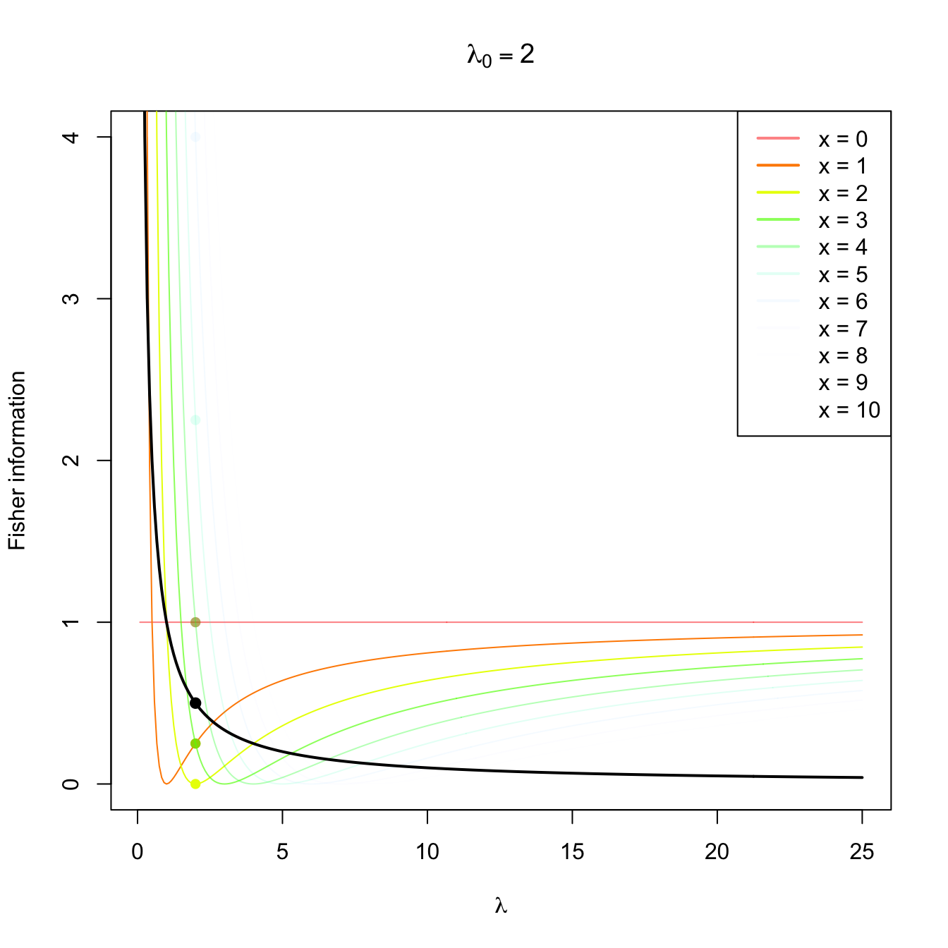
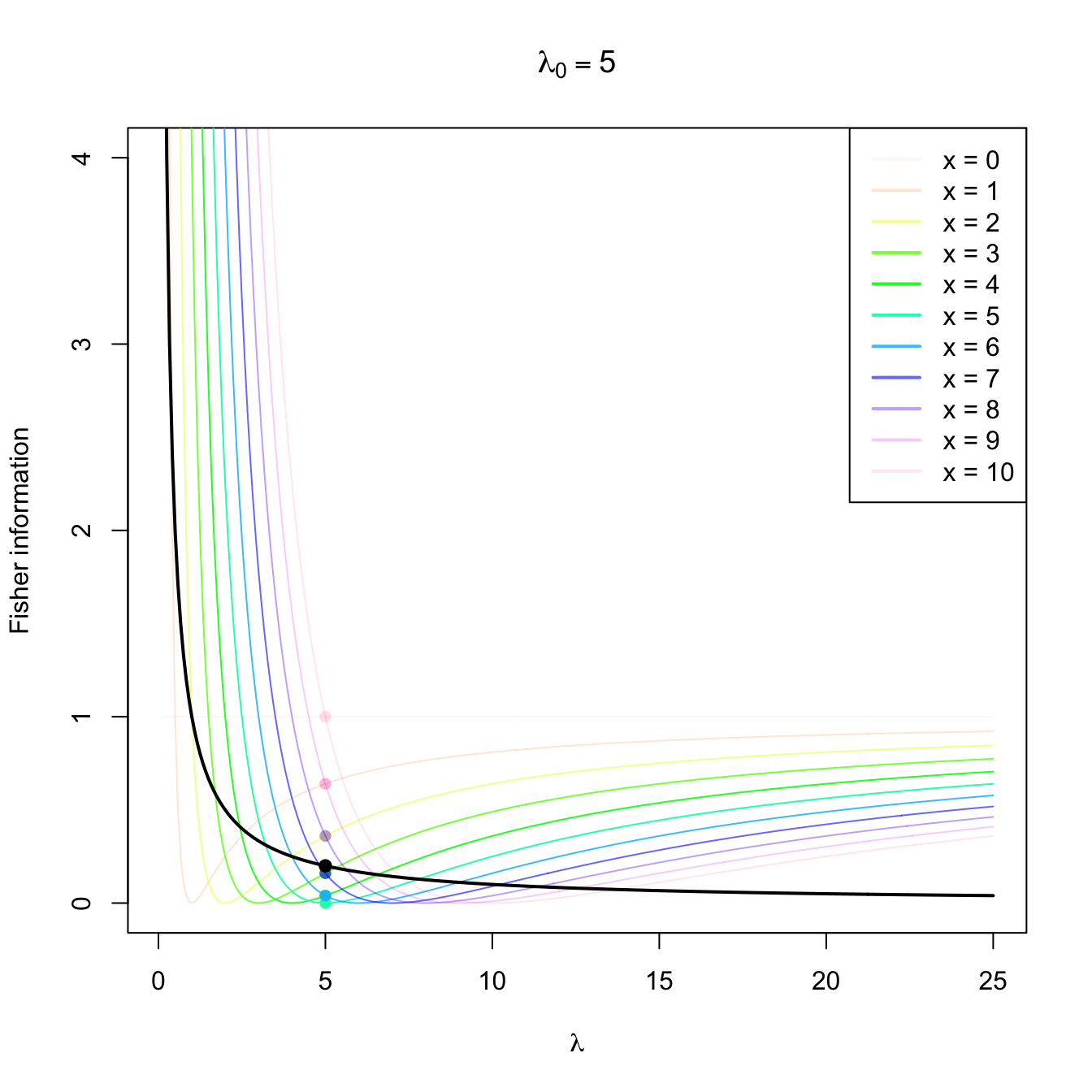
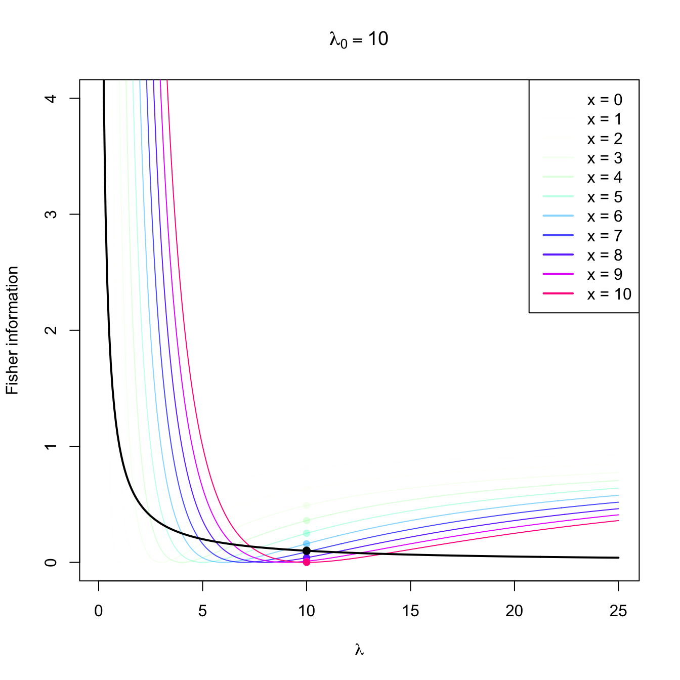
Figure 3.4: Fisher information integrand \(\lambda\mapsto \left(\partial \log f(x;\lambda)/\partial \lambda\right)^2\) in a \(\mathrm{Pois}(\lambda_0)\) distribution with \(\lambda_0=2,5,10.\) The integrands are shown in different colors, with the color transparency indicating the probability of \(x\) according to \(\mathrm{Pois}(\lambda_0)\) (the darker the color, the higher the probability). The Fisher information curve \(\lambda\mapsto \mathcal{I}(\lambda)\) is shown in black, with a black point signaling the value \(\mathcal{I}(\lambda_0).\) The colored points indicate the contribution of each \(x\) to the Fisher information.

When taking the expectation in (3.7), we obtain that the Fisher information is the expected information of \(X\) that is useful to distinguish \(\theta\) from close values. This quantity is related with the precision (i.e., the inverse of the variance) of an unbiased estimator of \(\theta.\)

Example 3.30 Compute the Fisher’s information of a rv \(X\sim \mathrm{Pois}(\lambda).\)

The Poisson’s pmf is given by

\[\begin{align*} p(x;\lambda)=\frac{\lambda^x e^{-\lambda}}{x!}, \quad x=0,1,2,\ldots, \end{align*}\]

so its logarithm is

\[\begin{align*} \log{p(x;\lambda)}=x\log{\lambda}-\lambda-\log{(x!)} \end{align*}\]

and its derivative with respect to \(\lambda\) is

\[\begin{align*} \frac{\partial \log p(x;\lambda)}{\partial \lambda}=\frac{x}{\lambda}-1. \end{align*}\]

The Fisher information is then obtained taking the expectation of³⁹

\[\begin{align*} \left(\frac{\partial \log p(X;\lambda)}{\partial \lambda}\right)^2=\left(\frac{X-\lambda}{\lambda}\right)^2, \end{align*}\]

Noting that \(\mathbb{E}[X]=\lambda\) and, therefore, \(\mathbb{E}[(X-\lambda)^2]=\mathbb{V}\mathrm{ar}[X]=\lambda,\) we obtain

\[\begin{align} \mathcal{I}(\lambda)=\mathbb{E}\left[\left(\frac{X-\lambda}{\lambda}\right)^2\right]=\frac{\mathbb{V}\mathrm{ar}[X]}{\lambda^2}=\frac{1}{\lambda}.\tag{3.9} \end{align}\]

The following fundamental result states the lower variance bound of an unbiased estimator that is regular enough. Hence, it establishes the lowest MSE that an unbiased estimator can attain and thus establishes a reference for other unbiased estimators. The inequality is also known as the information inequality.

Theorem 3.8 (Crámer–Rao’s inequality) Let \((X_1,\ldots,X_n)\) be a srs of a rv with pdf \(f(x;\theta),\) and let \[\begin{align*} \mathcal{I}_n(\theta):=n\mathcal{I}(\theta) \end{align*}\] be the Fisher’s information of the sample \((X_1,\ldots,X_n)\) about \(\theta.\) If \(\hat{\theta}\equiv\hat{\theta}(X_1,\ldots,X_n)\) is an unbiased estimator of \(\theta\) then, under certain general conditions,⁴⁰ it holds

\[\begin{align*} \mathbb{V}\mathrm{ar}\big[\hat{\theta}\big]\geq \frac{1}{\mathcal{I}_n(\theta)}. \end{align*}\]

Definition 3.13 (Efficient estimator) An unbiased estimator \(\hat{\theta}\) of \(\theta\) that verifies \(\mathbb{V}\mathrm{ar}\big[\hat{\theta}\big]=(\mathcal{I}_n(\theta))^{-1}\) is said to be efficient.

Example 3.31 Show that for a rv \(\mathrm{Pois}(\lambda)\) the estimator \(\hat{\lambda}=\bar{X}\) is efficient.

We first calculate the Fisher information \(\mathcal{I}_n(\theta)\) of the sample \((X_1,\ldots,X_n).\) Since \(\mathcal{I}(\lambda)=1/\lambda\) from Example 3.30, then

\[\begin{align*} \mathcal{I}_n(\lambda)&=n\mathcal{I}(\lambda)=\frac{n}{\lambda}. \end{align*}\]

On the other hand, the variance of \(\hat{\lambda}=\bar{X}\) is

\[\begin{align*} \mathbb{V}\mathrm{ar}[\hat{\lambda}]=\frac{1}{n^2}\mathbb{V}\mathrm{ar}\left[\sum_{i=1}^n X_i\right]=\frac{n\lambda}{n^2}=\frac{\lambda}{n}. \end{align*}\]

Therefore, \(\hat{\lambda}=\bar{X}\) is efficient.

Example 3.32 Check that \(\hat{\theta}=\bar{X}\) is efficient for estimating \(\theta\) in a population \(\mathrm{Exp}(1/\theta).\)

3.7 Robust estimators

An estimator \(\hat{\theta}\) of the parameter \(\theta\) associated to a rv with pdf \(f(\cdot;\theta)\) is robust if it preserves good properties (small bias and variance) even if the model suffers from small contamination, that is, if the assumed density \(f(\cdot;\theta)\) is just an approximation of the true density due to the presence of observations coming from other distributions.

The theory of statistical robustness is deep and has a broad toolbox of methods aimed for different contexts. This section just provides some ideas for robust estimation of the mean \(\mu\) and the standard deviation \(\sigma\) of a population. For that, we consider the following widely-used contamination model for \(f(\cdot;\theta)\):

\[\begin{align*} f(x;\theta,\varepsilon,g):=(1-\varepsilon)f(x;\theta)+\varepsilon g(x), \quad x\in \mathbb{R}, \end{align*}\]

for a small \(0<\varepsilon<0.5\) and an arbitrary pdf \(g.\) The model features a mixture of the signal pdf, \(f(\cdot;\theta),\) and the contamination pdf, \(g.\) The percentage of contamination is \(100\varepsilon\%.\)

The first example shows that the sample mean is not robust for this kind of contamination.

Example 3.33 (\(\bar{X}\) is not robust for \(\mu\)) Let \(f(\cdot;\theta)\) be the pdf of a \(\mathcal{N}(\theta,\sigma^2)\) and \((X_1,\ldots,X_n)\) a srs of that distribution. In absence of contamination, we know that the variance of the sample mean is \(\mathbb{V}\mathrm{ar}_\theta(\bar{X})=\sigma^2/n.\) It is an efficient estimator (Exercise 3.22). However, if we now contaminate with the pdf \(g\) of a \(\mathcal{N}(\theta, c\sigma^2),\) where \(c>0\) is a constant, then the variance of the sample mean \(\bar{X}\) under \(f(x;\theta,\varepsilon,c)\) becomes

\[\begin{align*} \mathbb{V}\mathrm{ar}_{\theta,\varepsilon,c}(\bar{X})=(1-\varepsilon)\sigma^2/n+\varepsilon c^2\sigma^2/n=(\sigma^2/n)(1+\varepsilon [c^2-1]). \end{align*}\]

Therefore, the relative variance increment under contamination is

\[\begin{align*} \frac{\mathbb{V}\mathrm{ar}_{\theta,\varepsilon,c}(\bar{X})}{\mathbb{V}\mathrm{ar}_\theta(\bar{X})}=1+\varepsilon [c^2-1]. \end{align*}\]

For \(c=5\) and \(\varepsilon=0.01,\) the ratio is \(1.24.\) In addition, \(\lim_{c\to\infty} \mathbb{V}\mathrm{ar}_{\theta,\varepsilon,c}(\bar{X})=\infty,\) for all \(\varepsilon>0.\) Therefore, \(\bar{X}\) is not robust.

The concept of outlier is intimately related with robustness. Outliers are “abnormal” observations in the sample that seem very unlikely for the assumed distribution model or are remarkably different from the rest of sample observations.⁴¹ Outliers can be originated by measurement errors, exceptional circumstances, changes in the data generating process, etc.

There are two main approaches for preventing outliers or contamination to undermine the estimation of \(\theta\):

1. Detect the outliers through a diagnosis of the model fit and re-estimate the model once the outliers have been removed.
2. Employ a robust estimator.

The first approach is the traditional one and is still popular due to its simplicity. Besides, it allows using non-robust efficient estimators that tend to be simpler to compute, provided the data has been cleared adequately. However, robust estimators may be needed even when performing the first approach, as the following example illustrates.

A simple rule to detect outliers in a normal population is to flag as outliers the observations that lie further away than \(3\sigma\) from the mean \(\mu,\) since those observations are highly extreme. Since their probability is \(0.0027,\) we expect to flag as an outlier \(1\) out of \(371\) observations if the data comes from a perfectly normal population. However, applying this procedure entails estimating first \(\mu\) and \(\sigma\) from the data. But the conventional estimators, the sample mean and variance, are also very sensitive to outliers, and therefore their estimates may hide the existence of outliers. Therefore, it is better to rely on a robust estimator, which brings us back to the second approach.

The next definition introduces a simple measure of the robustness of an estimator.

Definition 3.14 (Finite-sample breakdown point) For a sample realization \(\boldsymbol{x}=(x_1,\ldots,x_n)^\top\) and an integer \(m\) with \(1\leq m\leq n,\) define the set of samples that differ from \(\boldsymbol{x}\) in \(m\) observations as

\[\begin{align*} U_m({\boldsymbol{x}}):=\{\boldsymbol{y}=(y_1,\ldots,y_n)^\top\in\mathbb{R}^n : |\{i: x_i\neq y_i\}|=m\}. \end{align*}\]

The maximum change of an estimator \(\hat{\theta}\) when \(m\) observations are contaminated is

\[\begin{align*} A(\boldsymbol{x},m):=\sup_{\boldsymbol{y}\in U_m({\boldsymbol{x}})} |\hat{\theta}(\boldsymbol{y})-\hat{\theta}(\boldsymbol{x})| \end{align*}\]

and the breakdown point of \(\hat{\theta}\) for \(\boldsymbol{x}\) is

\[\begin{align*} \max\left\{\frac{m}{n}:A(\boldsymbol{x},m)<\infty\right\}. \end{align*}\]

The breakdown point of an estimator \(\hat{\theta}\) can be interpreted as the maximum fraction of the sample that can be changed without modifying the value of \(\hat{\theta}\) to an arbitrarily large value.

Example 3.34 It can be seen that:

• The breakdown point of the sample mean is \(0.\)
• The breakdown point of the sample median is \(\lfloor n/2\rfloor/n,\) with \(\lfloor n/2\rfloor/n\to0.5\) as \(n\to\infty.\)
• The breakdown point of the sample variance (and of the standard deviation) is \(0.\)

The so-called trimmed means defined below form a popular class of robust estimators for \(\mu\) that generalizes the mean (and median) in a very intuitive way.

Definition 3.15 (Trimmed mean) Let \((X_1,\ldots, X_n)\) be a sample. The \(\alpha\)-trimmed mean at level \(0\leq \alpha\leq 0.5\) is defined as

\[\begin{align*} T_{\alpha}:=\frac{1}{n-2m(\alpha)}\sum_{i=m(\alpha)+1}^{n-m(\alpha)}X_{(i)} \end{align*}\]

where \(m(\alpha):=\lfloor n\cdot \alpha\rfloor\) is the number of trimmed observations at each extreme and \((X_{(1)},\ldots, X_{(n)})\) is the ordered sample such that \(X_{(1)}\leq\cdots\leq X_{(n)}.\)

Observe that \(\alpha=0\) corresponds to the sample mean and \(\alpha=0.5\) to the sample median. The next result reveals that the breakdown point of the trimmed mean is approximately equal to \(\alpha>0,\) which is larger than that of the sample mean. Of course, this gain in robustness is at the expense of a moderate loss of efficiency in the form of an increased variance, which in a normal population is about a \(6\%\) increment when \(\alpha=0.10.\)

Proposition 3.1 (Properties of the trimmed mean)

1. For symmetric distributions, \(T_{\alpha}\) is unbiased for \(\mu.\)
2. The breakdown point of \(T_{\alpha}\) is \(m(\alpha)/n,\) with \(m(\alpha)/n\to\alpha\) as \(n\to\infty.\)
3. For \(X\sim \mathcal{N}(\mu,\sigma^2),\) \(\mathbb{V}\mathrm{ar}(T_{0.1})\approx1.06\cdot \sigma^2/n\) for large \(n.\)

Another well-known class of robust estimators for the population mean is the class of \(M\)-estimators.

Definition 3.16 (\(M\)-estimator for \(\mu\)) An \(M\)-estimator for \(\mu\) based on the sample \((X_1,\ldots,X_n)\) is a statistic

\[\begin{align} \tilde{\mu}:=\arg \min_{m\in\mathbb{R}} \sum_{i=1}^n \rho\left(\frac{X_i-m}{\hat{s}}\right),\tag{3.10} \end{align}\]

where \(\hat{s}\) is a robust estimator of the standard deviation (such that \(\tilde{\mu}\) is scale-invariant) and \(\rho\) is the objective function, which satisfies the following properties:

1. \(\rho\) is nonnegative: \(\rho(x)\geq 0,\) \(\forall x\in\mathbb{R}.\)
2. \(\rho(0)=0.\)
3. \(\rho\) is symmetric: \(\rho(x)=\rho(-x),\) \(\forall x\in\mathbb{R}.\)
4. \(\rho\) is monotone nondecreasing: \(x\leq x'\implies \rho(x)\leq \rho(x'),\) \(\forall x,x'\in\mathbb{R}.\)

Example 3.35 The sample mean is the least squares estimator of the mean, that is, it minimizes

\[\begin{align*} \bar{X}=\arg\min_{m\in\mathbb{R}} \sum_{i=1}^n (X_i-m)^2 \end{align*}\]

and therefore is an \(M\)-estimator with \(\rho(x)=x^2.\)

Analogously, the sample median minimizes the sum of absolute distances

\[\begin{align*} \arg\min_{m\in\mathbb{R}} \sum_{i=1}^n |X_i-m| \end{align*}\]

and hence is an \(M\)-estimator with \(\rho(x)=|x|.\)

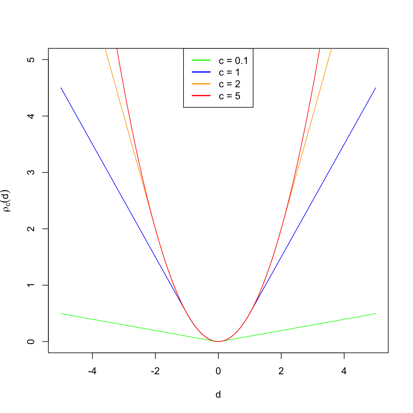
Figure 3.5: Huber’s rho function for different values of \(c\).

A popular objective function is Huber’s rho function:

\[\begin{align*} \rho_c(d)=\begin{cases} 0.5d^2 & \text{if} \ |d| \leq c,\\ c |d|-0.5c^2 & \text{if} \ |d|>c, \end{cases} \end{align*}\]

for a constant \(c>0.\) For small distances, \(\rho_c\) employs quadratic distances, as in the case of the sample mean. For large distances (that are more influential), it employs absolute distances, as the sample median does. Therefore, setting \(c\to\infty\) yields the sample mean in (3.10) and using \(c\to0\) gives the median. As with trimmed means, we therefore have an interpolation between mean (non-robust) and median (robust) that is controlled by one parameter.

Finally, a robust alternative for estimating \(\sigma\) is the median absolute deviation.

Definition 3.17 (Median absolute deviation) The Median Absolute Deviation (MAD) of a sample \((X_1,\ldots,X_n)\) is defined as

\[\begin{align*} \text{MAD}(X_1,\ldots,X_n):=c\cdot \mathrm{med}\{|X_1-\mathrm{med}\{X_1,\ldots,X_n\}|,\ldots,|X_n-\mathrm{med}\{X_1,\ldots,X_n\}| \}, \end{align*}\]

where \(\mathrm{med}\{X_1,\ldots,X_n\}\) stands for the median of the sample and \(c\) corrects the MAD such that it is centered for \(\sigma\) in normal populations:

\[\begin{align*} \mathbb{P}(|X-\mu| \le \sigma/c)=0.5\iff c=1/\Phi(0.75)\approx 1.48. \end{align*}\]

Appendix

Useful probability inequalities

The following two probability inequalities are useful to show consistency in probability.

Proposition 3.2 (Markov's inequality) For any rv \(X,\)

\[\begin{align*} \mathbb{P}(|X| \geq k)\leq \frac{\mathbb{E}[X^2]}{k^2}, \quad k> 0. \end{align*}\]

Proof (Proof of Proposition 3.2). Assume that \(X\) is a continuous rv and let \(f\) be its pdf. We compute the second-order moment of \(X\):

\[\begin{align*} \mathbb{E}[X^2] &=\int_{-\infty}^{\infty} x^2 f(x)\,\mathrm{d}x\\ &=\int_{(-\infty,-k]\cup[k,\infty)} x^2 f(x)\,\mathrm{d}x+\int_{(-k,k)} x^2 f(x)\,\mathrm{d}x \\ &\geq\int_{(-\infty,-k]\cup[k,\infty)} x^2 f(x)\,\mathrm{d}x \\ &\geq k^2 \int_{(-\infty,-k]\cup[k,\infty)} f(x)\,\mathrm{d}x\\ &=k^2\mathbb{P}(|X| \geq k), \end{align*}\]

which is equivalent to

\[\begin{align*} \mathbb{P}(|X| \geq k)\leq \frac{\mathbb{E}[X^2]}{k^2}. \end{align*}\]

The proof for a discrete rv is analogous.

Proposition 3.3 (Chebyshev's inequality) Let \(X\) a rv with \(\mathbb{E}[X]=\mu\) and \(\mathbb{V}\mathrm{ar}[X]=\sigma^2<\infty.\) Then,

\[\begin{align*} \mathbb{P}\left(|X-\mu| \geq k\sigma\right)\leq \frac{1}{k^2}, \quad k>0. \end{align*}\]

Proof (Proof of Proposition 3.3). This inequality follows from Markov’s inequality. Indeed, taking

\[\begin{align*} X'=X-\mu, \quad k'=k\sigma, \end{align*}\]

and replacing \(X\) by \(X'\) and \(k\) by \(k'\) in Markov’s inequality, we get

\[\begin{align*} \mathbb{P}(|X-\mu| \geq k\sigma)\leq\frac{\sigma^2}{k^2\sigma^2}=\frac{1}{k^2}. \end{align*}\]

Chebyshev’s inequality is useful for obtaining probability bounds about \(\hat{\theta}\) when its probability distribution is unknown. We only need to know the expectation and variance of \(\hat{\theta}.\) Indeed, taking \(k=2,\) the Chebyshev’s inequality gives

\[\begin{align*} \mathbb{P}\big(|\hat{\theta}-\theta| \leq 2\sigma_{\hat{\theta}}\big)\geq 1-\frac{1}{4}=0.75, \end{align*}\]

which means that at least the \(75\%\) of the realized values of \(\hat{\theta}\) fall within the interval \([\theta-2\sigma_{\hat{\theta}},\theta+2\sigma_{\hat{\theta}}].\) However, if we additionally know that the distribution of the estimator \(\hat{\theta}\) is normal, \(\hat{\theta}\sim\mathcal{N}(\theta,\sigma_{\hat{\theta}}^2),\) then we obtain the much more precise result

\[\begin{align*} \mathbb{P}\big(|\hat{\theta}-\theta| \leq 2\sigma_{\hat{\theta}}\big)\approx 0.95>0.75. \end{align*}\]

The fact that the true probability, \(\approx 0.95,\) is in this case substantially larger than the lower bound given by Chebyshev’s inequality, \(0.75,\) is reasonable: Chebyshev’s inequality does not employ any knowledge on the distribution of \(\hat{\theta}.\) Thus, the precision increases as there is more information about the true distribution of \(\hat{\theta}.\)

Example 3.36 From previous experience, it is known that the time \(X\) (in minutes) that a periodic check of a machine requires is distributed as \(\Gamma(3,2).\) A new worker spends \(19\) minutes checking that machine. Is this time coherent with the previous experience?

We know that the mean and the variance of a gamma are given by

\[\begin{align*} \mu=\alpha\beta=3\times 2=6,\quad\sigma^2=\alpha\beta^2=3\times 2^2=12\to\sigma\approx 3.46. \end{align*}\]

Then, the difference between the checking time of the new worker and \(\mu\) is \(19-6=13.\) To see whether this difference is large or small, or, in other words, to see whether the checking time of this new worker is in line with previous checking times, we would want to know the probability

\[\begin{align*} \mathbb{P}(|X-\mu| \geq 13). \end{align*}\]

For that, we take \(k\sigma=13\) in Chebyshev’s inequality, so \(k=13/\sigma=13/3.46=3.76,\) and applying the inequality we readily get

\[\begin{align*} \mathbb{P}(|X-\mu| \geq 13)\leq \frac{1}{k^2}=\frac{1}{3.76^2}=0.071. \end{align*}\]

Since this probability bound is very small, the checking time is not coherent with the previous experience. Two things may have happened: either the new worker has faced a more complicated inspection or he/she is slower than the rest.

Rao–Blackwell’s Theorem

Rao–Blackwell’s Theorem provides an effective form of reducing the variance of an unbiased estimator using a sufficient statistic \(T.\) This process is sometimes known as Rao–Blackwellization and results in a new estimator with lower MSE.

Theorem 3.9 (Rao–Blackwell’s Theorem) Let \(T\) be a sufficient statistic for \(\theta.\) Let \(\hat{\theta}\) be an unbiased estimator of \(\theta.\) Then, the estimator

\[\begin{align*} \hat{\theta}':=\mathbb{E}\big[\hat{\theta} \mid T\big] \end{align*}\]

verifies:

1. \(\hat{\theta}'\) is independent of \(\theta.\)
2. \(\mathbb{E}\big[\hat{\theta}'\big]=\theta,\) \(\forall \theta\in \Theta.\)
3. \(\mathbb{V}\mathrm{ar}\big[\hat{\theta}'\big]\leq \mathbb{V}\mathrm{ar}\big[\hat{\theta}\big],\) \(\forall\theta\in\Theta.\)

In addition, \(\mathbb{V}\mathrm{ar}\big[\hat{\theta}'\big]= \mathbb{V}\mathrm{ar}\big[\hat{\theta}\big]\) if and only if \(\mathbb{P}\big(\hat{\theta}'=\hat{\theta}\big)=1,\) \(\forall \theta \in \Theta.\)

Observe that the new estimator \(\hat{\theta}'\) depends on the sample through the sufficient statistic \(T\) and, in particular, on the minimal sufficient statistic.

Example 3.37 Let \((X_1,\ldots,X_n)\) be a srs of \(X\sim \mathrm{Pois}(\lambda),\) that is, with pmf

\[\begin{align*} p(x;\lambda)=\frac{\lambda^x e^{-\lambda}}{x!}, \quad x=0,1,\ldots, \ \lambda>0. \end{align*}\]

Consider the parameter \(\theta=p(0;\lambda)=e^{-\lambda}.\) Let us perform a Rao–Blackwellization.

First, we need an unbiased estimator, for example:

\[\begin{align*} \hat{\theta}=\begin{cases} 1 & \text{if} \ X_1=0,\\ 0 & \text{if} \ X_1\neq 0, \end{cases} \end{align*}\]

since

\[\begin{align*} \mathbb{E}\big[\hat{\theta}\big]=1\times\mathbb{P}(X_1=0)+ 0\times\mathbb{P}(X_1\neq 0)=\mathbb{P}(X_1=0)=e^{-\lambda}. \end{align*}\]

Now we need a sufficient estimator. Writing the pmf of the Poisson in the form of the exponential family, we obtain

\[\begin{align*} p(x;\lambda)=e^{-\lambda}\frac{e^{x\log{\lambda}}}{x!} \end{align*}\]

and therefore \(T(X_1,\ldots,X_n)=\sum_{i=1}^n X_i\) is sufficient for \(\lambda\) and also for \(e^{-\lambda}.\)

Then, we can Rao–Blackwellize \(\hat{\theta}\):

\[\begin{align*} \hat{\theta}':=&\;\mathbb{E}\big[\hat{\theta} \mid T\big]\\ =&\;1\times\mathbb{P}\left(X_1=0\Bigg| \sum_{i=1}^n X_i=t\right)+0\times\mathbb{P}\left(X_1\neq 0\Bigg| \sum_{i=1}^n X_i=t\right) \\ =&\;\frac{\mathbb{P}(X_1=0,\sum_{i=1}^n X_i=t)}{\mathbb{P}(\sum_{i=1}^n X_i=t)}\\ =&\;\frac{\mathbb{P}(X_1=0)\mathbb{P}(\sum_{i=2}^n X_i=t)}{\mathbb{P}(\sum_{i=1}^n X_i=t)}. \end{align*}\]

Now, it holds that, if \(X_i\sim \mathrm{Pois}(\lambda),\) \(i=1,\ldots,n,\) are independent, then (see Exercise 1.20)

\[\begin{align*} \sum_{i=1}^n X_i \sim \mathrm{Pois}(n\lambda). \end{align*}\]

Therefore,

\[\begin{align*} \hat{\theta}'=\frac{e^{-\lambda}[(n-1)\lambda]^t e^{-(n-1)\lambda}/t!}{(n\lambda)^t e^{-n\lambda}/t!}=\left(\frac{n-1}{n}\right)^t. \end{align*}\]

Then, we have obtained the estimator

\[\begin{align*} \hat{\theta}'=\mathbb{E}\big[\hat{\theta} \mid T\big]=\left(\frac{n-1}{n}\right)^T, \end{align*}\]

which is unbiased, and whose variance is smaller than the one of \(\hat{\theta}.\) Indeed,

\[\begin{align*} \mathbb{E}\big[\hat{\theta}'\big]&=\sum_{x=1}^{\infty} \left(\frac{n-1}{n}\right)^x \frac{e^{-n\lambda}(n\lambda)^x}{x!}\\ &=e^{-n\lambda}\sum_{x=0}^{\infty} \frac{(n-1)^x \lambda^x}{x!}\\ &=e^{-n\lambda}e^{(n-1)\lambda}\\ &=e^{-\lambda}=\theta. \end{align*}\]

Therefore, \(\hat{\theta}'\) is unbiased. We compute its variance. For that, in the first place, we compute

\[\begin{align*} \mathbb{E}\big[\hat{\theta}'^2\big] &=\sum_{t=0}^{\infty}\left(\frac{n-1}{n}\right)^{2t} \frac{e^{-n\lambda}(n\lambda)}{t!}\\ &=e^{-n\lambda}\sum_{t=0}^{\infty}\left(\frac{(n-1)^2\lambda}{n}\right)\frac{1}{t!} \\ &=e^{-n\lambda}e^{(n-1)^2\lambda/n}\\ &=e^{-2\lambda+\lambda/n}. \end{align*}\]

Then, the variance is

\[\begin{align*} \mathbb{V}\mathrm{ar}\big[\hat{\theta}'\big]=\mathbb{E}\big[\hat{\theta}'^2\big]-\mathbb{E}^2\big[\hat{\theta}'\big]=e^{-2\lambda+\lambda/n}-e^{-2\lambda}=e^{-2\lambda}(e^{\lambda/n}-1). \end{align*}\]

We calculate the variance of \(\hat{\theta}\) for comparison:

\[\begin{align*} \mathbb{E}\big[\hat{\theta}^2\big]=1\times\mathbb{P}(X_1=0)=e^{-\lambda}. \end{align*}\]

As a consequence,

\[\begin{align*} \mathbb{V}\mathrm{ar}\big[\hat{\theta}\big]=e^{-\lambda}-e^{-2\lambda}=e^{-\lambda}(1-e^{-\lambda}). \end{align*}\]

Therefore,

\[\begin{align*} \frac{\mathbb{V}\mathrm{ar}\big[\hat{\theta}'\big]}{\mathbb{V}\mathrm{ar}\big[\hat{\theta}\big]}=\frac{e^{-2\lambda}(e^{\lambda/n}-1)}{e^{-\lambda}(1-e^{-\lambda})}=\frac{e^{\lambda/n}-1}{e^{\lambda}-1}<1, \quad \forall n\geq 1. \end{align*}\]

Exercises

Exercise 3.1 We have a srs of size \(n\) from a population with mean \(\mu\) and variance \(\sigma^2.\)

1. Prove that \(\sum_{i=1}^na_iX_i\) is an unbiased estimator of \(\mu\) if \(\sum_{i=1}^na_i=1.\)
2. Among all the unbiased estimators of this form, find the one with minimum variance and compute it.

Exercise 3.2 Let \((X_1,\ldots,X_n)\) be a srs from a \(\mathcal{U}\left(0, \theta \right),\) \(\theta >0.\) Find out whether the following estimators are unbiased for the population mean and, in case of a positive answer, find their biases:

\[\begin{align*} \bar{X},\quad X_1,\quad X_{(n)},\quad X_{(1)},\quad 0.5 X_{(n)}+0.5 X_{(1)}. \end{align*}\]

Exercise 3.3 The consumption of a certain good in a family with four members during the summer months is a rv with \(\mathcal{U}(\alpha,\alpha+1)\) distribution. Let \((X_1,\ldots,X_n)\) be a srs of consumption of the same good for different families.

1. Show that the sample mean is biased for \(\alpha\) and that its bias is \(1/2.\)
2. Compute the MSE of \(\bar{X}\) as an estimator of \(\alpha.\)
3. Obtain from \(\bar{X}\) an unbiased estimator of \(\alpha\) and provide its MSE.

Exercise 3.4 Let \((X_1,\ldots,X_n)\) be a srs from an \(\mathrm{Exp}(\lambda).\)

1. Find an unbiased estimator of \(\lambda\) based on \(X_{(1)}.\)
2. Compare the previous estimator with \(\bar{X}\) and decide which one is better.
3. The lifetime of a light bulb in days is usually modeled by an exponential distribution. The following data are lifetimes for light bulbs: \(50.1,\) \(70.1,\) \(137,\) \(166.9,\) \(170.5,\) \(152.8,\) \(80.5,\) \(123.5,\) \(112.6,\) \(148.5,\) \(160,\) \(125.4.\) Estimate the average duration of a light bulb using the two previous estimators.

Exercise 3.5 Assume that the rv’s \(Y_1,\ldots,Y_n\) are such that

\[\begin{align*} Y_i=\beta x_i+\varepsilon_i,\quad i=1,\ldots,n, \end{align*}\]

where the \(x_i\)’s are constants and the \(\varepsilon_i\) are iid rv’s distributed as \(\mathcal{N}(0,\sigma^2).\)

1. Prove that \(\sum_{i=1}^nY_i/\sum_{i=1}^nx_i\) is an unbiased estimator of \(\beta.\)
2. Prove that \((1/n)\sum_{i=1}^nY_i/x_i\) is also unbiased.
3. Compute the variances of both estimators.

Exercise 3.6 Let \((X_1,\ldots,X_{n_1})\) be a srs of \(X\) with \(\mathbb{E}[X]=\mu_1\) and \(\mathbb{V}\mathrm{ar}[X]=\sigma^2,\) and let \((Y_1,\ldots ,Y_{n_2})\) be a srs of \(Y\) with \(\mathbb{E}[Y]=\mu_2\) and \(\mathbb{V}\mathrm{ar}[Y]=\sigma^2,\) with \(X\) and \(Y\) independent.

1. Prove that \(S^2:=wS_1'^2+(1-w)S_2'^2\) is a consistent estimator of \(\sigma^2,\) for any \(w\in(0,1).\)
2. Show that

\[\begin{align*} \frac{\bar{X}-\bar{Y}-(\mu_1-\mu_2)}{S\sqrt{{\frac{1}{n_1}}+{\frac{1}{n_2}}}}\stackrel{d}{\longrightarrow} \mathcal{N}(0,1). \end{align*}\]

Exercise 3.7 The number of independent arrivals to an emergency service during a day follows a \(\mathrm{Pois}(\lambda)\) distribution. In order to estimate \(\lambda\) and forecast the amount of required personnel in the service, we observe the arrivals during \(n\) days. We know that \(T=\sum_{i=1}^nX_i\) is a sufficient statistic. Determine:

1. \(k>0\) such that the estimator \(T_k=kT\) is unbiased for \(\lambda.\)
2. The condition that the sequence \(k_n\) must satisfy for obtaining a sequence of estimators that is consistent in probability, if the sample size \(n\) is allowed to grow.

Exercise 3.8 Consider a sample as in Exercise 3.2.

1. Prove that \(X_{(n)}\) is consistent in probability for \(\theta.\)
2. Check whether \(Y_n=2\bar{X}_n\) is also consistent in probability for \(\theta.\)

Exercise 3.9 Let \((X_1,\ldots,X_{10})\) be a srs from a distribution with mean \(\mu\) and variance \(\sigma^2.\) Consider the following two estimators of \(\mu\):

\[\begin{align*} \hat{\mu}_1=X_1+\frac{1}{2}X_2-\frac{1}{2}X_3, \quad \hat{\mu}_2=X_4+\frac{1}{5}X_5-\frac{1}{10}X_{10}. \end{align*}\]

Which one is better in terms of MSE? Are they consistent in probability?

Exercise 3.10 Let \((X_1,\ldots,X_n)\) be a srs from a distribution with mean \(\mu\) and variance \(\sigma^2.\) Consider the following estimators of \(\mu\):

\[\begin{align*} \hat{\mu}_1=\frac{X_1+2X_2+3X_3}{6}, \quad \hat{\mu}_2=\frac{X_1+4X_2+X_3}{6}, \quad \hat{\mu}_3=\frac{\frac{3}{2}X_1+\frac{1}{2}X_2+X_3+\cdots+X_n}{n}. \end{align*}\]

1. Which ones are unbiased?
2. Among the unbiased ones, which is the most efficient?
3. Find an unbiased estimator of \(\mu\) different from \(\bar{X}\) that is more efficient than the previous unbiased estimators.
4. Which of them is consistent in squared mean?

Exercise 3.11 Let \((X_1,\ldots,X_n)\) be a srs of a rv with \(\mathrm{Pois}(\lambda)\) distribution. Check that

\[\begin{align*} \frac{\bar{X}-\lambda}{\sqrt{\bar{X}/n}}\stackrel{d}{\longrightarrow}\mathcal{N}(0,1). \end{align*}\]

Exercise 3.12 Prove the law of the large numbers from Theorem 3.2 using Theorem 3.1.

Exercise 3.13 Let \((X_1,\ldots,X_n)\) be a srs from a geometric distribution, whose pmf is

\[\begin{align*} p(x;\theta) =\theta (1-\theta)^{x-1},\quad x=1,2,\ldots,\ \theta \in (0, 1). \end{align*}\]

Prove that \(\sum_{i=1}^nX_i\) is sufficient for \(\theta.\)

Exercise 3.14 Let \((X_1,\ldots,X_n)\) be a srs from a population with pdf

\[\begin{align*} f(x;\theta)=\frac{2x}{\theta}e^{-x^2/\theta} 1_{\{x>0\}},\quad \theta>0. \end{align*}\]

Show that \(\sum_{i=1}^n X_i^2\) is sufficient for \(\theta\) and that \(\sum_{i=1}^n X_i\) is not.

Exercise 3.15 Let \((X_1,\ldots,X_n)\) be a srs from a continuous Bernoulli distribution, whose pdf is

\[\begin{align*} f(x;\lambda) = c(\lambda) \lambda^x(1-\lambda)^{1-x},\quad x\in[0,1],\ \lambda \in (0,1), \end{align*}\]

with \(c(\lambda)=21_{\{\lambda=1/2\}}+ \frac{2 \tanh^{-1}(1-2 \lambda)}{1-2 \lambda}1_{\{\lambda\neq 1/2\}}.\) Find a sufficient statistic for \(\lambda.\)

Exercise 3.16 Let \(X_1\) be a normal rv with mean zero and variance \(\sigma^2.\) Is \(|X_1|\) a sufficient statistic for \(\sigma^2\)?

Exercise 3.17 Let \((X_1,\ldots,X_n)\) be a srs from a particular Weibull distribution with pdf

\[\begin{align*} f(x;\theta)=\frac{2x}{\theta}e^{-x^2/\theta}, \quad x>0,\ \theta>0. \end{align*}\]

Find a minimal sufficient statistic for \(\theta.\)

Exercise 3.18 Let \((X_1,\ldots,X_n)\) be a srs from a Laplace distribution \(\mathrm{Laplace}(\mu,\sigma),\) whose pdf is

\[\begin{align*} f(x;\mu,\sigma)=\frac{1}{2\sigma}e^{-|x-\mu|/\sigma}, \quad x\in\mathbb{R},\ \mu\in\mathbb{R},\ \sigma>0. \end{align*}\]

Find a minimal sufficient statistic for \(\sigma\) assuming that \(\mu\) is known.

Exercise 3.19 Let \((X_1,\ldots,X_n)\) be a srs from a beta distribution \(\mathrm{Beta}(\alpha,\beta),\) whose pdf is

\[\begin{align*} f(x;\alpha,\beta)=\frac{\Gamma(\alpha+\beta)}{\Gamma(\alpha) \Gamma(\beta)} x^{\alpha-1}(1-x)^{\beta-1}, \quad x\in(0,1),\ \alpha>0,\ \beta>0. \end{align*}\]

Find a minimal sufficient statistic for:

1. \(\alpha,\) assuming that \(\beta\) is known.
2. \(\beta,\) assuming that \(\alpha\) is known.

Exercise 3.20 Compute the Fisher information for \(X\sim\mathrm{Exp}(\lambda).\) Then, derive an efficient estimator for \(\lambda.\)

Exercise 3.21 Is it possible to compute the Fisher information for the following distributions?

1. \(\mathcal{U}(0,\theta).\)
2. The pdf \(f(x;\theta)=\theta/x^2,\) \(x\geq\theta>0.\)

What do these two distributions have in common?

Exercise 3.22 Let \((X_1,\ldots,X_n)\) be a srs of a rv \(X\sim\mathcal{N}(\mu,\sigma^2).\) Show that \(\bar{X}\) is an efficient estimator of \(\mu.\)

Exercise 3.23 Let \((X_1,\ldots,X_{n_1})\) be a srs of \(X\sim \mathcal{N}(\mu_1,\sigma^2)\) and let \((Y_1,\ldots,Y_{n_2})\) be a srs of \(Y\sim \mathcal{N}(\mu_2,\sigma^2),\) with \(X\) and \(Y\) independent. As an estimator of \(\sigma^2,\) we consider a linear combination of the sample quasivariances \(S_1'^2\) and \(S_2'^2,\) that is, \(w S_1'^2 + (1-w)S_2'^2,\) for \(0\leq w \leq 1.\)

1. Prove that this estimator is unbiased for any value of \(w.\)
2. Obtain the value of \(w\) that provides the most efficient estimator.

Exercise 3.24 Consider a srs \((X_1,\ldots,X_n)\) from a \(\mathrm{Cauchy}(\theta,\sigma)\) distribution. Use a simulation like that in Figure 3.1 to check empirically if \(\hat{\theta}_n\) is a consistent estimator for \(\theta.\) Consider these estimators:

1. \(\hat{\theta}_n=\bar{X}.\)
2. \(\hat{\theta}_n=\mathrm{med}\{X_1,\ldots,X_n\}.\)
3. \(\hat{\theta}_n=T_{0.10}\) (\(0.10\)-trimmed mean).

Explore in each case \(N=5\) simulations for each of the three choices of \((\theta,\sigma)\) and a sequence of \(n\)’s that increase at least until \(n=10^4.\) What are your conclusions?

Exercise 3.25 The Fisher information (3.7) is an expectation. Therefore, from a srs \((X_1,\ldots,X_n)\) from a continuous rv with pdf \(f(\cdot;\theta),\) it can be approximated as the sample mean

\[\begin{align*} \hat{\mathcal{I}}(\theta):=\frac{1}{n}\sum_{i=1}^n \left(\frac{\partial \log f(X_i;\theta)}{\partial \theta}\right)^2. \end{align*}\]

The construction is analogous for a discrete rv.

Consider a \(\mathrm{Pois}(\lambda)\) distribution. Use a simulation to check empirically how \(\hat{\mathcal{I}}(\lambda)\) approximates \(\mathcal{I}(\lambda)=1/\lambda\) by:

1. Plotting the curve \(\lambda\mapsto\mathcal{I}(\lambda)\) over the grid lambda <- seq(1, 10, by = 0.5).
2. For each lambda, simulating \((X_1,\ldots,X_n)\sim\mathrm{Pois}(\lambda)\) and plotting the curve \(\lambda\mapsto\hat{\mathcal{I}}(\lambda).\)

Use \(n=10,100,1000.\) What are your conclusions? What if in Step 2 the simulation was done from \((X_1,\ldots,X_n)\sim\mathrm{Pois}(\lambda_0),\) \(\lambda_0=2,\) for each lambda?

References

Lehmann, E. L., and G. Casella. 1998. Theory of Point Estimation. Second. Springer Texts in Statistics. New York: Springer-Verlag. https://doi.org/10.1007/b98854.

---

32. Can you think of a class of transformations for which unbiasedness is actually preserved?↩︎

33. Note that Definition 3.5 is a particular case of Definition 3.6 with \(X\) being a degenerate random variable that takes the value \(\theta\) with probability one.↩︎

34. We expanded the square inside the MSE, as opposed to use the bias–variance decomposition, to rely on previous computations for \(\mathbb{E}\big[\hat{\theta}_n\big].\)↩︎

35. To actually show that \(\hat{\mu}_1\) is not consistent in probability, observe that \(\mathbb{P}(|\hat{\mu}_1-\mu|>\varepsilon)\) does not depend on \(n.\) For \(\hat{\mu}_2,\) use that \(\hat{\mu}_2\stackrel{\mathbb{P}}{\longrightarrow} \frac{X_1+X_2}{4}+\frac{\mu}{2}\) due to Theorem 3.2 and Corollary 3.3.↩︎

36. If there is no dependence on \(\theta,\) neither it is on \(g(\theta).\)↩︎

37. Note that \(\{X_1=x_1,\ldots,X_n=x_n\}=\{X_1=x_1,\ldots,X_n=x_n\} \cap\{T=t\}\) because \(t=T(x_1,\ldots,x_n).\) The intersection does not impose a restriction, but it is useful to make it explicit.↩︎

38. In a non-injective mapping, \(\varphi(x)=\varphi(y)\) does not imply that \(x=y.\) There might be different elements \(x\) and \(y\) having the same image by \(\varphi.\)↩︎

39. Note that we change \(x\) to \(X\) because now we have to work with a random variable to take an expectation.↩︎

40. See Theorem 5.10 (Section 2.5, page 120) in Lehmann and Casella (1998).↩︎

41. The concept of outlier is subjective, although there are several mathematical definitions of outliers.↩︎