6 Hypothesis tests

Figure 6.1: Power curve of the one-sided hypothesis test for \(H_0:\sigma^2=\sigma_0^2\) vs. \(H_1:\sigma^2>\sigma_0^2\) in a normal population \(\mathcal{N}(0,\sigma^2).\) The power curve represents the probability of rejecting \(H_0:\sigma^2=\sigma_0^2,\) as a function of \(\sigma,\) from a sample of size \(n\) from \(\mathcal{N}(0,\sigma^2).\) The dashed vertical line is the value of \(\sigma_0=1\) and the dotted horizontal line is the significance level \(\alpha=0.10.\) The power increases as \(n\) increases and as \(\sigma\) increases, as the evidence against \(H_0:\sigma^2=\sigma_0^2\) is stronger in those cases. Observe how a one-sided test has no power when \(\sigma^2<\sigma_0^2,\) since it is designed to “face” \(H_1:\sigma^2>\sigma_0^2\).

Hypothesis tests are arguably the main tool in statistical inference to answer research questions in a precise and formal way that takes into account the uncertainty behind the data generation and measurement process. This chapter introduces the basics of hypothesis testing, the best-known tests for one and two normal populations, and the theory of likelihood ratio tests.

6.1 Introduction

The following example serves to illustrate the main philosophy in hypothesis testing.

Example 6.1 A pharmaceutical company suspects that a given drug in testing produces an increment of the ocular tension as a secondary effect. The basis tension level has mean \(15\) and the suspected increment is towards a mean of \(18\) units. This increment may increase the risk of suffering glaucoma. Since the drug has a positive primary effect, it is important to check if this suspicion is true before moving forward on the commercialization of the drug.

Medical trials have established that, at a population level, the ocular tension tends to follow a \(\mathcal{N}(15,1)\) distribution. The suspicion about the secondary effect then means that the ocular tension among the takers of the drug would be \(\mathcal{N}(18,1).\) We denote by \(X\sim\mathcal{N}(\mu,1)\) the rv “ocular tension of the takers of the drug”. Then, the question the pharmaceutical company faces is to decide whether \(\mu=15\) (the drug has no secondary effect) or \(\mu=18\) (the drug has a secondary effect) based on empirical evidence. To formalize this, we define:

\[\begin{align*} \begin{cases} H_0:\mu=15 & \text{(null hypothesis)} \\ H_1:\mu=18 & \text{(alternative hypothesis)} \end{cases} \end{align*}\]

Then, we want to find evidence in favor of \(H_0\) or of \(H_1.\) But, since the drug has been proven effective, the pharmaceutical company is only willing to stop its commercialization if there is enough evidence against \(H_0\) (or in favor of \(H_1\)), that is, if there is enough evidence pointing to the presence of a secondary effect. Therefore, the roles of \(H_0\) and \(H_1\) are not symmetric. \(H_0\) is a “stickier” belief than \(H_1\) for the pharmaceutical company.

In order to look for evidence against \(H_0\) or in favor of \(H_1,\) a sample of the ocular tension level of four drug takers is measured, and its sample mean \(\bar{X}\) is computed. Then, the following is verified:

• If \(H_0\) is true, then \(\bar{X}\sim \mathcal{N}(15,1/4).\)
• If \(H_1\) is true, then \(\bar{X}\sim \mathcal{N}(18,1/4).\)

Then, if we obtain a small value of \(\bar{X},\) we will have little or no evidence in favor of \(H_1\) and believe \(H_0.\) If we obtain a large value of \(\bar{X},\) then the sample supports \(H_1.\) But, up to which value of \(\bar{X}=k_1\) are we willing to believe in \(H_0\)?

This question can be answered in the following way: we can limit the possibility of incorrectly stopping the commercialization of the drug to a small value \(\alpha,\) i.e.,

\[\begin{align*} \mathbb{P}(\text{Reject $H_0$} \mid \text{$H_0$ true})\leq \alpha, \end{align*}\]

and choose the constant \(k_1\) that satisfies this, that is, choose the smallest \(k_1\) that verifies

\[\begin{align*} \mathbb{P}(\text{Reject $H_0$} \mid \text{$H_0$ true})=\mathbb{P}(\bar{X}>k_1 \mid \mu=15)\leq \alpha. \end{align*}\]

Standardizing \(\bar{X},\) we obtain the standard normal distribution. Then \(k_1\) directly follows from the quantiles of such a distribution:

\[\begin{align*} \mathbb{P}(\bar{X}> k_1 \mid \mu=15)=\mathbb{P}(2(\bar{X}-15)> 2(k_1-15))=\mathbb{P}(Z> 2(k_1-15))\leq \alpha. \end{align*}\]

From here, we have that \(2(k_1-15)=z_{\alpha},\) so \(k_1=15+z_{\alpha}/2.\) For example, if we take \(\alpha=0.05,\) then \(z_{\alpha}\approx1.645\) and \(k_1\approx15+1.645/2=15.8225.\) Therefore, if we obtain \(\bar{X}>15.8225\) and \(H_0\) was true, the obtained sample would belong to this “extreme” set that only has probability \(\alpha=0.05.\) This implies that one of the following two possibilities is happening if the event \(\{\bar{X}>k_1\}\) happens:

1. either \(H_0\) is true but the obtained sample was “extreme” and is not very representative of its distribution;
2. or \(H_0\) is not true because an event with low probability if \(H_0\) was true just happened.

Following the logic of believing \(H_0\) or not based on how likely is the realization of \(\bar{X}\) under the assumption of truth of \(H_0,\) a rule to make a decision on the veracity of \(H_0\) is the following:

• “Reject \(H_0\)” if \(\bar{X}>k_1,\) as it is unlikely that the event \(\{\bar{X}>k_1\}\) happened if \(H_0\) is true;
• “Do not reject \(H_0\)” if \(\bar{X}\leq k_1,\) as it is likely that the event \(\{\bar{X}\leq k_1\}\) happened if \(H_0\) is true.

The level \(\alpha\) determines the probability of the data-dependent extreme event that is inconsistent with the veracity of \(H_0\) and that triggers its rejection. A choice of \(\alpha=0.05\) by the pharmaceutical company implies that the drug commercialization will only be stopped if the outcome of the ocular tension level test is only \(5\%\) likely under the assumption that the drug has no secondary effect.

Example 6.2 We could make the same reasoning that we have made in Example 6.1, now with respect to \(H_1.\) For small values of \(\bar{X},\) we would think that \(H_1\) is not true. But, up to which value \(\bar{X}=k_2\) are we willing to believe \(H_1\)?

If we fix again a bound for the probability of committing an error (in this case, allowing the commercialization of the drug while it has secondary effects), \(\beta,\) that is,

\[\begin{align*} \mathbb{P}(\text{Reject $H_1$} \mid \text{$H_1$ true})\leq \beta, \end{align*}\]

then we will choose the larger constant \(k_2\) that verifies that relation, that is, that verifies

\[\begin{align*} \mathbb{P}(\text{Reject $H_1$} \mid \text{$H_1$ true})=\mathbb{P}(\bar{X}\leq k_2 \mid \mu=18)\leq \beta. \end{align*}\]

Standardizing \(\bar{X}\) in the previous probability, we obtain

\[\begin{align*} \mathbb{P}(\bar{X}\leq k_2 \mid \mu=18)&=\mathbb{P}(2(\bar{X}-18)\leq 2(k_2-18) \mid \mu=18)\\ &=\mathbb{P}(Z\leq 2(k_2-18))\leq \beta, \end{align*}\]

in such a way that \(2(k_2-18)=-z_{\beta},\) so \(k_2=18-z_{\beta}/2.\) Taking \(\beta=0.05,\) we have \(z_{\beta}\approx1.645,\) and \(k_2\approx18-1.645/2=17.1775.\)

Then, following this argument and combining this with the reasoning for \(H_0\) in Example 6.1, the decision would be:

• If \(\bar{X}\leq k_1\approx 15.8225,\) then we accept \(H_0.\)
• If \(\bar{X}\geq k_2\approx 17.1775,\) then we accept \(H_1.\)

The following question arises immediately: what shall we do if \(15.8225<\bar{X}<17.1775\)? Also, imagine that instead of \(15\) units, the basis ocular tension level was \(16.5\) units. Then \(16.5+1.645/2=17.3225>k_2\) and we will be accepting \(H_0\) and \(H_1\) at the same time! These inconsistencies point towards focusing on choosing just a single value \(k\) from which to make a decision. But in this case, only one of the probabilities for the two types of error, \(\alpha\) and \(\beta,\) can be controlled.

If we decrease \(\alpha\) too much, \(\beta\) will increase. In addition, it may happen that \(\bar{X}>k,\) so we would not have evidence against \(H_0,\) but that the sample is neither representative of \(H_1.\) It may also happen that \(\bar{X}\leq k,\) so we will not have evidence against \(H_0,\) but that however the sample is more representative of \(H_1\) than of \(H_0.\) Therefore, if we want to control \(\alpha,\) in the first place we have to fix the null hypothesis \(H_0\) as the most conservative statement, that is, the statement that will be assumed as true unless there is enough evidence against it. As a consequence, the decision to be made is going to be one of the following:

• “Reject \(H_0\)” if \(\bar{X}>k_1\) (without commitment to accept \(H_1\));
• “Do not reject \(H_0\)” if \(\bar{X}\leq k_1\) (without commitment to reject \(H_1,\) which could be valid).

In general, through this section we assume a rv \(X\) with distribution within the family of distributions \(\{F(\cdot;\theta):\theta\in\Theta\}\) for which we want to determine the validity of a statement \(H_0\) about the parameter \(\theta\) against an alternative statement \(H_1.\) Splitting the parametric space as \(\Theta=\Theta_0\cup\Theta_1\cup\Theta_2,\) where typically⁷⁴ \(\Theta_1=\bar{\Theta}_0\) and \(\Theta_2=\emptyset,\) the hypotheses to test are of the form

\[\begin{align*} H_0:\theta\in\Theta_0 \quad \text{vs.}\quad H_1:\theta\in\Theta_1. \end{align*}\]

Recall that a statement about the unknown parameter \(\theta\) is equivalent to a statement about the distribution \(F(\cdot;\theta).\)

Definition 6.1 (Null and alternative hypotheses) The null hypothesis (denoted by \(H_0\)) is the statement that is assumed true unless there is enough evidence against it. The confronting statement is the alternative hypothesis (denoted by \(H_1\)).

Definition 6.2 (Simple and composite hypotheses) If the set \(\Theta_0\subset \Theta\) that determines the hypothesis \(H_0\) contains a single element,⁷⁵ then \(H_0\) is said to be a simple hypothesis. Otherwise, \(H_0\) is referred to as a composite hypothesis.

The decision in favor of or against \(H_0\) is made from the information available in the realization of a srs \((X_1,\ldots,X_n)\) of \(X.\)

Definition 6.3 (Test) A test or a hypothesis test of \(H_0\) vs. \(H_1\) is a function \(\varphi:\mathbb{R}^n\to\{0,1\},\) where \(1\) stands for “reject \(H_0\) in favor of \(H_1\)” and \(0\) for “do not reject \(H_0\)”, of the form

\[\begin{align*} \varphi(x_1,\ldots,x_n)=\begin{cases} 1 & \text{if}\ (x_1,\ldots,x_n)^\top\in C,\\ 0 & \text{if}\ (x_1,\ldots,x_n)^\top\in \bar{C}, \end{cases} \end{align*}\]

where \(C\) and \(\bar{C}\) provide a partition of the sample space \(\mathbb{R}^n.\) The set \(C\) is denoted as the critical region or rejection region and \(\bar{C}\) is the acceptance region.

A hypothesis test is entirely determined by the critical region \(C.\) In principle, there exist infinitely many tests for testing a hypothesis at hand. The selection of a particular test is done according to the test reliability, that is, according to its “success rate”. The possible consequences — with respect to the reality about \(H_0,\) which is unknown — of a test decision are given in the following table:

Test decision \(\backslash\) Reality	\(H_0\) true	\(H_0\) false
Do not reject \(H_0\)	Correct decision	Type II error
Reject \(H_0\)	Type I error	Correct decision

Then, the reliability of a hypothesis test is quantified and assessed in terms of the two possible types of errors:

Error	Interpretation
Type I error	Reject \(H_0\) if it is true
Type II error	Do not reject \(H_0\) if it is false

As illustrated in Examples 6.1 and 6.2, the classical procedure for selecting a test among all the available ones is the following:

1. Fix a bound, \(\alpha,\) for the probability of committing the Type I error. This bound is the significance level of the hypothesis test.

2. Exclude all the tests with critical regions \(C\) that do not respect the bound for the Type I error, that is, that do not satisfy the condition \[\begin{align*} \mathbb{P}(\text{Reject $H_0$} \mid H_0\ \text{true})=\mathbb{P}((X_1,\ldots,X_n)^\top\in C \mid \text{$H_0$ true})\leq \alpha. \end{align*}\]

3. Among the selected tests, choose the one that has a critical region \(C\) that minimizes the Type II error, that is, that minimizes \[\begin{align*} \beta=\mathbb{P}(\text{Do not reject $H_0$} \mid \text{$H_1$ true})=\mathbb{P}((X_1,\ldots,X_n)^\top\in \bar{C} \mid H_1 \ \text{true}). \end{align*}\]

Instead of determining the critical region \(C\) directly as a subset of \(\mathbb{R}^n,\) it is simpler to determine it through a statistic of the sample and express the critical region as a subset of the range of a statistic. Then, a test statistic will determine the rejection region of the test.

Definition 6.4 (Test statistic) A test statistic of a hypothesis \(H_0\) vs. \(H_1\) is a measurable function of the sample that involves \(H_0\) and under \(H_0\) has a known or approximable distribution.

A test statistic can be obtained usually by taking an estimator of the unknown parameter that is involved in \(H_0\) and transforming it in such a way that it has a usable distribution under \(H_0.\)

Summarizing what has been presented until now, the key elements of a hypothesis test are:

• a null hypothesis \(H_0\) and an alternative \(H_1;\)
• a significance level \(\alpha;\)
• a test statistic;
• and a critical region \(C.\)

The following practical takeaways are implied by the definitions of \(H_0\) and \(H_1\) and are relevant for deciding how to assign \(H_0\) and \(H_1\) when carrying out a hypothesis test.

When deciding between how to assign a research question to \(H_0\) or \(H_1\) in a real application, remember:

• \(H_1\) is used for the statement that the researcher is “interested” in proving through the sample.
• \(H_0\) is the de facto statement that is assumed true unless there is enough evidence against it in the sample. It cannot be proved using a hypothesis test – at most it is not rejected (but not accepted either).

If we are interested in testing the veracity of “Statement”, it is stronger to

1. reject \(H_0: \overline{\mathrm{Statement}}\) in favor of \(H_1: \mathrm{Statement}\) than
2. do not reject \(H_0: \mathrm{Statement}\) vs. \(H_1: \overline{\mathrm{Statement}}.\)

In the first case we do find evidence in favor of “Statement”; in the second case we do not find evidence against “Statement”. Above, \(\overline{\mathrm{Statement}}\) is the negation of \(\mathrm{Statement}.\)

Example 6.3 A political poll is made in order to know the voting intentions of the electorate regarding two candidates, A and B, and, specifically, if candidate A will win the elections. For that purpose, the number of voters \(Y\) who will vote for candidate A within a sample of \(n=15\) voters was recorded. The associated hypothesis test for this problem is

\[\begin{align*} H_0:p=0.5\quad \text{vs.}\quad H_1:p>0.5, \end{align*}\]

where \(p\) denotes the proportion of voters in favor of \(A.\) If \(Y\) is the test statistic and the rejection region is set as \(C=\{y\geq 12\},\) compute the probability of the Type I error for the test, \(\alpha.\)

The probability of the Type I error is

\[\begin{align*} \alpha=\mathbb{P}(\text{Type error I})=\mathbb{P}(\text{Reject $H_0$} \mid \text{$H_0$ true})=\mathbb{P}(Y\geq 12 \mid p=0.5). \end{align*}\]

Since \(Y\sim \mathrm{Bin}(n,0.5),\) the previous probability is

\[\begin{align*} \alpha=\sum_{y=12}^{15} \binom{15}{y}(0.5)^{15}\approx0.0176. \end{align*}\]

Example 6.4 Assume that the real proportion of voters for the candidate A is \(p=0.6\) (so \(H_0\) is false). What is the probability that in the test of Example 6.3 we obtain that candidate A will not win (\(H_0\) is not rejected)?

The probability of Type II error is

\[\begin{align*} \beta=\mathbb{P}(\text{Type error II})=\mathbb{P}(\text{Do not reject $H_0$} \mid \text{$H_0$ false}). \end{align*}\]

In this case, we want to compute the value of \(\beta\) for \(p=0.6,\) that is,

\[\begin{align*} \beta&=\mathbb{P}(Y<12 \mid p=0.6)=\sum_{y=0}^{11} \binom{15}{y}(0.6)^y(0.4)^{15-y}\approx0.9095. \end{align*}\]

Then, if we employ that rejection region, the test would most likely conclude that candidate A will win, whether the candidate is actually going to win or not. The test is conservative due to the small sample size \(n\) and \(\alpha=0.0176.\)⁷⁶

6.2 Tests on a normal population

We assume in this section that the population rv \(X\) has distribution \(\mathcal{N}(\mu,\sigma^2),\) where both \(\mu\) and \(\sigma^2\) are unknown. We will test hypotheses about one of the two parameters from a srs \((X_1,\ldots,X_n)\) of \(X.\) The sampling distributions obtained in Section 2.2 are key for obtaining the critical regions of the forthcoming tests.

6.2.1 Tests about the mean

6.2.1.1 One-sided right test

We want to test the hypothesis⁷⁷

\[\begin{align*} H_0:\mu=\mu_0 \quad \text{vs.}\quad H_1:\mu > \mu_0. \end{align*}\]

As seen in the previous section, we must fix first the bound \(\alpha\) for the probability of Type I error, that is,

\[\begin{align} \mathbb{P}(\text{Reject $H_0$} \mid \text{$H_0$ true})\leq \alpha.\tag{6.1} \end{align}\]

To obtain the critical region, we need a statistic \(T(X_1,\ldots,X_n).\) If we take \(\bar{X},\) whose distribution is \(\mathcal{N}(\mu_0,\sigma^2/n),\) then we should reject the null hypothesis for large values of \(\bar{X}.\) Therefore, the critical region has the form

\[\begin{align*} C=\{(x_1,\ldots,x_n)^\top\in \mathbb{R}^n: \bar{X}>k\}, \end{align*}\]

for a given value \(k.\) We can compute the constant \(k\) in such a way that verifies (6.1), that is, such that

\[\begin{align} \mathbb{P}(\bar{X}>k \mid \mu=\mu_0)\leq \alpha.\tag{6.2} \end{align}\]

But there are infinitely many values \(k\) that satisfy the above relation. For example, if we consider a value \(k_1\) that is not the smallest one, then there will be another value \(k_2<k_1\) such that

\[\begin{align*} \mathbb{P}(\bar{X}>k_1 \mid \mu=\mu_0)\leq \mathbb{P}(\bar{X}>k_2 \mid \mu=\mu_0)\leq \alpha. \end{align*}\]

Then, it will happen that the probability of Type II error of the test with critical region \(\{\bar{X}>k_1\}\) will be larger than the one for the test with critical region \(\{\bar{X}>k_2\}.\) Therefore, among the tests with critical region of the type \(\{\bar{X}>k\}\) that verify (6.2), the most efficient is the one with smallest \(k.\)

However, recall that in this case it is not possible to determine the smallest \(k\) that verifies (6.2) since the distribution of \(\bar{X}\) is partially unknown (\(\sigma^2\) is unknown). But if we estimate \(\sigma^2\) with \(S'^2,\) then a test statistic is

\[\begin{align} T(X_1,\ldots,X_n)=\frac{\bar{X}-\mu_0}{S'/\sqrt{n}}\stackrel{H_0}{\sim} t_{n-1}.\tag{6.3} \end{align}\]

Determining the critical region from \(T\) is simple, since the range of \(T\) is \(\mathbb{R}\) and therefore the critical region is an interval of \(\mathbb{R}.\) The null hypothesis is to be rejected for large values of \(T,\) hence the critical region is of the form \(\{T(x_1,\ldots,x_n)>k\}.\) We must select the smallest \(k\) such that

\[\begin{align*} \mathbb{P}(T>k \mid \mu=\mu_0)\leq \alpha. \end{align*}\]

From here, it is deduced that \(k=t_{n-1;\alpha}.\) Therefore, the critical region is

\[\begin{align*} C &=\{(x_1,\ldots,x_n)^\top\in\mathbb{R}^n: T(x_1,\ldots,x_n)>t_{n-1;\alpha}\} \\ &=\left\{(x_1,\ldots,x_n)^\top\in\mathbb{R}^n: \frac{\bar{X}-\mu_0}{S'/\sqrt{n}}>t_{n-1;\alpha} \right\} \\ &=\left\{(x_1,\ldots,x_n)^\top\in\mathbb{R}^n: \bar{X}>\mu_0+t_{n-1;\alpha}\frac{S'}{\sqrt{n}}\right\}. \end{align*}\]

Observe that the quantity \(t_{n-1;\alpha}\frac{S'}{\sqrt{n}}\) can be regarded as the “uncertainty tolerance” that is added to the no-uncertainty rule that would reject \(H_0:\mu=\mu_0\) if \(\bar{X}>\mu_0.\)

6.2.1.2 One-sided left test

If the null hypothesis to test is

\[\begin{align*} H_0:\mu=\mu_0 \quad \text{vs.}\quad H_1:\mu < \mu_0, \end{align*}\]

then the test statistic is exactly the same as before, but in this case we must reject the null hypothesis for small values of \(T.\) Therefore, the critical region has the form \(\{T<k\}.\) Fixing a significance level \(\alpha\) and selecting the larger \(k\) that verifies the relation

\[\begin{align*} \mathbb{P}(T<k \mid \mu=\mu_0)\leq \alpha \end{align*}\]

we get that the value of \(k\) is \(k=-t_{n-1;\alpha}\) and the critical region is

\[\begin{align*} C=\{(x_1,\ldots,x_n)^\top\in\mathbb{R}^n : T(x_1,\ldots,x_n)<-t_{n-1;\alpha}\}. \end{align*}\]

6.2.1.3 Two-sided test

Now we want to test the hypothesis

\[\begin{align*} H_0:\mu=\mu_0 \quad \text{vs.}\quad H_1:\mu\neq \mu_0. \end{align*}\]

For the same test statistic (6.3), now we will reject for large absolute values of \(T\) that will indicate deviation from \(H_0.\) That is, the critical region has the form

\[\begin{align*} \{(x_1,\ldots,x_n)^\top\in\mathbb{R}^n: T(x_1,\ldots,x_n)\in(-\infty,k_1)\cup (k_2,\infty)\}. \end{align*}\]

Now we must determine the value of the two constants \(k_1\) and \(k_2\) in such a way that

\[\begin{align*} \mathbb{P}(T\in(-\infty,k_1)\cup (k_2,\infty) \mid \mu=\mu_0)\leq \alpha. \end{align*}\]

Evenly splitting \(\alpha/2\) to both tails, since the distribution of \(T\) under \(H_0\) is \(t_{n-1}\) and is symmetric, gives \(k_2=t_{n-1;\alpha/2}\) and \(k_1=-t_{n-1;\alpha/2}.\) Then, the critical region is

\[\begin{align*} C=\{(x_1,\ldots,x_n)^\top\in\mathbb{R}^n : |T(x_1,\ldots,x_n)|>t_{n-1;\alpha/2}\}. \end{align*}\]

Example 6.5 Eight bullets made of a new type of gunpowder were fired in a gun, and their initial speeds in m/s were measured:

\[\begin{align*} 910,\quad 921,\quad 918,\quad 896,\quad 909,\quad 905,\quad 895,\quad 903. \end{align*}\]

The producer of the gunpowder claims that the new gunpowder delivers an average initial speed above \(915\) m/s. Is the sample providing evidence against such claim, at the significance level \(\alpha=0.025\)? Assume that the initial speeds follow a normal distribution.

We want to test the hypothesis

\[\begin{align*} H_0:\mu=915\quad \text{vs.}\quad H_1:\mu<915. \end{align*}\]

The critical region is

\[\begin{align*} C=\{T<-t_{7;0.025}\approx-2.365\}. \end{align*}\]

The observed value of the statistic is

\[\begin{align*} T=\frac{\bar{X}-\mu_0}{S'/\sqrt{n}}\approx\frac{907.125-915}{9.3723/\sqrt{8}}\approx -2.377<-2.365. \end{align*}\]

Then, the observed initial speeds are sufficiently low to question the claim of the gunpowder producer.

Recall that \(t_{7;0.025}\) can be computed as

qt(0.025, df = 7, lower.tail = FALSE)
## [1] 2.364624

The R function t.test() implements the (one-sample) test of \(H_0:\mu=\mu_0\) against different alternatives. The main arguments of the function are as follows:

t.test(x, alternative = c("two.sided", "less", "greater"), mu = 0, ...)

The argument mu stands for \(\mu_0.\) The table below shows the encoding of the alternative argument:

alternative	"two.sided"	"less"	"greater"
\(H_1\)	\(\mu\neq\mu_0\)	\(\mu<\mu_0\)	\(\mu>\mu_0\)

Example 6.6 The t.test() solution to Example 6.5 is very simple:

# Apply t.test() with H1: mu < 915
t.test(x = c(910, 921, 918, 896, 909, 905, 895, 903), mu = 915,
       alternative = "less")
## 
##  One Sample t-test
## 
## data:  c(910, 921, 918, 896, 909, 905, 895, 903)
## t = -2.3766, df = 7, p-value = 0.02456
## alternative hypothesis: true mean is less than 915
## 95 percent confidence interval:
##      -Inf 913.4029
## sample estimates:
## mean of x 
##   907.125

That the reported \(p\)-value is smaller than \(\alpha=0.025\) indicates rejection of \(H_0,\) as seen in Section 6.5.

6.2.2 Tests about the variance

We study in this section the tests for the following hypotheses:

1. \(H_0:\sigma^2=\sigma_0^2\) vs. \(H_1:\sigma^2>\sigma_0^2;\)
2. \(H_0:\sigma^2=\sigma_0^2\) vs. \(H_1:\sigma^2<\sigma_0^2;\)
3. \(H_0:\sigma^2=\sigma_0^2\) vs. \(H_1:\sigma^2\neq\sigma_0^2.\)

An estimator of \(\sigma^2\) is the sample quasivariance, \(S'^2,\) for which we perfectly know its distribution under the null hypothesis,

\[\begin{align*} U=\frac{(n-1)S'^2}{\sigma_0^2}\stackrel{H_0}\sim \chi_{n-1}^2. \end{align*}\]

Therefore, \(U\) is a test statistic for the testing problems a, b, and c.

When testing case a, if the null hypothesis is not true, \(U\) will tend to have large values. Therefore, the critical region is of the form \(\{U>k\}.\) For obtaining the best value \(k,\) we select the significance level \(\alpha\) and take the smallest \(k\) such that

\[\begin{align*} \mathbb{P}(U>k \mid \sigma^2=\sigma_0^2)\leq \alpha. \end{align*}\]

Then, the best choice is \(k=\chi_{n-1;\alpha}^2,\) so the critical region is

\[\begin{align*} C_a=\{(x_1,\ldots,x_n)^\top\in\mathbb{R}^n:U(x_1,\ldots,x_n)>\chi_{n-1;\alpha}^2\}. \end{align*}\]

With an analogous reasoning, the critical region for b follows:

\[\begin{align*} C_b=\{(x_1,\ldots,x_n)^\top\in\mathbb{R}^n:U(x_1,\ldots,x_n)<\chi_{n-1;1-\alpha}^2\}. \end{align*}\]

The critical region for c arises from splitting evenly the probability \(\alpha\) in the critical regions of a and b:

\[\begin{align*} C_c=\{(x_1,\ldots,x_n)^\top\in\mathbb{R}^n:U(x_1,\ldots,x_n)>\chi_{n-1;\alpha/2}^2 \ \text{or}\ U(x_1,\ldots,x_n)<\chi_{n-1;1-\alpha/2}^2\}. \end{align*}\]

Example 6.7 A company claims that the diameter of one of the parts of an engine it produces has a production variance not larger than \(0.1290\) squared millimeters. A srs of \(10\) pieces revealed \(S'^2=0.1935.\) Assuming that the measurements of the diameter follow a normal distribution, test at a significance level \(\alpha=0.05\)

\[\begin{align*} H_0:\sigma^2=0.1290\quad \text{vs.} \quad H_1:\sigma^2>0.1290. \end{align*}\]

The test statistic is

\[\begin{align*} U=\frac{(n-1)S'^2}{\sigma_0^2}=\frac{9\times 0.1935}{0.1290}=13.5 \end{align*}\]

and the rejection region is

\[\begin{align*} C=\{U>\chi_{9;0.05}^2\approx16.919\}. \end{align*}\]

Since \(U=13.5<16.919,\) then the data does not provide any evidence against the variance of the diameter being larger than \(0.1290\) squared millimeters. Therefore, there is no evidence against the company’s claim.

Unfortunately, there is no function in base R to conduct the (one-sample) variance test.

6.3 Tests on two normal populations

We assume now two populations represented as two independent rv’s \(X_1\sim\mathcal{N}(\mu_1,\sigma_1^2)\) and \(X_2\sim\mathcal{N}(\mu_2,\sigma_2^2),\) with unknown means and variances. From two srs’s \((X_{11},\ldots,X_{1n_1})\) and \((X_{21},\ldots,X_{2n_2})\) of \(X_1\) and \(X_2,\) we will test hypotheses about the difference of means \(\mu_1-\mu_2,\) assuming \(\sigma_1^2=\sigma_2^2,\) and about the ratio of variances \(\sigma_1^2/\sigma_2^2.\) As in Section 6.2, the sampling distributions obtained in Section 2.2 for normal populations will be key for obtaining the critical regions of the forthcoming tests.

6.3.1 Equality of means

We assume that \(\sigma_1^2=\sigma_2^2=\sigma^2.\) The hypotheses to test are of three types:

1. \(H_0:\mu_1=\mu_2\) vs. \(H_1:\mu_1>\mu_2;\)
2. \(H_0:\mu_1=\mu_2\) vs. \(H_1:\mu_1<\mu_2;\)
3. \(H_0:\mu_1=\mu_2\) vs. \(H_1:\mu_1\neq \mu_2.\)

Denoting \(\theta:=\mu_1-\mu_2,\) then the hypotheses can be rewritten as:

1. \(H_0:\theta=0\) vs. \(H_1:\theta>0;\)
2. \(H_0:\theta=0\) vs. \(H_1:\theta<0;\)
3. \(H_0:\theta=0\) vs. \(H_1:\theta\neq 0.\)

An estimator of \(\theta\) is the difference of sample means,

\[\begin{align*} \hat{\theta}=\bar{X}_1-\bar{X}_2\sim \mathcal{N}\left(\mu_1-\mu_2,\sigma^2\left(\frac{1}{n_1}+\frac{1}{n_2}\right)\right). \end{align*}\]

If we estimate \(\sigma^2\) using

\[\begin{align*} S^2=\frac{(n_1-1)S_1'^2+(n_2-1)S_2'^2}{n_1+n_2-2}, \end{align*}\]

then an adequate test statistic is

\[\begin{align*} T=\frac{\bar{X}_1-\bar{X}_2}{S\sqrt{\frac{1}{n_1}+\frac{1}{n_2}}}\stackrel{H_0}\sim t_{n_1+n_2-2}. \end{align*}\]

It does not take much to realize that the critical regions can be completely recycled from that in Section 6.2.1. Therefore, the critical regions are:

1. \(C_a=\{T>t_{n_1+n_2-2;\alpha}\};\)
2. \(C_b=\{T<-t_{n_1+n_2-2;\alpha}\};\)
3. \(C_c=\{|T|>t_{n_1+n_2-2;\alpha/2}\}.\)

Example 6.8 Is there any evidence that any of the two training methods described in Example 5.5 works better with \(\alpha=0.05\)? The average assembly times for the two groups of nine employees were \(\bar{X}_1\approx35.22\) and \(\bar{X}_2\approx31.56,\) and the quasivariances \(S_1'^2\approx24.445\) and \(S_2'^2\approx20.027.\)

We want to test

\[\begin{align*} H_0:\mu_1=\mu_2\quad \text{vs.}\quad H_1:\mu_1\neq \mu_2. \end{align*}\]

The observed value of the test statistic follows from the pooled estimation of the variance,

\[\begin{align*} S^2\approx\frac{(9-1)\times 24.445+(9-1)\times 20.027}{9+9-2}\approx22.24, \end{align*}\]

which provides

\[\begin{align*} T\approx\frac{35.22-31.56}{4.71\sqrt{\frac{1}{9}+\frac{1}{9}}}\approx1.65. \end{align*}\]

Then, the critical region is \(C=\{|T|>t_{16;0.025}\approx2.12\}.\) Since \(T\approx1.65<2.12,\) that is, the statistic does not belong to either of the two parts of the critical region. It is concluded that the data does not provide evidence supporting that any of the two methods works better.

The R function t.test() implements the (two-sample) test of \(H_0:\mu_1=\mu_2\) against different alternatives. The main arguments of the function are as follows:

t.test(x, y, alternative = c("two.sided", "less", "greater"),
       var.equal = FALSE, paired = FALSE, ...)

The flag var.equal indicates if \(\sigma_1^2=\sigma_2^2.\) The table below shows the encoding of the alternative argument:

alternative	"two.sided"	"less"	"greater"
\(H_1\)	\(\mu_1\neq\mu_2\)	\(\mu_1<\mu_2\)	\(\mu_1>\mu_2\)

Remark. The paired argument serves to indicate if the srs’s \((X_{11},\ldots,X_{1n_1})\) and \((X_{21},\ldots,X_{2n_2})\) are paired. That is, if \(n_1=n_2\) and both samples are actually dependent between them because they correspond to measurements in the same individuals:

\(X_1\)	\(X_2\)	\(Y:=X_1-X_2\)
\(X_{11}\)	\(X_{21}\)	\(Y_1:=X_{11}-X_{21}\)
\(\vdots\)	\(\vdots\)	\(\vdots\)
\(X_{1n}\)	\(X_{2n}\)	\(Y_n:=X_{1n}-X_{2n}\)

In this case, paired = TRUE is the same as testing \(H_0:\mu_Y=0\) with the srs \((Y_1,\ldots,Y_n)\) (i.e., we are under the setting of Section 6.2.1).⁷⁸ The prototypical example of a paired test is the measurement of a certain characteristic (e.g., blood pressure) of a group of patients before and after a drug is administered.

Example 6.9 The t.test() solution to Example 6.8 is very simple:

# Apply t.test() with equal variances and H1: mu1 != mu2
std <- c(32, 37, 35, 28, 41, 44, 35, 31, 34)
new <- c(35, 31, 29, 25, 34, 40, 27, 32, 31)
t.test(x = std, y = new, alternative = "two.sided", var.equal = TRUE,
       paired = FALSE)
## 
##  Two Sample t-test
## 
## data:  std and new
## t = 1.6495, df = 16, p-value = 0.1185
## alternative hypothesis: true difference in means is not equal to 0
## 95 percent confidence interval:
##  -1.045706  8.379039
## sample estimates:
## mean of x mean of y 
##  35.22222  31.55556

That the reported \(p\)-value is larger than \(\alpha=0.05\) indicates non-rejection of \(H_0,\) as seen in Section 6.5.

6.3.2 Equality of variances

We want to test the following hypotheses:

1. \(H_0:\sigma_1^2=\sigma_2^2\) vs. \(H_1:\sigma_1^2>\sigma_2^2;\)
2. \(H_0:\sigma_1^2=\sigma_2^2\) vs. \(H_1:\sigma_1^2<\sigma_2^2;\)
3. \(H_0:\sigma_1^2=\sigma_2^2\) vs. \(H_1:\sigma_1^2\neq\sigma_2^2.\)

Denoting \(\theta:=\sigma_1^2/\sigma_2^2,\) then the hypotheses can be rewritten as:

1. \(H_0:\theta=1\) vs. \(H_1:\theta>1;\)
2. \(H_0:\theta=1\) vs. \(H_1:\theta<1;\)
3. \(H_0:\theta=1\) vs. \(H_1:\theta\neq 1.\)

An estimator of \(\theta\) is \(\hat{\theta}=S_1'^2/S_2'^2,\) but its distribution is unknown as it will depend on \(\sigma_1^2\) and \(\sigma_2^2.\) However, we do know the distribution of

\[\begin{align*} F=\frac{\frac{(n_1-1)S_1'^2}{\sigma_1^2}/(n_1-1)}{\frac{(n_2-1)S_2'^2}{\sigma_2^2}/(n_2-1)}=\frac{S_1'^2 /\sigma_1^2}{S_2'^2/\sigma_2^2}\sim \mathcal{F}_{n_1-1,n_2-1}. \end{align*}\]

Besides, under \(H_0:\sigma_1^2=\sigma_2^2,\)

\[\begin{align*} F=\frac{S_1'^2}{S_2'^2}\stackrel{H_0}{\sim} \mathcal{F}_{n_1-1,n_2-1}, \end{align*}\]

so \(F\) is a test statistic. The rejection regions are given by:

1. \(C_a=\{(x_1,\ldots,x_n)^\top\in\mathbb{R}^n:F(x_1,\ldots,x_n)>\mathcal{F}_{n_1-1,n_2-1;\alpha}\};\)
2. \(C_b=\{(x_1,\ldots,x_n)^\top\in\mathbb{R}^n:F(x_1,\ldots,x_n)<\mathcal{F}_{n_1-1,n_2-1;1-\alpha}\};\)
3. \(C_c=\{(x_1,\ldots,x_n)^\top\in\mathbb{R}^n:F(x_1,\ldots,x_n)>\mathcal{F}_{n_1-1,n_2-1;\alpha/2} \ \text{or}\ \ F(x_1,\ldots,x_n)<\mathcal{F}_{n_1-1,n_2-1;1-\alpha/2}\}.\)

Example 6.10 An experiment for studying the pain threshold consists in applying small electric shocks to \(14\) men and \(12\) women and recording their pain thresholds. The experiment provides the following data:

• Men: 16, 13.4, 17.7, 10.2, 13.1, 15.4, 15.9, 11.9, 13.9, 15.5, 15.9, 12.5, 16.5, 16.5.
• Women: 5.8, 6.4, 13.1, 7.2, 12.8, 9.8, 10.5, 18.9, 13.7, 13.7, 9.8, 11.5.

Assuming that the variable that measures the pain threshold for men and women is normally distributed, is there evidence of a different variability in the pain threshold between men and women at significance level \(\alpha=0.05\)?

We want to test

\[\begin{align*} H_0:\sigma_\mathrm{M}^2=\sigma_\mathrm{W}^2\quad \text{vs.}\quad H_1: \sigma_\mathrm{M}^2\neq \sigma_\mathrm{W}^2. \end{align*}\]

The test statistic is

\[\begin{align*} F=\frac{S_\mathrm{M}'^2}{S_\mathrm{W}'^2}\approx\frac{4.5277}{13.6855}\approx 0.3308. \end{align*}\]

The critical region is

\[\begin{align*} C=\{F>\mathcal{F}_{13,11;0.025}\ \text{or}\ F<\mathcal{F}_{13,11;0.975}\}. \end{align*}\]

\(\mathcal{F}_{13,11;0.025}\) and \(\mathcal{F}_{13,11;0.975}\) are computed in R as follows:

qf(0.025, df1 = 13, df2 = 11, lower.tail = FALSE)
## [1] 3.391728
qf(0.975, df1 = 13, df2 = 11, lower.tail = FALSE)
## [1] 0.3127447

Since \(F=0.3308\) does not belong to the critical region, we conclude that the experiment does not provide enough evidence against the threshold pain being equally variable for both genders.

The R function var.test() implements the (two-sample) test of \(H_0:\sigma^2_1=\sigma^2_2\) against different alternatives. The main arguments of the function are as follows:

var.test(x, y, ratio = 1,
         alternative = c("two.sided", "less", "greater"), ...)

The table below shows the encoding of the alternative argument:

alternative	"two.sided"	"less"	"greater"
\(H_1\)	\(\sigma_1^2\neq\sigma_2^2\)	\(\sigma_1^2<\sigma_2^2\)	\(\sigma_1^2>\sigma_2^2\)

Example 6.11 The var.test() solution to Example 6.10 is very simple:

# Apply var.test() with H1: sigma_1^2 != sigma_2^2
men <- c(16.0, 13.4, 17.7, 10.2, 13.1, 15.4, 15.9, 11.9, 13.9, 15.5, 15.9,
         12.5, 16.5, 16.5)
wom <- c(5.8, 6.4, 13.1, 7.2, 12.8, 9.8, 10.5, 18.9, 13.7, 13.7, 9.8, 11.5)
var.test(x = men, y = wom, alternative = "two.sided")
## 
##  F test to compare two variances
## 
## data:  men and wom
## F = 0.33084, num df = 13, denom df = 11, p-value = 0.06162
## alternative hypothesis: true ratio of variances is not equal to 1
## 95 percent confidence interval:
##  0.09754312 1.05785883
## sample estimates:
## ratio of variances 
##          0.3308397

That the reported \(p\)-value is larger than \(\alpha=0.05\) indicates non-rejection of \(H_0,\) as seen in Section 6.5.

6.4 Asymptotic tests

As evidenced in Section 5.4, another primary source of inferential tools beyond normal populations are asymptotic results. Assume that we want to test the hypotheses

1. \(H_0:\theta=\theta_0\) vs. \(H_1:\theta>\theta_0;\)
2. \(H_0:\theta=\theta_0\) vs. \(H_1:\theta<\theta_0;\)
3. \(H_0:\theta=\theta_0\) vs. \(H_1:\theta\neq \theta_0.\)

If we know a test statistic that, under \(H_0,\) has an asymptotic normal distribution, that is

\[\begin{align} Z=\frac{\hat{\theta}-\theta_0}{\hat{\sigma}(\theta_0)}\stackrel{d}{\longrightarrow}\mathcal{N}(0,1), \tag{6.4} \end{align}\]

then the asymptotic critical regions are given by

\[\begin{align*} C_a=\{Z>z_{\alpha}\}, \quad C_b=\{Z<-z_{\alpha}\}, \quad C_c=\{|Z|>z_{\alpha/2}\}. \end{align*}\]

Note that despite not knowing the exact distribution of \(Z\) under \(H_0,\) \(Z\) is a test statistic because its distribution is known asymptotically.

An especially relevant instance of (6.4) is given by likelihood theory (Theorem 4.1 under \(H_0\)):

\[\begin{align*} Z=\frac{\hat{\theta}_{\mathrm{MLE}}-\theta_0}{1\big/\sqrt{n\mathcal{I}(\theta_0)}}=\sqrt{n\mathcal{I}(\theta_0)}\left(\hat{\theta}_{\mathrm{MLE}}-\theta_0\right)\stackrel{d}{\longrightarrow}\mathcal{N}(0,1). \end{align*}\]

Due to Corollary 4.3, another asymptotic pivot is

\[\begin{align*} Z=\sqrt{n\hat{\mathcal{I}}(\theta_0)}\left(\hat{\theta}_{\mathrm{MLE}}-\theta_0\right)\stackrel{d}{\longrightarrow}\mathcal{N}(0,1),\quad \hat{\mathcal{I}}(\theta_0)=\frac{1}{n}\sum_{i=1}^n \left(\left.\frac{\partial\log f(X_i;\theta)}{\partial\theta}\right\vert_{\theta=\theta_0}\right)^2, \end{align*}\]

which is always straightforward to compute from the srs \((X_1,\ldots,X_n)\) from \(X\sim f(\cdot;\theta)\) (analogous if \(X\) is discrete).

Other test statistics can be obtained from non-normal asymptotic distributions (see, e.g., the forthcoming Theorem 6.2).

Let us see some examples of asymptotic tests.

Example 6.12 Let \((X_1,\ldots,X_n)\) be a srs of a rv \(X\) with mean \(\mu\) and variance \(\sigma^2,\) both unknown. We want to test:

1. \(H_0:\mu=\mu_0\) vs. \(\mu>\mu_0;\)
2. \(H_0:\mu=\mu_0\) vs. \(\mu<\mu_0;\)
3. \(H_0:\mu=\mu_0\) vs. \(\mu\neq\mu_0.\)

For that, employing the CLT (Theorem 2.5) we know that under \(H_0:\mu=\mu_0,\)

\[\begin{align*} Z=\frac{\bar{X}-\mu_0}{S'/\sqrt{n}}\stackrel{d}{\longrightarrow} \mathcal{N}(0,1). \end{align*}\]

Therefore, \(Z\) is a test statistic and \(H_0\) is rejected if the observed value of \(Z\) belongs to the corresponding critical region (\(C_a,\) \(C_b,\) or \(C_c\)).

Example 6.13 Let \((X_1,\ldots,X_n)\) be a srs of a rv \(\Gamma(k,1/\theta)\) with \(k\) known and \(\theta\) unknown. We want to test:

1. \(H_0:\theta=\theta_0\) vs. \(H_1:\theta>\theta_0;\)
2. \(H_0:\theta=\theta_0\) vs. \(H_1:\theta<\theta_0;\)
3. \(H_0:\theta=\theta_0\) vs. \(H_1:\theta\neq\theta_0.\)

We use that, by Example 4.12, \(\mathcal{I}(\theta)=k/\theta^2.\) Then, we know that under \(H_0:\theta=\theta_0,\)

\[\begin{align*} Z=\frac{\hat{\theta}_{\mathrm{MLE}}-\theta_0}{\theta_0/\sqrt{nk}}\stackrel{d}{\longrightarrow} \mathcal{N}(0,1). \end{align*}\]

Therefore, \(Z\) is a test statistic and \(H_0\) is rejected if the observed value of \(Z\) belongs to the corresponding critical region (\(C_a,\) \(C_b,\) or \(C_c\)).

Example 6.14 A certain machine has to be repaired if more than \(10\%\) of the items that it produces per day are defective. A srs of \(n=100\) items of the daily production contains \(15\) that are defective and the foreman decides that the machine has to be repaired. Is the sample supporting his decision at a significance level \(\alpha=0.01\)?

Let \(Y\) be the number of defective items that were found. Then \(Y\sim\mathrm{Bin}(n,p).\) We want to test

\[\begin{align*} H_0: p=0.10\quad \text{vs.}\quad H_1:p>0.10. \end{align*}\]

Because of the CLT (Theorem 2.5), \(Y\) has a normal asymptotic distribution, so under \(H_0:p=p_0\) it follows that

\[\begin{align*} Z=\frac{\hat{p}-p_0}{\sqrt{p_0(1- p_0)/n}}\stackrel{d}{\longrightarrow}\mathcal{N}(0,1). \end{align*}\]

Therefore, \(Z\) is a test statistic with observed value

\[\begin{align*} Z=\frac{0.15-0.10}{\sqrt{0.1\times 0.9/100}}=5/3. \end{align*}\]

The rejection region is

\[\begin{align*} C=\{Z>z_{0.01}\approx2.33\}. \end{align*}\]

Since \(Z=5/3\approx1.67<2.33,\) the sample does not provide enough evidence supporting the foreman’s decision, that is, that the actual percentage of defective items the machine is producing is above \(10\%.\) The machine should not be repaired and the larger proportion of defective items in the batch can be attributed to chance.

6.5 \(p\)-value of a test

Example 6.15 In Example 6.14:

1. Will the data support the decision of the foreman’s at the significance level \(\alpha=0.05\)?

   In this case, the critical value of the normal is \(z_{0.05}\approx 1.64\) and the observed value of the statistic was \(Z=5/3\approx 1.67>1.64.\) Therefore, at the level of significance \(\alpha=0.05\) it is concluded that there is evidence in favor of the foreman’s decision.

2. What would be the lowest significance level for which the data will support the foreman’s decision and, therefore, \(H_0: p=0.10\) would be rejected?

   The lowest significance level for which we would reject \(H_0\) is

   \[\begin{align*} \mathbb{P}(Z>5/3 \mid p=0.10)\approx0.0485. \end{align*}\]

   This probability is precisely the level \(\alpha\) from which the decision of the test flips. It is the so-called \(p\)-value of the test.

The following block advances the key operative relation to use the \(p\)-value of a test to make a decision.

Given a test for \(H_0,\) the rejection decision of \(H_0\) at significance level \(\alpha\) depends on the \(p\)-value of the test:

\[\begin{align*} \begin{cases} p\text{-value}<\alpha \iff \text{Reject $H_0$ at level $\alpha;$}\\ p\text{-value}\geq\alpha \iff \text{Do not reject $H_0$ at level $\alpha.$} \end{cases} \end{align*}\]

Definition 6.5 (\(p\)-value) The \(p\)-value of a hypothesis test is defined as the lowest significance level \(\alpha\) for which the test rejects the null hypothesis \(H_0.\)

Remark. The \(p\)-value can be informally regarded as a “measure of the degree of compatibility of \(H_0\) with the data”. A valid interpretation in terms of probability is a restatement of that in Definition 6.5: “the probability of obtaining a test statistic at least as unfavorable to \(H_0\) as the observed one, under \(H_0.\)”

Remark. The following are erroneous interpretations of the \(p\)-value: (1) “the probability of \(H_0\) being true given the data”; (2) “the probability of \(H_0\) vs. \(H_1\)”; (3) “the probability of the data given \(H_0\)”.

Depending on the kind of hypothesis to test, the \(p\)-value is computed in a different way. We differentiate three cases:

1. One-sided right tests; \(H_0: \theta=\theta_0\) vs. \(H_1:\theta>\theta_0.\) Assume that the test statistic is \(T(X_1,\ldots,X_n)\) and the critical region is \[\begin{align*} C=\{(x_1,\ldots,x_n)^\top\in\mathbb{R}^n:T(x_1,\ldots,x_n)>k\}. \end{align*}\] If the observed value of the test statistic is \(T=t,\) then the \(p\)-value is \[\begin{align*} \text{$p$-value}:=\mathbb{P}(T\geq t \mid \theta=\theta_0). \end{align*}\]

2. One-sided left tests; \(H_0: \theta=\theta_0\) vs. \(H_1:\theta<\theta_0.\) In this case the critical region is \[\begin{align*} C=\{(x_1,\ldots,x_n)^\top\in\mathbb{R}^n:T(x_1,\ldots,x_n)<k\} \end{align*}\] and, therefore, the \(p\)-value is \[\begin{align*} \text{$p$-value}:=\mathbb{P}(T\leq t \mid \theta=\theta_0). \end{align*}\]

3. Two-sided tests; \(H_0: \theta=\theta_0\) vs. \(H_1:\theta\neq\theta_0.\) In this case, the critical region is of the form \[\begin{align*} C=\{(x_1,\ldots,x_n)^\top\in\mathbb{R}^n:T(x_1,\ldots,x_n)<k_1\ \text{or}\ T(x_1,\ldots,x_n)>k_2\}. \end{align*}\] The \(p\)-value is given by \[\begin{align*} \text{$p$-value}:=2\min\left\{\mathbb{P}(T\leq t \mid \theta=\theta_0),\mathbb{P}(T\geq t \mid \theta=\theta_0)\right\}. \end{align*}\] Observe that if the distribution of the test statistic \(T\) is symmetric about \(0,\)⁷⁹ such as the normal or Student’s distribution, then \(\mathbb{P}(T\leq t \mid \theta=\theta_0) = \mathbb{P}(-T \leq t \mid \theta=\theta_0) = \mathbb{P}(T \geq -t \mid \theta=\theta_0)\) and the above minimum is not required: \[\begin{align*} \text{$p$-value}=2\mathbb{P}(T\leq -|t| \mid \theta=\theta_0)=2\mathbb{P}(T\geq |t| \mid \theta=\theta_0). \end{align*}\]

From the above definitions of the \(p\)-value, it is clear that the \(p\)-value is a function of the observed value of the test statistic \(T=t.\) Therefore, the \(p\)-value is a rv. In addition, the \(p\)-value is uniformly distributed in \([0,1]\) under \(H_0\) (see Exercise 6.16). It is also not difficult to see that \(p\text{-value}<\alpha\) if and only if the observed test statistic \(T=t\) belongs to \(C.\)

Example 6.16 Assume that in Example 6.3 it has been observed that \(Y=3\) of the \(n=15\) sampled voters support the candidate. Would that result indicate that the candidate is going to lose the elections (reject \(H_0:p=0.5\)) at significance level \(\alpha=0.05\)?

The hypothesis to test is

\[\begin{align*} H_0:p=0.5\quad \text{vs.}\quad H_1:p<0.5. \end{align*}\]

Since under \(H_0:p=0.5,\) \(Y\sim \mathrm{Bin}(n,0.5),\) then the \(p\)-value is given by

\[\begin{align*} \text{$p$-value} &=\mathbb{P}(Y\leq 3 \mid p=0.5)=\sum_{y=0}^3 \binom{15}{y}(0.5)^{15} \\ &\approx0.018<\alpha=0.05. \end{align*}\]

Equivalently, it can be computed as:

pbinom(3, size = 15, prob = 0.5)
## [1] 0.01757813

Therefore, \(H_0: p=0.5\) is rejected in favor of \(H_1:p<0.5;\) that is, this result indicates that the candidate will not win the elections with a significance level of \(\alpha=0.05.\)

Example 6.17 It is estimated that a particular flight is profitable if the average occupation rate during a year is at least \(60\%.\) An airline is interested in determining whether it is profitable to keep a particular flight operative. For that, they record the occupation rates of \(120\) random flights scattered throughout the year, resulting a mean occupation rate of \(58\%\) and a quasistandard deviation of \(11\%.\) Considering that the occupation rates (in proportion) have an approximate normal distribution, is there enough evidence to cancel the flight because it is not profitable? Employ a significance level of \(\alpha=0.10.\)

Let \(\mu\) be the average occupation rate of the flight in one year. It is desired to test

\[\begin{align*} H_0:\mu=0.6\quad \text{vs.}\quad H_1:\mu<0.6. \end{align*}\]

The test statistic is

\[\begin{align*} T=\frac{\bar{X}-0.6}{S'/\sqrt{n}}=\frac{0.58-0.6}{0.11/\sqrt{120}}\approx-1.992. \end{align*}\]

Under \(H_0:\mu=0.6,\) the statistic is distributed as \(t_{119}\):

\[\begin{align*} \mathbb{P}(T\leq -1.992 \mid \mu=0.6)\approx0.0239<\alpha=0.10. \end{align*}\]

The last probability can be computed as

pt(-1.992, df = 119)
## [1] 0.02433035

Therefore, \(H_0:\mu=0.6\) is rejected, that is, the sample indicates that the flight is not profitable.

6.6 Power of a test and Neyman–Pearson’s Lemma

Definition 6.6 (Power function) The power function of a test \(\varphi\) is the function \(\omega:\Theta\rightarrow[0,1]\) that gives the probability of rejecting \(H_0\) from a srs \((X_1,\ldots,X_n)\) generated from \(F(\cdot;\theta),\) for each \(\theta\in\Theta\):

\[\begin{align*} \omega(\theta)=\mathbb{P}(\text{Reject $H_0$} \mid \theta)=\mathbb{P}(\varphi(X_1,\ldots,X_n)=1 \mid \theta). \end{align*}\]

Remark. Recall that for \(\theta=\theta_0\in\Theta_0\) and \(H_0:\theta=\theta_0,\) the power equals the significance level:

\[\begin{align*} \omega(\theta_0)=\mathbb{P}(\text{Reject $H_0$} \mid \theta_0)=\alpha. \end{align*}\]

In addition, for any value \(\theta=\theta_1\in\Theta_1,\)

\[\begin{align*} \omega(\theta_1)=\mathbb{P}(\text{Reject $H_0$} \mid \theta_1)=1-\mathbb{P}(\text{Do not reject $H_0$} \mid \theta_1)=1-\beta(\theta_1), \end{align*}\]

that is, the power in \(\theta_1\) is equal to the complement of the Type II error probability for \(\theta_1\) seen in Section 6.1.

Remark. Observe that the power function of the test \(\varphi\) is only informative on the expected behavior of \(\varphi;\) the function does not depend on the particular sample realization at hand.

Example 6.18 Consider \((X_1,\ldots,X_n)\) a srs of \(\mathcal{N}(\mu,\sigma^2)\) with \(\sigma^2\) known, the test statistic

\[\begin{align*} T(X_1,\ldots,X_n)=\frac{\bar{X}-\mu_0}{\sigma/\sqrt{n}} \end{align*}\]

and the hypothesis tests

1. \(H_0:\mu=\mu_0\) vs. \(H_1:\mu>\mu_0;\)
2. \(H_0:\mu=\mu_0\) vs. \(H_1:\mu<\mu_0;\)
3. \(H_0:\mu=\mu_0\) vs. \(H_1:\mu\neq\mu_0\)

with rejection regions

1. \(C_a=\{Z>z_{\alpha}\};\)
2. \(C_b=\{Z<-z_{\alpha}\};\)
3. \(C_c=\{|Z|>z_{\alpha/2}\}.\)

Let us compute and plot the power functions for the testing problems a, b, and c.

In the first case:

\[\begin{align*} \omega_a(\mu)&=\mathbb{P}(T(X_1,\ldots,X_n)>z_{\alpha})=\mathbb{P}\left(\frac{\bar{X}-\mu_0}{\sigma/\sqrt{n}}>z_{\alpha}\right)\\ &=\mathbb{P}\left(\frac{\bar{X}-\mu_0+(\mu-\mu)}{\sigma/\sqrt{n}}>z_{\alpha}\right)=\mathbb{P}\left(\frac{\bar{X}-\mu}{\sigma/\sqrt{n}}>z_{\alpha}-\frac{\mu-\mu_0}{\sigma/\sqrt{n}}\right)\\ &=\mathbb{P}\left(-Z<-z_{\alpha}+\frac{\mu-\mu_0}{\sigma/\sqrt{n}}\right)=\mathbb{P}\left(Z<-z_{\alpha}+\frac{\mu-\mu_0}{\sigma/\sqrt{n}}\right)\\ &=\Phi\left(-z_{\alpha}+\frac{\mu-\mu_0}{\sigma/\sqrt{n}}\right), \end{align*}\]

where \(Z\sim\mathcal{N}(0,1).\) As expected, \(\omega_a(\mu_0)=\Phi(-z_{\alpha})=\alpha.\)

The second case is analogous:

\[\begin{align*} \omega_b(\mu)&=\mathbb{P}(T(X_1,\ldots,X_n)<-z_{\alpha})=\mathbb{P}\left(Z<-z_{\alpha}-\frac{\mu-\mu_0}{\sigma/\sqrt{n}}\right)\\ &=\Phi\left(-z_{\alpha}+\frac{\mu_0-\mu}{\sigma/\sqrt{n}}\right). \end{align*}\]

The third case follows now as a combination of the previous two ones:

\[\begin{align*} \omega_c(\mu)&=\mathbb{P}(|T(X_1,\ldots,X_n)|>z_{\alpha/2})\\ &=\mathbb{P}(T(X_1,\ldots,X_n)<-z_{\alpha/2})+\mathbb{P}(T(X_1,\ldots,X_n)>z_{\alpha/2})\\ &=\Phi\left(-z_{\alpha/2}+\frac{\mu_0-\mu}{\sigma/\sqrt{n}}\right)+\Phi\left(-z_{\alpha/2}+\frac{\mu-\mu_0}{\sigma/\sqrt{n}}\right). \end{align*}\]

For fixed \(\mu_0=0,\) \(\alpha=0.10,\) \(n=25,\) and \(\sigma=1\) we can visualize the power functions \(\mu\mapsto\omega_a(\mu),\) \(\mu\mapsto\omega_b(\mu),\) and \(\mu\mapsto\omega_c(\mu)\) in Figure 6.2. The curves give the probability of rejection of \(H_0:\mu=\mu_0\) in favor of \(H_1\) using a sample of size \(n,\) as a function of the underlying truth \(\mu.\)

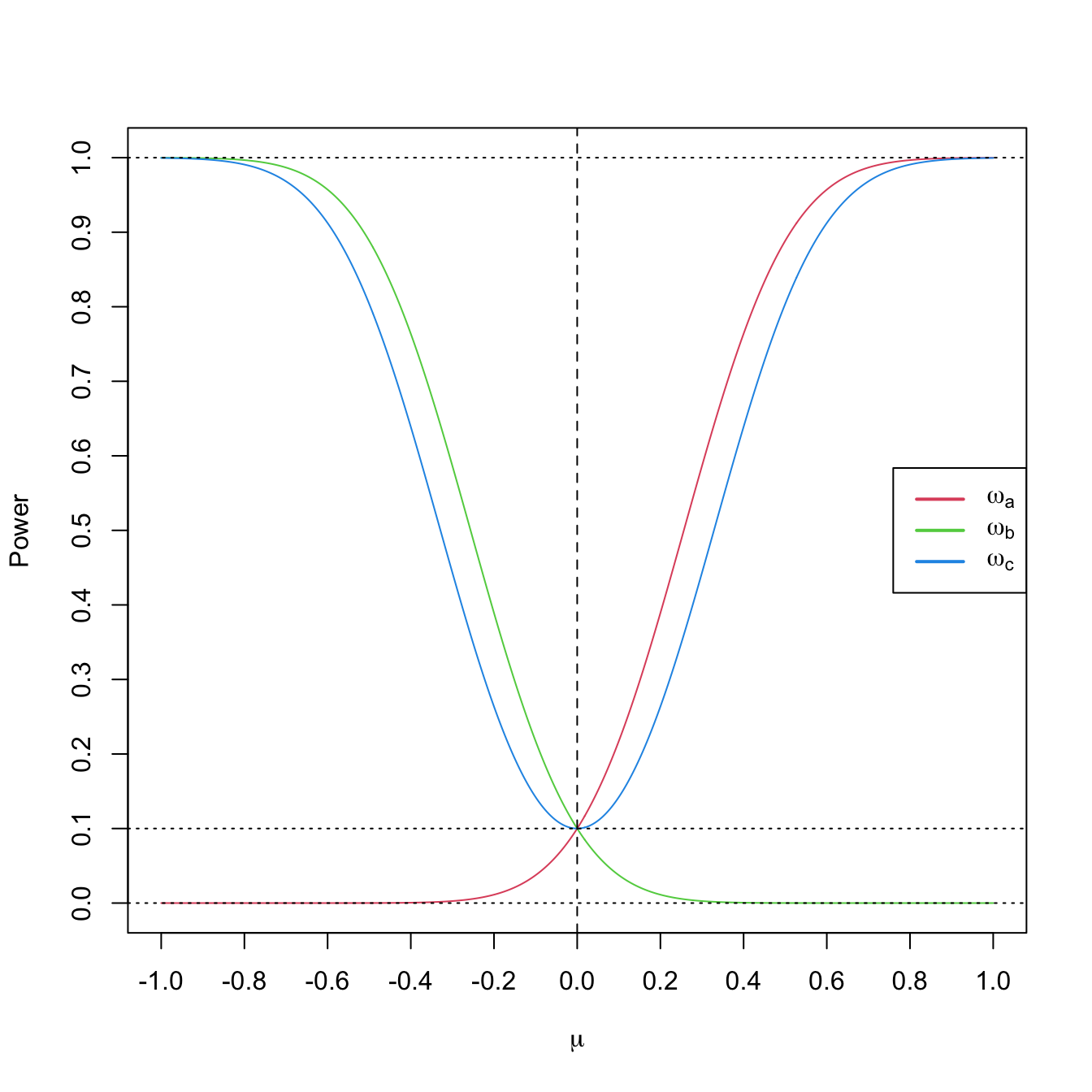
Figure 6.2: Power functions \(\mu\mapsto\omega_a(\mu),\) \(\mu\mapsto\omega_b(\mu),\) and \(\mu\mapsto\omega_c(\mu)\) from Example 6.18 with \(\mu_0=0\) (dashed vertical line), \(\alpha=0.10\) (dotted horizontal line), \(n=25,\) and \(\sigma=1.\) Observe how a one-sided test has power below \(\alpha\) against alternatives in the opposite direction and how the two-sided test almost merges the powers of the two one-sided tests.

The usual criterion for selecting among several types of tests for the same hypothesis consists in fixing the Type I error probability, \(\alpha,\) and then selecting among the tests with the same Type I error the one that presents the highest power for all \(\theta_1\in\Theta_1.\) This is the so-called Uniformly Most Powerful (UMP) test. However, the UMP test does not always exists.

The Neyman–Pearson’s Lemma guarantees the existence of the UMP test for the testing problem in which the null and the alternative hypotheses are simple, and provides us the form of the critical region for such a test. This region is based on a ratio of the likelihoods of the two parameter values appearing in \(H_0\) and \(H_1.\)

Theorem 6.1 (Neyman–Pearson’s Lemma) Let \(X\sim F(\cdot;\theta).\) Assume it is desired to test

\[\begin{align} H_0:\theta=\theta_0\quad \text{vs.}\quad H_1:\theta=\theta_1 \tag{6.5} \end{align}\]

using the information of a srs \((X_1,\ldots,X_n)\) of \(X.\) For the significance level \(\alpha,\) the test that maximizes the power in \(\theta_1\) has a critical region of the form

\[\begin{align*} C=\left\{(x_1,\ldots,x_n)^\top\in\mathbb{R}^n:\frac{\mathcal{L}(\theta_0;x_1,\ldots,x_n)}{\mathcal{L}(\theta_1;x_1,\ldots,x_n)}<k\right\}. \end{align*}\]

Recall that the Neyman–Pearson’s Lemma specifies only the form of the critical region, but not the specific value of \(k.\) However, \(k\) could be computed from the significance level \(\alpha\) and the distribution of \((X_1,\ldots,X_n)\) under \(H_0.\)

Example 6.19 Assume that \(X\) represents a single observation of the rv with pdf

\[\begin{align*} f(x;\theta)=\begin{cases} \theta x^{\theta-1}, & 0<x<1,\\ 0, & \text{otherwise}. \end{cases} \end{align*}\]

Find the UMP test at a significance level \(\alpha=0.05\) for testing

\[\begin{align*} H_0: \theta=1\quad \text{vs.} \quad H_1:\theta=2. \end{align*}\]

Let us employ Theorem 6.1. In this case we have a srs of size one. Then, the likelihood is

\[\begin{align*} \mathcal{L}(\theta;x)=\theta x^{\theta-1}. \end{align*}\]

For computing the critical region of the UMP test, we obtain

\[\begin{align*} \frac{\mathcal{L}(\theta_0;x)}{\mathcal{L}(\theta_1;x)}=\frac{\mathcal{L}(1;x)}{\mathcal{L}(2;x)}=\frac{1}{2x} \end{align*}\]

and therefore

\[\begin{align*} C=\left\{x\in\mathbb{R}:\frac{1}{2x}<k\right\}=\left\{x>\frac{1}{2k}\right\}=\{x>k'\}. \end{align*}\]

The value of \(k'\) can be determined from the significance level \(\alpha,\)

\[\begin{align*} \alpha&=\mathbb{P}(\text{Reject $H_0$} \mid \text{$H_0$ true})=\mathbb{P}(X>k'|\theta=1)\\ &=\int_{k'}^1 f(x;1)\,\mathrm{d}x=\int_{k'}^{1}\,\mathrm{d}x=1-k'. \end{align*}\]

Therefore, \(k'=1-\alpha,\) so the critical region of UMP test of size \(\alpha\) is

\[\begin{align*} C=\{x:x>1-\alpha\}. \end{align*}\]

When testing one-sided hypothesis of the type

\[\begin{align} H_0:\theta=\theta_0\quad \text{vs.}\quad H_1:\theta>\theta_0,\tag{6.6} \end{align}\]

the Neyman–Pearson’s Lemma is not applicable.

However, if we fix a value \(\theta_1>\theta_0\) and we compute the critical region of the UMP test for

\[\begin{align*} H_0:\theta=\theta_0\quad \text{vs.}\quad H_1:\theta=\theta_1, \end{align*}\]

quite often the critical region obtained does not depend on the value \(\theta_1.\) Therefore, this very same test is the UMP test for testing (6.6)!

In addition, if we have an UMP test for

\[\begin{align*} H_0:\theta=\theta_0\quad \text{vs.}\quad H_1:\theta>\theta_0, \end{align*}\]

then the same test is also the UMP test for

\[\begin{align*} H_0:\theta=\theta_0'\quad \text{vs.}\quad H_1:\theta>\theta_0, \end{align*}\]

since for any value \(\theta_0'<\theta_0,\) any other test will have larger errors of the two types.

6.7 The likelihood ratio test

Definition 6.7 (Likelihood ratio test) Let

\[\begin{align*} H_0:\boldsymbol{\theta}\in\Theta_0\quad \text{vs.}\quad H_1:\boldsymbol{\theta}\in\Theta_1, \end{align*}\]

be a testing problem where \(\Theta_0\) and \(\Theta_1\) are complementary subsets of the parameter space, i.e., such that \(\Theta_1=\bar{\Theta}_0.\)⁸⁰ For a srs \((X_1,\ldots,X_n)\) from \(F(\cdot;\theta),\) let \(\mathcal{L}(\hat{\boldsymbol{\theta}}_0;X_1,\ldots,X_n)\) be the maximized likelihood attained inside \(\Theta_0,\) that is,

\[\begin{align*} \mathcal{L}(\hat{\boldsymbol{\theta}}_0;X_1,\ldots,X_n)=\sup_{\boldsymbol{\theta}\in\Theta_0}\mathcal{L}(\boldsymbol{\theta};X_1,\ldots,X_n), \end{align*}\]

and, with the same notation, let \(\mathcal{L}(\hat{\boldsymbol{\theta}};X_1,\ldots,X_n)\) be the maximum likelihood attained inside \(\Theta.\) The Likelihood Ratio Test (LRT) is defined as the test with critical region of the form

\[\begin{align*} C=\left\{(x_1,\ldots,x_n)^\top\in\mathbb{R}^n:\frac{\mathcal{L}(\hat{\boldsymbol{\theta}}_0;x_1,\ldots,x_n)}{\mathcal{L}(\hat{\boldsymbol{\theta}};x_1,\ldots,x_n)}\leq k\right\}. \end{align*}\]

The quantity

\[\begin{align*} \lambda_n:=\frac{\mathcal{L}(\hat{\boldsymbol{\theta}}_0;X_1,\ldots,X_n)}{\mathcal{L}(\hat{\boldsymbol{\theta}};X_1,\ldots,X_n)} \end{align*}\]

is referred to as the likelihood ratio statistic.

Remark. Note that the rejection region is at the left because a small \(\lambda_n\) indicates that \(\mathcal{L}(\hat{\boldsymbol{\theta}}_0;X_1,\ldots,X_n)\ll \mathcal{L}(\hat{\boldsymbol{\theta}};X_1,\ldots,X_n),\) i.e., that the null hypothesis \(H_0\) is unlikely given the data.

The likelihood ratio test is a generalization of the Neyman–Pearson’s Lemma. In fact, if \(\Theta=\{\theta_0,\theta_1\},\) \(\Theta_0=\{\theta_0\},\) and \(\Theta_1=\{\theta_1\},\) then the LRT is equivalent to the UMP test for (6.5). In the following theorem, however, \(\Theta_1=\{\theta_1\}\) is not allowed.

Theorem 6.2 (Asymptotic distribution of the likelihood ratio statistic) Under certain regularity conditions⁸¹ about \(F(\cdot;\theta)\) the distribution of \(X,\) and under \(H_0,\) it is verified that

\[\begin{align} -2\log\lambda_n\stackrel{d}{\longrightarrow} \chi_p^2, \tag{6.7} \end{align}\]

if \(p=\dim\Theta-\dim\Theta_0\geq 1\) is the number of specified parameters under \(H_0.\)

Remark. Theorem 6.2 is also known as Wilk’s Theorem and result (6.7) is often referred to as a Wilk’s phenomenon (the null distribution of the log-likelihood ratio does not depend on \(\theta\) asymptotically).

The LRT based on \(-2\log\lambda_n\) rejects for large values of the test statistic, as these correspond to small values of \(\lambda_n\) (see the remark after Definition 6.7). Therefore, the asymptotic \(p\)-value for the LRT using the test statistic \(-2\log\lambda_n\) is the upper-tail probability of the \(\chi^2_p\) distribution: \(\mathbb{P}[\chi^2_p>-2\log\lambda_n].\) Note that this is the \(p\)-value for a two-sided test, yet still an upper tail is involved!⁸²

Example 6.20 A labor union registers the number of complaints that are filled per week by the workers of two different shifts in the production line of a factory. The union gathers \(n_1=87\) and \(n_2=61\) independent observations about the number of complaints for both shifts \(X_1\) and \(X_2.\) The means \(\bar{X}_1=20\) and \(\bar{X}_2=22\) result. Assume that the number of complaints per week of the \(k\)-th shift has \(\mathrm{Pois}(\theta_k)\) distribution, \(k=1,2.\) The labor union wants to test if the average number of complaints per week of both shifts is significantly different or not at a significance level \(\alpha=0.01.\)

The hypothesis to test is

\[\begin{align*} H_0:\theta_1=\theta_2\quad \text{vs.} \quad H_1:\theta_1\neq \theta_2. \end{align*}\]

Recall that the parametric space is

\[\begin{align*} \Theta=\{(\theta_1,\theta_2)^\top\in\mathbb{R}^2: \theta_1\geq 0,\theta_2\geq 0\}, \end{align*}\]

and that the space \(\Theta_0\) that determines the null hypothesis is

\[\begin{align*} \Theta_0=\{(\theta_1,\theta_2)\in\mathbb{R}^2: \theta_1=\theta_2\}, \end{align*}\]

so the number of specified parameters is \(p=2-1=1.\)

The pmf of the Poisson of mean \(\theta_k\) is

\[\begin{align*} p(x;\theta_k)=\frac{\theta_k^x e^{-\theta_k}}{x!},\quad x=0,1,2,\ldots \end{align*}\]

Two samples of sizes \(n_1=87\) and \(n_2=61\) were observed, one for each shift, and we denote them by

\[\begin{align*} \boldsymbol{X}_1=(X_{11},\ldots,X_{1n_1})^\top,\quad \boldsymbol{X}_2=(X_{11},\ldots,X_{2n_2})^\top. \end{align*}\]

The joint likelihood is

\[\begin{align*} \mathcal{L}(\theta_1,\theta_2;\boldsymbol{X}_1,\boldsymbol{X}_2)=\frac{\theta_1^{\sum_{i=1}^{n_1}X_{1i}}\theta_2^{\sum_{j=1}^{n_2}X_{2j}}e^{-(n_1\theta_1+n_2\theta_2)}}{c}, \end{align*}\]

where \(c=X_{11}!\cdots X_{1n_1}!X_{11}!\cdots X_{2n_2}!\) does not depend on the parameters.

We compute the maximum likelihood in \(\Theta_0.\) This is attained at the MLE restricted to \(\Theta_0.\) But, under \(H_0:\theta_1=\theta_2=:\theta,\) the likelihood is

\[\begin{align*} \mathcal{L}(\theta;\boldsymbol{X}_1,\boldsymbol{X}_2)=\frac{\theta^{\sum_{i=1}^{n_1}X_{1i}+\sum_{j=1}^{n_2}X_{2j}}e^{-(n_1+n_2)\theta}}{c} \end{align*}\]

Computing the maximum of this likelihood, we obtain the MLE restricted to \(\Theta_0.\) Taking the log-likelihood

\[\begin{align*} \ell(\theta;\boldsymbol{X}_1,\boldsymbol{X}_2)=\left(\sum_{i=1}^{n_1}X_{1i}+\sum_{j=1}^{n_2}X_{2j}\right)\log\theta -(n_1+n_2)\theta-\log c \end{align*}\]

and differentiating and equating to zero, we have

\[\begin{align*} \hat{\theta}_0=\frac{\sum_{i=1}^{n_1}X_{1i}+\sum_{j=1}^{n_2}X_{2j}}{n_1+n_2}=\frac{n_1 \bar{X}_{1}+n_2 \bar{X}_{2}}{n_1+n_2}. \end{align*}\]

The unrestricted MLE’s of \(\theta_1\) and \(\theta_2\) are obtained from the unrestricted log-likelihood, which is

\[\begin{align*} \ell(\theta_1,\theta_2;\boldsymbol{X}_1,\boldsymbol{X}_2)=\left(\sum_{i=1}^{n_1} X_{1i}\right) \log\theta_1+\left(\sum_{j=1}^{n_2} X_{2j}\right) \log\theta_2-(n_1\theta_1+n_2\theta_2)-\log c. \end{align*}\]

Differentiating and equating to zero, we have

\[\begin{align*} \hat{\theta}_1=\bar{X}_1,\quad \hat{\theta}_2=\bar{X}_2. \end{align*}\]

Then, the maximum likelihoods in \(\Theta_0\) and \(\Theta\) are, respectively,

\[\begin{align*} \mathcal{L}(\hat{\theta}_0;\boldsymbol{X}_1,\boldsymbol{X}_2) &=\frac{\hat{\theta}_0^{n_1\bar{X}_1+n_2\bar{X}_2}e^{-(n_1+n_2)\hat{\theta}_0}}{c},\\ \mathcal{L}(\hat{\theta}_1,\hat{\theta}_2;\boldsymbol{X}_1,\boldsymbol{X}_2)&=\frac{\hat{\theta}_1^{n_1\bar{X}_1}\hat{\theta}_2^{n_2\bar{X}_2}e^{-(n_1\hat{\theta}_1+n_2\hat{\theta}_2)}}{c}. \end{align*}\]

Therefore, the likelihood ratio statistic is

\[\begin{align*} \lambda_n=\frac{\mathcal{L}(\hat{\theta}_0;\boldsymbol{X}_1,\boldsymbol{X}_2)}{\mathcal{L}(\hat{\theta}_1,\hat{\theta}_2 ;\boldsymbol{X}_1,\boldsymbol{X}_2)}=\frac{\hat{\theta}_0^{n_1\bar{X}_1+n_2\bar{X}_2}}{\hat{\theta}_1^{n_1\bar{X}_1}\hat{\theta}_2^{n_2\bar{X}_2}}e^{-(n_1+n_2)\hat{\theta}_0+(n_1\hat{\theta}_1+n_2\hat{\theta}_2)} \end{align*}\]

and the log-likelihood ratio statistic is

\[\begin{align*} \log\lambda_n=&\;(n_1\bar{X}_1+n_2\bar{X}_2)\log(\hat{\theta}_0)-(n_1\bar{X}_1)\log(\hat{\theta}_1)-(n_2\bar{X}_2)\log(\hat{\theta}_2)\\ &-(n_1+n_2)\hat{\theta}_0+n_1\hat{\theta}_1+n_2\hat{\theta}_2. \end{align*}\]

We use R to compute \(-2\log\lambda_n\):

# Data
xbar_1 <- 20
xbar_2 <- 22
n_1 <- 87
n_2 <- 61

# MLE's under H0 and H1
theta_hat_0 <- (n_1 * xbar_1 + n_2 * xbar_2) / (n_1 + n_2)
theta_hat_1 <- xbar_1
theta_hat_2 <- xbar_2

# Log-likelihood ratio statistic
log_lamba_n <- (n_1 * xbar_1 + n_2 * xbar_2) * log(theta_hat_0) -
  (n_1 * xbar_1) * log(theta_hat_1) - (n_2 * xbar_2) * log(theta_hat_2) -
  (n_1 + n_2) * theta_hat_0 + (n_1 * theta_hat_1 + n_2 * theta_hat_2)
-2 * log_lamba_n
## [1] 6.851838

Then, \(-2\log\lambda_n\approx6.85>\chi_{1;0.01}^2\approx6.635.\) Therefore, \(H_0:\theta_1=\theta_2\) is rejected, that is, the data indicate that the average number of complaints in both shifts differ significantly. In addition, since the \(p\)-value of the test is

# p-value of the test
pchisq(-2 * log_lamba_n, df = 1, lower.tail = FALSE)
## [1] 0.008855011

we will also reject for any significance level \(\alpha>0.0089.\)

Example 6.21 Derive the LRT for \(H_0:\theta=\theta_0\) vs. \(H_1:\theta\neq\theta_0\) for a srs \((X_1,\ldots,X_n)\sim\mathrm{Exp}(1/\theta).\) For \(\theta_0=1.5,\) compute the \(p\)-value of the test for the sample realizations (1.69, 1.15, 2.66, 0.06, 0.11) and (1.05, 0.72, 1.66, 0.04, 0.07, 0.4, 0.39) using R. What are the rejection decisions for \(\alpha=0.05\)?

First, from Exercise 4.11 we know that

\[\begin{align*} \ell(\theta;X_1,\ldots,X_n)=-n\log\theta-\frac{n\bar{X}}{\theta} \end{align*}\]

and that the unrestricted MLE of \(\theta\) is \(\hat{\theta}_\mathrm{MLE}=\bar{X}.\)

We now obtain \(-2\log\lambda_n.\) Since \(\Theta_0=\{\theta_0\}\) and \(\Theta_1=\{\theta\in\mathbb{R}_+: \theta\neq\theta_0\},\) then \(\hat{\theta}_0=\theta_0,\) i.e., there is no estimation involved under \(H_0.\) Therefore: \[\begin{align*} -2\log\lambda_n=-2\log\frac{\mathcal{L}(\theta_0;X_1,\ldots,X_n)}{\mathcal{L}(\hat{\theta};X_1,\ldots,X_n)}=-2(\ell(\theta_0;X_1,\ldots,X_n)-\ell(\hat{\theta};X_1,\ldots,X_n)), \end{align*}\]

where \(\hat{\theta}\) is obtained by maximizing the log-likelihood under \(\Theta,\) giving \(\hat{\theta}=\hat{\theta}_\mathrm{MLE}=\bar{X}.\)

We are now ready to compute \(-2\log\lambda_n\) with the help of R:

# Log-likelihood
log_lik <- function(x, theta) {
  n <- length(x)
  -n * log(theta) - n * mean(x) / theta
}

# Estimator function
theta_hat <- function(x) {
  mean(x)
}

# theta_0
theta_0 <- 1.5

# Statistic and p-value for first sample
x <- c(1.69, 1.15, 2.66, 0.06, 0.11)
(log_lambda_n <- -2 * (log_lik(x = x, theta = theta_0) -
                         log_lik(x = x, theta = theta_hat(x = x))))
## [1] 0.357139
pchisq(q = log_lambda_n, df = 1, lower.tail = FALSE)
## [1] 0.5500995

# Statistic and p-value for second sample
x <- c(1.05, 0.72, 1.66, 0.04, 0.07, 0.4, 0.39)
(log_lambda_n <- -2 * (log_lik(x = x, theta = theta_0) -
                         log_lik(x = x, theta = theta_hat(x = x))))
## [1] 4.174641
pchisq(q = log_lambda_n, df = 1, lower.tail = FALSE)
## [1] 0.04103325

In conclusion, we do not reject \(H_0\) in the first sample and we reject in the second sample for \(\alpha=0.05.\)

Exercises

Exercise 6.1 A chemical process has produced, until the previous week, on average, \(800\) tons of a chemical product per day. The daily productions this week were \(785,\) \(805,\) \(790,\) \(793,\) and \(802\) tons. Is this data indicating that the average production has gone below the \(800\) tons? Answer by carrying out the adequate hypothesis test at significance level \(\alpha=0.05\) assuming that the daily productions follow a normal distribution.

Exercise 6.2 A study was conducted by the Florida Fish and Wildlife Conservation Commission for estimating the quantity of DDT found in the brain tissues of brown pelicans. Samples of \(n_1=10\) young pelicans and \(n_2=13\) baby pelicans gave the results indicated in the table below (measurements in parts per million). Normality is assumed in both populations, as well as equal variances.

Young pelicans	Baby pelicans
\(n_1=10\)	\(n_2=13\)
\(\bar{X}_1=0.041\)	\(\bar{X}_2=0.026\)
\(S_1'=0.021\)	\(S_2'=0.006\)

1. Test the hypothesis of no difference in the average DDT quantities found in young and baby pelicans against the alternative that the young pelicans show a higher average, with \(\alpha=0.05.\)
2. Is there evidence that the average quantity of DDT for young pelicans is larger than the one for baby pelicans in more than \(0.01\) parts per million?

Exercise 6.3 The hourly salaries of a particular industry have a normal distribution with mean \(\mu=33000\) (in euros/year, before taxes). If in that industry there is a company of \(n=40\) employees that pays an average of \(30500\) euros/year and has a quasistandard deviation on the salaries of \(S'=6250,\) can this company be accused of systematically paying inferior salaries? Employ the significance level \(\alpha=0.01.\)

Exercise 6.4 After an increment of \(8.5\%\) due to inflation in 2023, the average pension in the “régimen general” in Spain in 2023 is \(18305.84\) euros/year. The maximum pension is \(42823.34\) euros/year. The minimum wage is \(15120\) euros/year. All figures are before taxes.

A study conducted by a union of young professionals obtained the following data about the gross yearly salary of professionals in the age range 20–29. The data is divided into two groups of professionals according to their career status:

• Group A: 20708, 21630, 15670, 17764, 19308, 19053, 19196, 18341, 19002, 18459, 19577, 19603, 16950, 17254, 17439, 18507, 18421, 16148, 21317, 18076, 21774, 18920, 16742, 15120, 15120, 17610, 19122, 19956, 19876, 17588, 17309, 19843, 16826, 17088, 17740, 20648, 16064, 19990, 15924, 17079.
• Group B: 35261, 37821, 32167, 41367, 42732, 49535, 38236, 49175, 46720, 34275, 39510, 37475, 42905, 46869, 43089, 30767, 44708, 39449, 40953, 42604, 41246, 39125, 48394, 37166, 44107, 41153, 42399, 45076, 38372, 37798, 36956, 44789, 34909, 44991, 35470.

Answer the following questions using significance level \(\alpha=0.05\):

1. Are professionals in Group A better paid than the average pension? And worse paid than the maximum pension?
2. Repeat the previous question for Group B.
3. Pool the data together and answer the questions in a.

Exercise 6.5 A researcher is convinced that his measuring device has a variability equal to a standard deviation of \(2\) measurement units. Seventeen measurements gave as a result \(S'^2=6.1.\) Assuming normality, does the data agree or disagree with his belief? Determine the \(p\)-value of the test and the test decision at the significance level \(\alpha=0.05.\)

Exercise 6.6 The delivery times of two fast-food chains within a neighborhood are compared. The delivery times (in minutes) of \(n_1=13\) orders of chain A and \(n_2=18\) orders of chain B are given below. Assuming normality, is there evidence that the delivery times of chain A are more variable than those of chain B? Employ \(\alpha=0.05.\)

• Chain A: 16.3, 16.6, 14.8, 14, 16.4, 10.9, 16.4, 14.4, 14.4, 12.9, 14.7, 19.1, 15.8.
• Chain B: 16.9, 17.2, 14.7, 13.6, 16.9, 9.3, 17, 14.1, 14.1, 12.1, 14.6, 20.7, 16.2, 16.6, 12.6, 17.6, 12.2, 14.

Exercise 6.7 A psychological study was carried out in order to compare the response times (in seconds) of men and women with respect to a certain stimulus. Two independent srs’s of \(42\) men and \(45\) women were employed in the experiment. The results are shown in the table. Is the data showing enough evidence for suggesting a difference between the average response for men and women? Employ \(\alpha=0.05.\)

Men	Women
\(n_1=42\)	\(n_2=45\)
\(\bar{X}_1=3.6\)	\(\bar{X}_2=3.8\)
\(S_1'^2=0.18\)	\(S_2'^2=0.14\)

Exercise 6.8 Two surveys were conducted by the Centro de Investigaciones Sociológicas (CIS), in May 2023 and July 2023. In them, the percentage of Spaniards that self-identify as middle class (“Clase media-media”) are \(47.2\%\) and \(48.7\%,\) respectively. The sample sizes on each poll are \(4030\) and \(4164.\) Using a significance level of \(1\%,\) can we guarantee that this increment is significant?

Exercise 6.9 In the July 2023 survey of the CIS it was asked to which political party the respondent voted in the Spanish General Elections of 2019. There were \(3585\) respondents. The results for the five national parties are shown in the table below, along with the percentage of votes actually received at the general elections.

Political party	Declared 2023	Received 2019
PSOE	\(31.20\%\)	\(28.25\%\)
PP	\(20.30\%\)	\(20.99\%\)
VOX	\(6.60\%\)	\(15.21\%\)
PODEMOS-IU	\(13.30\%\)	\(12.97\%\)
Cs	\(6.10\%\)	\(6.86\%\)

We want to investigate the social bias in the answers of the respondents to the interviewers.

1. For all political parties, test the equality of same proportion of votes as declared in 2023 and as received in 2019. What are the obtained \(p\)-values? What are your conclusions?
2. Which voting preferences, if any, are significantly underreported? Which ones are overreported? Use a significance level of \(1\%.\)

Exercise 6.10 Two manufacturers, A and B, compete for the supply of batteries for a known company of electric cars, E. Company E has been told by manufacturer B that its batteries are more reliable than those from manufacturer A, the current supplier of batteries for E. To test this statement, company E is presented with historical data from the reliability of \(n_B=1736\) batteries produced by B for a smaller brand, with only \(7\) batteries requiring service before five years. Company E checks this reliability against the historical data of its production line using A’s batteries, where \(n_A=21239\) and \(191\) batteries have required service before five years. At significance level \(\alpha=0.01,\) should the company E change its supplier to have a higher reliability?

Exercise 6.11 The closing prices of two common stocks were recorded during a period of \(16\) days:

• Stock 1: 38.83, 40.67, 41.68, 37.42, 40.86, 40.96, 39.62, 39.65, 39.63, 39.23, 39.74, 39.09, 39.37, 40.41, 41.52, 40.19.
• Stock 2: 42.76, 43.93, 44.08, 41.71, 44.27, 43.73, 40.12, 41.6, 43.22, 44.83, 41.69, 44.16, 45.42, 44.7, 42.04, 44.21.

Is this data showing enough evidence indicating a difference in variability for the closing prices of the two stocks? Determine the \(p\)-value of the test. What would be concluded with \(\alpha=0.02\)? Assume normality (although stock prices are typically not normally distributed).

Exercise 6.12 A local brewery intends to buy a new bottling machine and considers two models, A and B, manufactured by different companies. The decisive factor for buying one model or the other is the variability in the filling of the bottles; the machine with the lower variance is the preferred one. To infer the machines’ filling variances, \(10\) bottles are filled in each one, obtaining the results of the table below. Perform the three types of tests (right one-sided, left one-sided, and two-sided) at the significance level \(\alpha=0.05\) for the null hypothesis of equality of variances of the two machines (assume normality). What are your conclusions?

A	B
\(n_A=10\)	\(n_B=10\)
\(\bar{X}_A=0.9\)	\(\bar{X}_B=0.93\)
\(S_A'^2=0.04\)	\(S_B'^2=0.03\)

Exercise 6.13 The Weibull distribution with parameters \(\lambda>0\) and \(k>0\) has pdf

\[\begin{align*} f(x;\lambda,k)=\frac{k}{\lambda}\left(\frac{x}{\lambda}\right)^{k-1}e^{-(x/\lambda)^k}, \quad x>0. \end{align*}\]

Estimate \(\lambda\) by maximum likelihood assuming \(k=2\) and estimate the Fisher information of \(\lambda.\) Then, obtain the \(p\)-values of the tests for

1. \(H_0:\lambda=1\) vs. \(H_1:\lambda>1\) and
2. \(H_0:\lambda=1\) vs. \(H_1:\lambda\neq 1\)

for the sample realization 1.66, 0.94, 1.54, 1.27, 1.78, 1.85, 2.34, 1.74, 1.32, 0.6, 0.88, 2.33, 1.49, 0.7, 0.73, 2.32, 1.92, 2.6, 2.51, 2.09, 3.09, 1.1, 1.76, 2.74, 2.1, 0.73, 1.47.

Exercise 6.14 Assume a srs from a negative binomial distribution \(\mathrm{NB}(r,p)\) (Exercise 5.24) is given and that \(r>0\) is known. Derive the critical region of an asymptotic test for \(H_0:p=p_0\) vs. \(H_1:p\neq p_0.\)

Exercise 6.15 The growth coefficient of certain bacteria follows a log-normal distribution \(\mathcal{LN}(\mu,\sigma^2)\) (see Exercise 5.19). The volume of bacteria in a Petri dish typically duplicates every hour, which means that their growth coefficient is \(2.\) Since the expectation of \(\mathcal{LN}(\mu,\sigma^2)\) is \(\exp(\mu+\sigma^2/2),\) this means that \(\mu+\sigma^2/2=\log(2).\)

A researcher suspects that exposing the bacteria to a chemical can slow down their growth. In \(30\) experiments, he exposes the bacteria to the chemical and annotates their growth coefficients: 1.46, 1.23, 2.34, 1.44, 1.79, 1.4, 2.18, 1.4, 1.79, 1.06, 1.38, 1.31, 1.78, 1.39, 1.41, 1.88, 1.51, 2.42, 2.13, 2.02, 2.32, 1.01, 1.28, 0.93, 1.6, 1.69, 3.37, 2.1, 2, 1.81.

Conduct a hypothesis test to check whether the growth coefficient of the bacteria is significantly lower from \(2\) at significance level \(\alpha=0.05\) and report the \(p\)-value. The parameter of interest for the hypothesis test is \(\theta:=\mu+\sigma^2/2.\) Hint: exploit result (4.7) on multiparameter inference for the vector \((\mu,\sigma^2)^\top,\) then use a linear transformation to have an asymptotic result for \(\theta,\) and then construct a test using \(\hat{\boldsymbol{\mathcal{I}}}(\hat{\mu}_\mathrm{MLE},\hat{\sigma}_\mathrm{MLE}^2).\)

Exercise 6.16 Assume a srs \((X_1,\ldots,X_n)\) of a continuous rv \(X\) and an arbitrary test statistic \(T(X_1,\ldots,X_n)\stackrel{H_0}{\sim}F_T.\) Prove that the \(p\)-value of the test is a rv distributed as \(\mathcal{U}(0,1)\) under \(H_0.\) Do it for each of the following testing problems:

1. \(H_0:\theta=\theta_0\) vs. \(H_1:\theta>\theta_0.\)
2. \(H_0:\theta=\theta_0\) vs. \(H_1:\theta<\theta_0.\)
3. \(H_0:\theta=\theta_0\) vs. \(H_1:\theta\neq\theta_0.\)

Exercise 6.17 Replicate Figure 6.2 in R. Once you have a working solution, explore the following parameters for arbitrary fixed values of the others:

1. \(n=5,50,200.\)
2. \(\sigma=0.1,2,10.\)
3. \(\mu_0=-1,5,10.\)

In each case, describe the changes of the power curves and interpret the reason of these changes.

Exercise 6.18 Build the analogous example to Example 6.18 for:

1. \(H_0:\sigma^2=\sigma_0^2\) vs. \(H_1:\sigma^2\neq\sigma_0^2.\)
2. \(H_0:\sigma^2=\sigma_0^2\) vs. \(H_1:\sigma^2>\sigma_0^2.\)
3. \(H_0:\sigma^2=\sigma_0^2\) vs. \(H_1:\sigma^2<\sigma_0^2.\)

Assume normal populations. The chi-square cdf is available as pchisq() in R. The resulting figure for the right one-sided test should be similar to Figure 6.1. Do you observe any strange behavior? Can you explain it?

Exercise 6.19 Approximate by Monte Carlo the power curves displayed in Figure 6.2 for the case where \(\sigma\) is unknown. To do so, approximate the rejection probability in \(\omega(\mu)\) by the relative rejection frequency of the corresponding test using \(M\) random samples, for each \(\mu\) in a sequence. You can use the following pseudocode as a guiding template:

For mu_i in mu
    For j in 1:M
        Draw sample of size n from N(mu_i, sigma^2)
        Test H0: mu = mu0 vs. H1
        Save test decision
    End
    rel_freq_i <- Relative rejection frequency
End
Draw (mu, rel_freq)

Use \(M=1000\) and the same settings of Figure 6.2. You may use the t.test() function in R to carry out one-sample tests for \(H_0:\mu=\mu_0.\)

Exercise 6.20 Assume that \(X_1\sim\mathcal{N}(\mu,\sigma_1^2)\) and \(X_2\sim\mathcal{N}(\mu,\sigma_2^2).\) Denote \(\theta=\sigma_1^2/\sigma_2^2.\) Let \((X_{11},\ldots,X_{1n_1})\) and \((X_{21},\ldots,X_{2n_2})\) be two srs’s of \(X_1\) and \(X_2,\) respectively. Using Monte Carlo, as explained in Exercise 6.19, obtain and draw the power curves for:

1. \(H_0:\theta=1\) vs. \(H_1:\theta>1.\)
2. \(H_0:\theta=1\) vs. \(H_1:\theta<1.\)
3. \(H_0:\theta=1\) vs. \(H_1:\theta\neq1.\)

Consider \(n_1=25\) and \(n_2=50.\) Use \(M=1000\) and the sequence of \(\theta\) given by theta <- seq(0.1, 10, l = 25).

Exercise 6.21 Find the UMP test for \(H_0:\theta=\theta_0\) vs. \(H_1:\theta=\theta_1\) in a \(\mathrm{Exp}(\theta)\) distribution. Then, obtain the \(p\)-value of such a test for:

1. \(\theta_0=1\) and \(\theta_1=0.5\) with the sample realization (0.8, 0.2, 1.8, 1.3, 3.8, 0.4, 1.6, 2, 0.4, 1.4, 0.1, 0.6, 2, 2.3, 0.6, 0.2, 0.7, 1.2, 0.3, 1.8, 0.2).
2. \(\theta_0=2\) and \(\theta_1=1\) with the sample realization (1.6, 14, 0, 8.4, 4.9, 1.7, 0.2, 2.6, 0.9, 0.3, 1.6, 1.7, 2.3, 2.2, 5.6, 2.8, 2.6, 0, 2, 2.7, 4).

Exercise 6.22 The following sample from a \(\mathcal{N}(0,\sigma^2)\) distribution is given: 0, -1.6, 1.4, -0.1, -0.3, 0.5, 0.6, -1.1, 0.1, -1.4, -1.7, 2.8, 2.2, -1, 0.5, 1.1, 1.3, 0.5, 1.2, 0.4, 0.4, -2.2, -0.7, -1.5, -0.7, -1, -0.3, 2.8, 1, -0.9, -0.7, -1.5, 1.2, 0.8.

1. Find the UMP test for \(H_0:\sigma=1\) vs. \(H_1:\sigma=2.\) Report the \(p\)-value of the above test when applied to the sample.
2. Repeat part a for \(H_0:\sigma=1\) vs. \(H_1:\sigma=\sigma_1\) with \(\sigma_1=0.75,1.5.\)
3. Plot the \(p\)-value curve of the test as a function of \(\sigma_1>0\) for \(H_0:\sigma=1\) vs. \(H_1:\sigma=\sigma_1.\)

Exercise 6.23 Validate the asymptotic distribution (6.7) of the likelihood ratio statistic in Theorem 6.2 by Monte Carlo. To do so, first derive and implement the likelihood ratio statistic \(\lambda_n\) for the following testing problems:

1. \(H_0:\theta=0\) vs. \(H_1:\theta\neq0\) with \((X_1,\ldots,X_n)\sim\mathcal{N}(\theta,1).\)
2. \(H_0:\theta=1\) vs. \(H_1:\theta\neq1\) with \((X_1,\ldots,X_n)\sim\mathrm{Exp}(\theta).\)
3. Example 6.20 with \(\theta_1=\theta_2=0.5\) and \(n_1=n_2=n.\)

Then, show a histogram of \(-2\log\lambda_n\) by Monte Carlo and overlay the pdf of \(\chi^2_p.\) Use \(M=1000\) and \(n=10,50,100,500.\) Use the dchisq() function in R to plot the pdf of a chi-square rv.

Exercise 6.24 Let \((X_{11},\ldots,X_{1n_1})\) and \((X_{21},\ldots,X_{2n_2})\) be two srs’s from two independent normal populations \(\mathcal{N}(\mu_1,\sigma_1^2)\) and \(\mathcal{N}(\mu_2,\sigma_2^2),\) respectively. Let us test the equality of populations, that is,

\[\begin{align*} H_0:(\mu_1,\sigma_1^2)=(\mu_2,\sigma_2^2)\quad \text{vs.} \quad H_1:(\mu_1,\sigma_1^2)\neq(\mu_2,\sigma_2^2). \end{align*}\]

1. Derive the LRT for this problem. Use that, under \(H_0,\) \(\hat{\mu}_\mathrm{MLE}=(n_1\bar{X}_1+n_2\bar{X}_2)/(n_1+n_2)\) and \(\hat{\sigma}^2_\mathrm{MLE}=(n_1S^2_1+n_2S^2_2)/(n_1+n_2).\)
2. Implement in R a function to conduct this LRT, returning its \(p\)-value.
3. Check with simulated data that the test works correctly under \(H_0\) (does not reject) and \(H_1\) (rejects).
4. Apply the LRT to the variables iris$Sepal.Width[iris$Species == "versicolor"] and iris$Sepal.Width[iris$Species == "virginica"] from the iris dataset in R.

Exercise 6.25 Let \(\boldsymbol{X}\sim \mathcal{N}_2(\boldsymbol{\mu},\boldsymbol{\Sigma})\) be a bivariate random vector. Assume that the srs \(\boldsymbol{X}_1,\ldots,\boldsymbol{X}_n\) is iid from \(\boldsymbol{X}.\)

1. Derive the LRT for \(H_0:\rho=0\) vs. \(H_1:\rho\neq 0.\) Use that \(\hat{\boldsymbol{\mu}}_\mathrm{MLE}=\bar{\boldsymbol{X}}\) and \(\hat{\boldsymbol{\Sigma}}_\mathrm{MLE}=\frac{1}{n}\sum_{i=1}^n (\boldsymbol{X}_i-\bar{\boldsymbol{X}})(\boldsymbol{X}_i-\bar{\boldsymbol{X}})^\top.\)
2. Implement in R a function to conduct this LRT, returning its \(p\)-value.
3. Check with simulated data that the test works correctly under \(H_0\) (does not reject) and \(H_1\) (rejects). Use mvtnorm::rmvnorm() to simulate from a bivariate normal distribution.
4. Apply the LRT to the variables Sepal.Length and Sepal.Width from the iris dataset in R.

References

Lehmann, E. L., and J. P. Romano. 2005. Testing Statistical Hypotheses. Third. Springer Texts in Statistics. New York: Springer. https://doi.org/10.1007/0-387-27605-X.

---

74. For the so-called two-sided tests, to be introduced in Section 6.2, \(\Theta_0=\{\theta_0\},\) \(\Theta_1=\bar{\Theta}_0,\) and \(\Theta_2=\emptyset.\) However, for the so-called one-sided tests, \(\Theta_0=\{\theta_0\},\) \(\Theta_1=(\theta_0,+\infty),\) and \(\Theta_2=(-\infty, \theta_0)\) (or \(\Theta_1=(-\infty,\theta_0)\) and \(\Theta_2=(\theta_0,+\infty)\)).↩︎

75. Therefore, under \(H_0\) the distribution of \(X\) is completely known.↩︎

76. What will be \(\alpha\) and \(\beta\) for the rejection region \(C=\{Y\geq 10\}\)?↩︎

77. In some textbooks it is sometimes written \(H_0:\mu\leq\mu_0\) vs. \(H_1:\mu > \mu_0.\) However, this notation introduces inconsistencies when determining the distribution of the test statistic under \(H_0,\) as then several values for \(\mu\) are possible. For that reason it is avoided.↩︎

78. A good exercise is to check that this statement is true using and that the outcomes of t.test(x, y, paired = TRUE) and t.test(x - y, mu = 0) are equivalent.↩︎

79. In this case, the distributions of \(T\) and \(-T\) are equal!↩︎

80. Note that this setup rules out one-sided tests where \(\bar{\Theta}_0\neq\Theta_1.\)↩︎

81. See the list at Theorem 12.4.2 in Lehmann and Romano (2005).↩︎

82. An explanation for this different behavior of two-sided tests is that here we are working on with test statistics based on differences of log-likelihoods, rather than in terms of differences (or ratios) of parameters and estimators, as done with normal-, CLT-, and MLE-based two-sided tests.↩︎