1 Preliminaries

This first chapter contains a probability review and the required machinery for subsequent chapters. Particularly relevant are random vectors and their transformations, and the moment generating function.

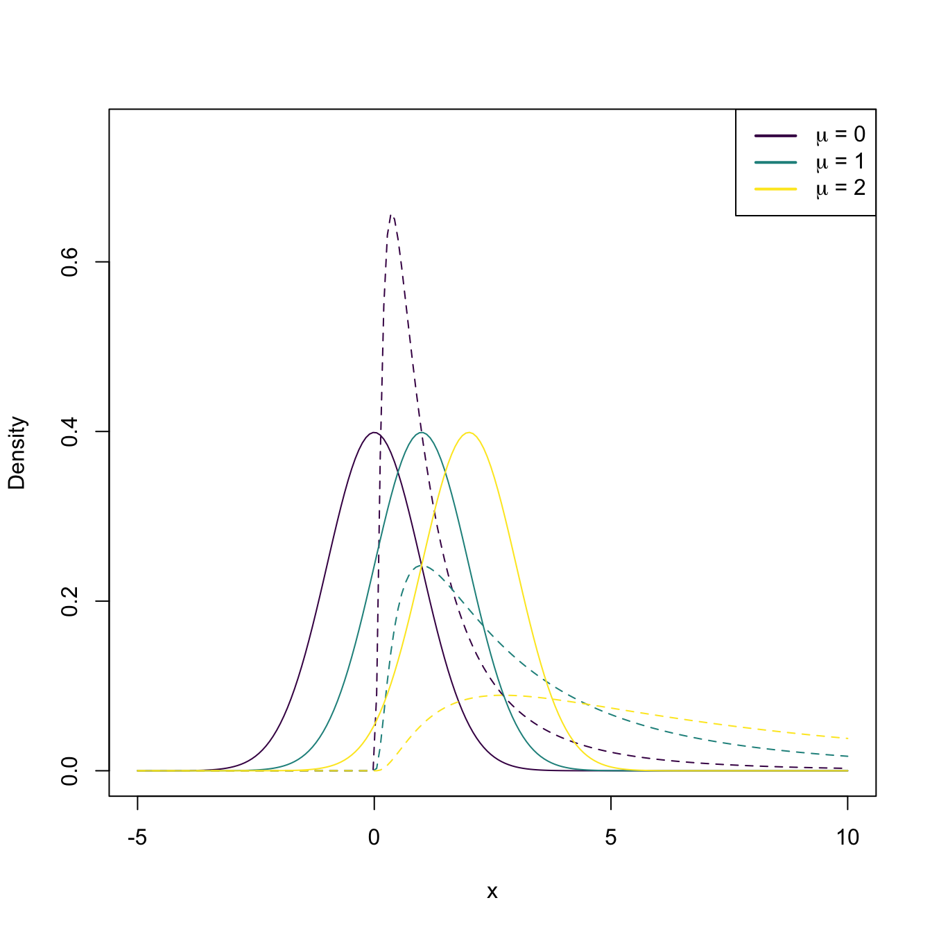
Figure 1.1: The pdf of \(X\sim\mathcal{N}(\mu,1)\) (solid lines) and the pdf of \(Y=X^2\) (dashed lines), for a range of values of \(\mu\).

1.1 Probability review

The following probability review starts with the very conceptualization of “randomness” through the random experiment, introduces the set theory needed for probability functions, and introduces the three increasingly general definitions of probability.

1.1.1 Random experiment

Definition 1.1 (Random experiment) A random experiment \(\xi\) is an experiment with the following properties:

• its outcome is impossible to predict;
• if the experiment is repeated under the same conditions, the outcome may be different;
• the set of possible outcomes is known in advance.

The following concepts are associated with a random experiment:

• The set of possible outcomes of \(\xi\) is termed as the sample space and is denoted as \(\Omega.\)
• The individual outcomes of \(\xi\) are called sample outcomes, realizations, or elements, and are denoted by \(\omega\in\Omega.\)
• An event \(A\) is a subset of \(\Omega.\) Once the experiment has been performed, it is said that \(A\) “happened” if the individual outcome of \(\xi,\) \(\omega,\) belongs to \(A.\)

Example 1.1 The following are random experiments:

1. \(\xi=\) “Tossing a coin”. The sample space is \(\Omega=\{\mathrm{H},\mathrm{T}\}\) (Heads, Tails). Some events are: \(\emptyset,\) \(\{\mathrm{H}\},\) \(\{\mathrm{T}\},\) \(\Omega.\)
2. \(\xi=\) “Measuring the number of car accidents within an hour in Spain”. The sample space is \(\Omega=\mathbb{N}\cup\{0\}.\)
3. \(\xi=\) “Measuring the weight (in kgs) of a pedestrian between \(20\) and \(40\) years old”. The sample space is \(\Omega=[m,\infty),\) where \(m\) is a certain minimum weight.

1.1.2 Borelians and measurable spaces

A probability function will be defined as a mapping of subsets (events) of the sample space \(\Omega\) to elements in \([0,1].\) Therefore, it is necessary to count on a “good” structure for these subsets in order to generate “good” properties for the probability function. A \(\sigma\)-algebra gives such a structure.

Definition 1.2 (\(\sigma\)-algebra) A \(\sigma\)-algebra \(\mathcal{A}\) over a set \(\Omega\) is a collection of subsets of \(\Omega\) with the following properties:

1. \(\emptyset\in \mathcal{A};\)
2. If \(A\in\mathcal{A},\) then \(\overline{A}\in \mathcal{A},\) where \(\overline{A}\) is the complement of \(A;\)
3. If \(\{A_i\}_{i=1}^\infty\subset\mathcal{A},\) then \(\cup_{n=1}^{\infty} A_i\in \mathcal{A}.\)

A \(\sigma\)-algebra \(\mathcal{A}\) over \(\Omega\) defines a collection of sets that is closed under intersections and unions, i.e., it is impossible to take sets on \(\mathcal{A},\) operate on them through unions and intersections thereof, and end up with a set that does not belong to \(\mathcal{A}.\)

The following are two commonly employed \(\sigma\)-algebras.

Definition 1.3 (Discrete \(\sigma\)-algebra) The discrete \(\sigma\)-algebra of the set \(\Omega\) is the power set \(\mathcal{P}(\Omega):=\{A:A\subset \Omega\},\) that is, the collection of all subsets of \(\Omega.\)

Definition 1.4 (Borel \(\sigma\)-algebra) Let \(\Omega=\mathbb{R}\) and consider the collection of intervals

\[\begin{align*} \mathcal{I}:=\{(-\infty,a]: a\in \mathbb{R}\}. \end{align*}\]

The Borel \(\sigma\)-algebra, denoted by \(\mathcal{B},\) is defined as the smallest \(\sigma\)-algebra that contains \(\mathcal{I}.\)

Remark. The smallest \(\sigma\)-algebra coincides with the intersection of all \(\sigma\)-algebras containing \(\mathcal{I}.\)

Remark. The Borel \(\sigma\)-algebra \(\mathcal{B}\) contains all the complements, countable intersections, and countable unions of elements of \(\mathcal{I}.\) Particularly, \(\mathcal{B}\) contains all kinds of intervals, isolated points of \(\mathbb{R},\) and unions thereof. For example:

• \((a,\infty)\in\mathcal{B},\) since \((a,\infty)=\overline{(-\infty,a]},\) and \((-\infty,a]\in\mathcal{B}.\)
• \((a,b]\in\mathcal{B},\) \(\forall a<b,\) since \((a,b]=(-\infty,b]\cap (a,\infty),\) where \((-\infty,b]\in\mathcal{B}\) and \((a,\infty)\in\mathcal{B}.\)
• \(\{a\}\in\mathcal{B},\) \(\forall a\in\mathbb{R},\) since \(\{a\}=\bigcap_{n=1}^{\infty}\big(a-\tfrac{1}{n},a\big],\) which belongs to \(\mathcal{B}.\)

However, \(\mathcal{B}\) is not \(\mathcal{P}(\mathbb{R})\) (indeed, \(\mathcal{B}\varsubsetneq\mathcal{P}(\mathbb{R})\)).

Intuitively, the Borel \(\sigma\)-algebra represents the vast collection of sensible subsets of \(\mathbb{R},\) understanding sensible subsets as those constructed with set operations on intervals, which are very well-behaved sets. The emphasis on sensible is important: \(\mathcal{P}(\mathbb{R}),\) on which \(\mathcal{B}\) is contained, is a space populated also by monster sets, such as the Vitali set. We want to be far away from them!

When the sample space \(\Omega\) is continuous and is not \(\mathbb{R},\) but a subset of \(\mathbb{R},\) we need to define a \(\sigma\)-algebra over the subsets of \(\Omega.\)

Definition 1.5 (Restricted Borel \(\sigma\)-algebra) Let \(A\subset \mathbb{R}.\) The Borel \(\sigma\)-algebra restricted to \(A\) is defined as

\[\begin{align*} \mathcal{B}_{A}:=\{B\cap A: B\in\mathcal{B}\}. \end{align*}\]

The \(\sigma\)-algebra \(\mathcal{A}\) over \(\Omega\) gives the required set structure to be able to measure the “size” of the sets with a probability function.

Definition 1.6 (Measurable space) The pair \((\Omega,\mathcal{A}),\) where \(\Omega\) is a sample space and \(\mathcal{A}\) is a \(\sigma\)-algebra over \(\Omega,\) is referred to as a measurable space.

Example 1.2 The measurable space for the experiment \(\xi=\) “Tossing a coin” described in Example 1.1 is

\[\begin{align*} \Omega=\{\mathrm{H}, \mathrm{T}\}, \quad \mathcal{A}=\{\emptyset,\{\mathrm{H}\},\{\mathrm{T}\},\Omega\}. \end{align*}\]

The sample space for experiment \(\xi=\) “Measuring the number of car accidents within an hour in Spain” is \(\Omega=\mathbb{N}_0,\) where \(\mathbb{N}_0=\mathbb{N}\cup \{0\}.\) Taking the \(\sigma\)-algebra \(\mathcal{P}(\Omega),\) then \((\Omega, \mathcal{P}(\Omega))\) is a measurable space.

For experiment \(\xi=\) “Measuring the weight (in kgs) of a pedestrian between \(20\) and \(40\) years old”, in which the sample space is \(\Omega=[m,\infty)\subset\mathbb{R},\) an adequate \(\sigma\)-algebra is the Borel \(\sigma\)-algebra restricted to \(\Omega,\) \(\mathcal{B}_{[m,\infty)}.\)

1.1.3 Probability definitions

A probability function maps an element of the \(\sigma\)-algebra to a real number in the interval \([0,1].\) Thus, probability functions are defined on measurable spaces and will assign a “measure” (called probability) to each set. We will see this formally in Definition 1.9, after seeing some examples and more intuitive definitions next.

Example 1.3 The following tables show the relative frequencies of the outcomes of the random experiments of Example 1.1 when those experiments are repeated \(n\) times.

1. Tossing a coin \(n\) times. Table 1.1 and Figure 1.2 show that the relative frequencies of both “heads” and “tails” converge to \(0.5.\)

   Table 1.1: Relative frequencies of “heads” and “tails” for \(n\) random experiments.

   \(n\)	Heads	Tails
   10	0.300	0.700
   20	0.500	0.500
   30	0.433	0.567
   100	0.380	0.620
   1000	0.495	0.505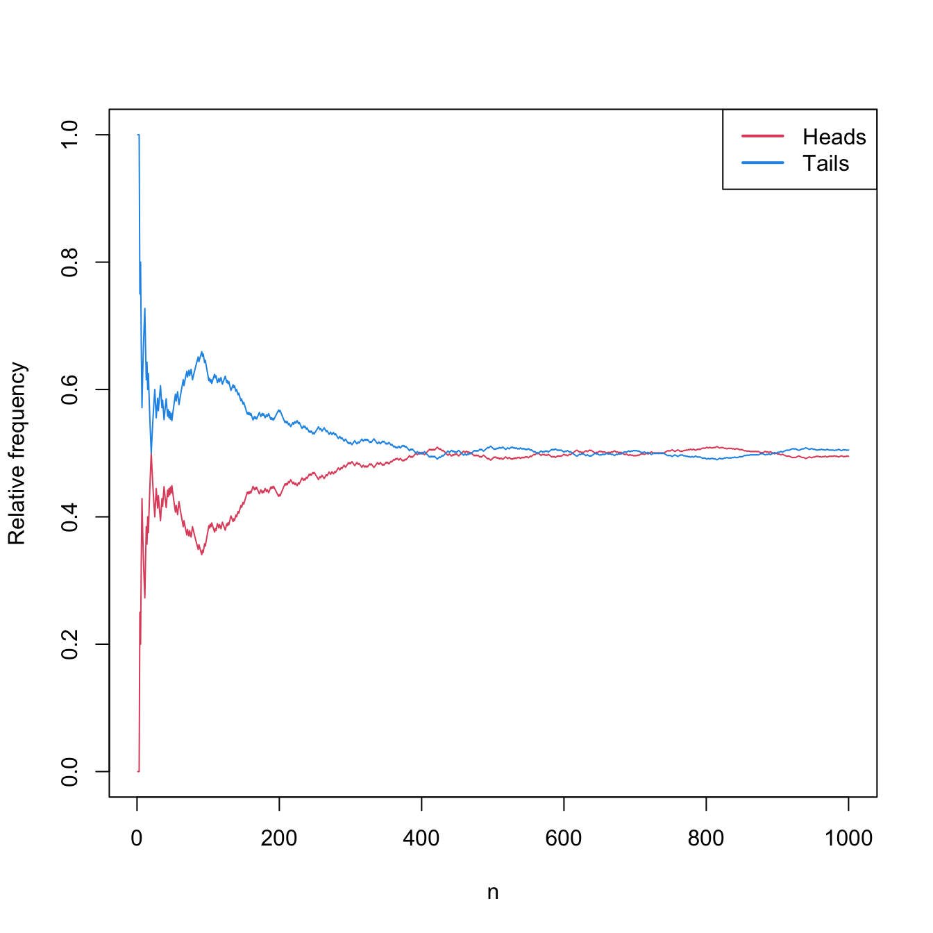

   

   Figure 1.2: Convergence of the relative frequencies of “heads” and “tails” to \(0.5\) as the number of random experiments \(n\) grows.

2. Measuring the number of car accidents for \(n\) independent hours in Spain (simulated data). Table 1.2 and Figure 1.3 show the convergence of the relative frequencies of the experiment.

   Table 1.2: Relative frequencies of car accidents in Spain for \(n\) hours.

   \(n\)	\(0\)	\(1\)	\(2\)	\(3\)	\(4\)	\(5\)	\(\geq 6\)
   10	0.000	0.000	0.300	0.300	0.100	0.100	0.200
   20	0.000	0.000	0.200	0.200	0.100	0.100	0.400
   30	0.000	0.033	0.267	0.133	0.100	0.100	0.367
   100	0.030	0.040	0.260	0.140	0.160	0.110	0.260
   1000	0.021	0.078	0.145	0.192	0.200	0.150	0.214
   10000	0.018	0.074	0.149	0.193	0.194	0.159	0.213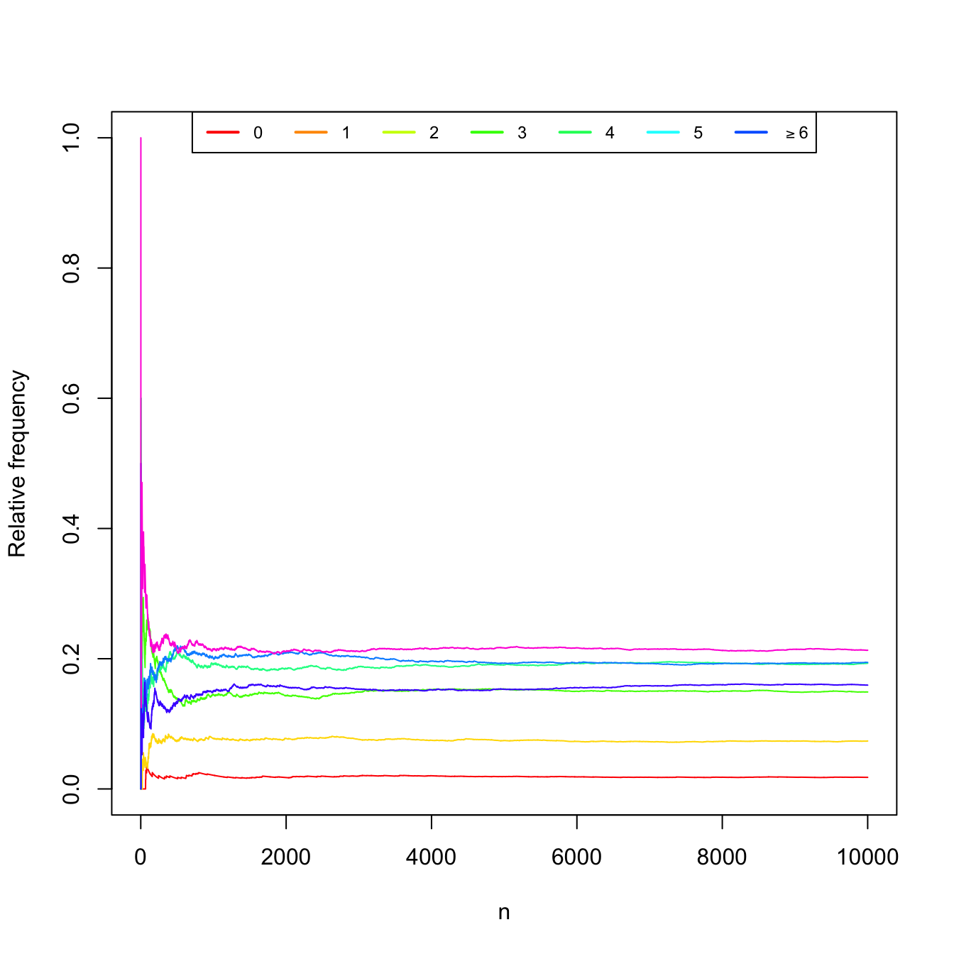

   

   Figure 1.3: Convergence of the relative frequencies of car accidents as the number of measured hours \(n\) grows.

3. Measuring the weight (in kgs) of \(n\) pedestrians between \(20\) and \(40\) years old. Again, Table 1.3 and Figure 1.4 show the convergence of the relative frequencies of the weight intervals.

   Table 1.3: Relative frequencies of weight intervals for \(n\) measured pedestrians.

   \(n\)	\([0, 35)\)	\([35, 45)\)	\([45, 55)\)	\([55, 65)\)	\([65, \infty)\)
   10	0.000	0.000	0.700	0.300	0.000
   20	0.000	0.100	0.700	0.200	0.000
   30	0.000	0.067	0.767	0.167	0.000
   100	0.000	0.220	0.670	0.110	0.000
   1000	0.003	0.200	0.690	0.107	0.000
   5000	0.003	0.207	0.676	0.113	0.001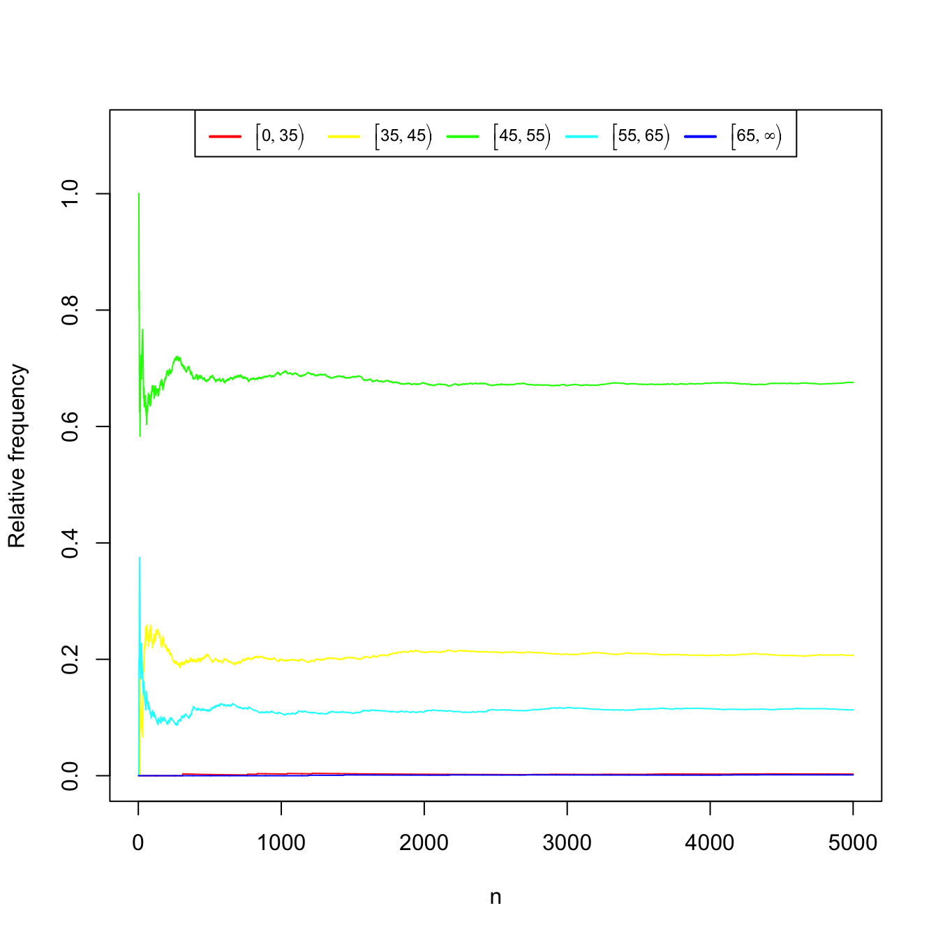

   

   Figure 1.4: Convergence of the relative frequencies of the weight intervals as the number of measured pedestrians \(n\) grows.

As hinted from the previous examples, the frequentist definition of the probability of an event is the limit of the relative frequency of that event when the number of repetitions of the experiment tends to infinity.

Definition 1.7 (Frequentist definition of probability) The frequentist definition of the probability of an event \(A\) is

\[\begin{align*} \mathbb{P}(A):=\lim_{n\to\infty} \frac{n_A}{n}, \end{align*}\]

where \(n\) stands for the number of repetitions of the experiment and \(n_A\) is the number of repetitions in which \(A\) happens.

The Laplace definition of probability can be employed for experiments that have a finite number of possible outcomes, and whose results are equally likely.

Definition 1.8 (Laplace definition of probability) The Laplace definition of probability of an event \(A\) is the proportion of favorable outcomes to \(A,\) that is,

\[\begin{align*} \mathbb{P}(A):=\frac{\# A}{\# \Omega}, \end{align*}\]

where \(\#\Omega\) is the number of possible outcomes of the experiment and \(\# A\) is the number of outcomes in \(A.\)

Finally, the Kolmogorov axiomatic definition of probability does not establish the probability as a unique function, as the previous probability definitions do, but presents three axioms that must be satisfied by any so-called “probability function”.¹

Definition 1.9 (Kolmogorov definition of probability) Let \((\Omega,\mathcal{A})\) be a measurable space. A probability function is a mapping \(\mathbb{P}:\mathcal{A}\rightarrow \mathbb{R}\) that satisfies the following axioms:

1. (Non-negativity) \(\forall A\in\mathcal{A},\) \(\mathbb{P}(A)\geq 0;\)
2. (Unitarity) \(\mathbb{P}(\Omega)=1;\)
3. (\(\sigma\)-additivity) For any sequence \(A_1,A_2,\ldots\) of disjoint events (\(A_i\cap A_j=\emptyset,\) \(i\neq j\)) of \(\mathcal{A},\) it holds

\[\begin{align*} \mathbb{P}\left(\bigcup_{n=1}^{\infty} A_n\right)=\sum_{n=1}^{\infty} \mathbb{P}(A_n). \end{align*}\]

Observe that the \(\sigma\)-additivity property is well-defined: since \(\mathcal{A}\) is a \(\sigma\)-algebra, then the countable union belongs to \(\mathcal{A}\) also, and therefore the probability function takes as argument a proper element from \(\mathcal{A}.\) For this reason the closedness property of \(\mathcal{A}\) under unions, intersections, and complements is especially important.

Definition 1.10 (Probability space) A probability space is a trio \((\Omega,\mathcal{A}, \mathbb{P}),\) where \(\mathbb{P}\) is a probability function defined on the measurable space \((\Omega,\mathcal{A}).\)

Example 1.4 Consider the first experiment described in Example 1.1 with the measurable space \((\Omega,\mathcal{A}),\) where

\[\begin{align*} \Omega=\{\mathrm{H},\mathrm{T}\}, \quad \mathcal{A}=\{\emptyset,\{\mathrm{H}\},\{\mathrm{T}\},\Omega\}. \end{align*}\]

A probability function is \(\mathbb{P}_1:\mathcal{A}\rightarrow[0,1],\) defined as

\[\begin{align*} \mathbb{P}_1(\emptyset):=0, \ \mathbb{P}_1(\{\mathrm{H}\}):=\mathbb{P}_1(\{\mathrm{T}\}):=1/2, \ \mathbb{P}_1(\Omega):=1. \end{align*}\]

It is straightforward to check that \(\mathbb{P}_1\) satisfies the three definitions of probability. Consider now \(\mathbb{P}_2:\mathcal{A}\rightarrow[0,1]\) defined as

\[\begin{align*} \mathbb{P}_2(\emptyset):=0, \ \mathbb{P}_2(\{\mathrm{H}\}):=p<1/2, \ \mathbb{P}_2(\{\mathrm{T}\}):=1-p, \ \mathbb{P}_2(\Omega):=1. \end{align*}\]

If the coin is fair, then \(\mathbb{P}_2\) does not satisfy the frequentist definition nor the Laplace definition, since the outcomes are not equally likely. However, it does verify the Kolmogorov axiomatic definition. Several probability functions, as well as several probability spaces, are mathematically possible! But, of course, some are more sensible than others according to the random experiment they are modeling.

Example 1.5 We can define a probability function for the second experiment of Example 1.1, with the measurable space \((\Omega,\mathcal{P}(\Omega)),\) in the following way:

• For the individual outcomes, the probability is defined as

\[\begin{align*} \begin{array}{lllll} &\mathbb{P}(\{0\}):=0.018, &\mathbb{P}(\{1\}):=0.074, &\mathbb{P}(\{2\}):=0.149, \\ &\mathbb{P}(\{3\}):=0.193, &\mathbb{P}(\{4\}):=0.194, &\mathbb{P}(\{5\}):=0.159, \\ &\mathbb{P}(\{6\}):=0.106, &\mathbb{P}(\{7\}):=0.057, &\mathbb{P}(\{8\}):=0.028, \\ &\mathbb{P}(\{9\}):=0.022, &\mathbb{P}(\emptyset):=0, &\mathbb{P}(\{i\}):=0,\ \forall i>9. \end{array} \end{align*}\]

• For subsets of \(\Omega\) with more than one element, its probability is defined as the sum of probabilities of the individual outcomes belonging to each subset. This is, if \(A=\{a_1,\ldots,a_n\},\) with \(a_i\in \Omega,\) then the probability of \(A\) is

\[\begin{align*} \mathbb{P}(A):=\sum_{i=1}^n \mathbb{P}(\{a_i\}). \end{align*}\]

This probability function indeed satisfies the Kolmogorov axiomatic definition.

Example 1.6 Consider a modification of the first experiment described in Example 1.1, where now \(\xi=\) “Toss a coin two times”. Then,

\[\begin{align*} \Omega=\{\mathrm{HH},\mathrm{HT},\mathrm{TH},\mathrm{TT}\}. \end{align*}\]

We define

\[\begin{align*} \mathcal{A}_1=\{\emptyset,\{\mathrm{HH}\},\ldots,\{\mathrm{HH},\mathrm{HT}\},\ldots,\{\mathrm{HH},\mathrm{HT},\mathrm{TH}\},\ldots,\Omega\}=\mathcal{P}(\Omega). \end{align*}\]

Recall that the cardinality of \(\mathcal{P}(\Omega)\) is \(\#\mathcal{P}(\Omega)=2^{\#\Omega}.\) This can be easily checked for this example by adding how many events comprised by \(0\leq k\leq4\) outcomes are possible: \(\binom{4}{0}+\binom{4}{1}+\binom{4}{2}+\binom{4}{3}+\binom{4}{4}=(1+1)^4\) (Newton’s binomial). For the measurable space \((\Omega,\mathcal{A}_1),\) a probability function \(\mathbb{P}:\mathcal{A}_1\rightarrow[0,1]\) can be defined as

\[\begin{align*} \mathbb{P}(\{\omega\}):=1/4,\quad \forall \omega\in\Omega. \end{align*}\]

Then, \(\mathbb{P}(A)=\sum_{\omega\in A}\mathbb{P}(\{\omega\}),\) \(\forall A\in\mathcal{A}_1.\) This is a valid probability that satisfies the three Kolmogorov’s axioms (and also the frequentist and Laplace definitions) and therefore \((\Omega,\mathcal{A}_1,\mathbb{P})\) is a probability space.

Another possible \(\sigma\)-algebra for \(\xi\) is \(\mathcal{A}_2=\{\emptyset,\{\mathrm{HH}\},\{\mathrm{HT,TH,TT}\},\Omega\},\) for which \(\mathbb{P}\) is well-defined. Then, another perfectly valid probability space is \((\Omega,\mathcal{A}_2,\mathbb{P}).\) This probability space would not make too much sense for modeling \(\xi,\) since it assumes that the outcome \(\mathrm{HT}\) is impossible, as \(\mathbb{P}(\{\mathrm{HT}\})\) is not defined.

Proposition 1.1 (Basic probability results) Let \((\Omega,\mathcal{A},\mathbb{P})\) be a probability space and \(A,B\in\mathcal{A}.\)

• Probability of the union: \(\mathbb{P}(A\cup B)=\mathbb{P}(A)+\mathbb{P}(B)-\mathbb{P}(A\cap B).\)
• De Morgan’s rules: \(\mathbb{P}(\overline{A\cup B})=\mathbb{P}(\overline{A}\cap \overline{B}),\) \(\mathbb{P}(\overline{A\cap B})=\mathbb{P}(\overline{A}\cup \overline{B}).\)

1.1.4 Conditional probability

Conditioning one event on another allows establishing the dependence between them via the conditional probability function.

Definition 1.11 (Conditional probability) Let \((\Omega,\mathcal{A},\mathbb{P})\) be a probability space and \(A,B\in\mathcal{A}\) with \(\mathbb{P}(B)>0.\) The conditional probability of \(A\) given \(B\) is defined as

\[\begin{align} \mathbb{P}(A \mid B):=\frac{\mathbb{P}(A\cap B)}{\mathbb{P}(B)}.\tag{1.1} \end{align}\]

Definition 1.12 (Independent events) Let \((\Omega,\mathcal{A},\mathbb{P})\) be a probability space and \(A,B\in\mathcal{A}.\) Two events are said to be independent if \(\mathbb{P}(A\cap B)=\mathbb{P}(A)\mathbb{P}(B).\)

Equivalently, \(A,B\in\mathcal{A}\) such that \(\mathbb{P}(A),\mathbb{P}(B)>0\) are independent if \(\mathbb{P}(A \mid B)=\mathbb{P}(A)\) or \(\mathbb{P}(B \mid A)=\mathbb{P}(B)\) (i.e., knowing one event does not affect the probability of the other). Computing probabilities of intersections, if the events are independent, is trivial. The following results are useful for working with conditional probabilities.

Proposition 1.2 (Basic conditional probability results) Let \((\Omega,\mathcal{A},\mathbb{P})\) be a probability space.

• Law of total probability: If \(A_1,\ldots,A_k\) is a partition of \(\Omega\) (i.e., \(\Omega=\cup_{i=1}^kA_i\) and \(A_i\cap A_j=\emptyset\) for \(i\neq j\)) that belongs to \(\mathcal{A},\) \(\mathbb{P}(A_i)>0\) for \(i=1,\ldots,k,\) and \(B\in\mathcal{A},\) then \[\begin{align*} \mathbb{P}(B)=\sum_{i=1}^k\mathbb{P}(B \mid A_i)\mathbb{P}(A_i). \end{align*}\]
• Bayes’ theorem:² If \(A_1,\ldots,A_k\) is a partition of \(\Omega\) that belongs to \(\mathcal{A},\) \(\mathbb{P}(A_i)>0\) for \(i=1,\ldots,k,\) and \(B\in\mathcal{A}\) is such that \(\mathbb{P}(B)>0,\) then \[\begin{align*} \mathbb{P}(A_i \mid B)=\frac{\mathbb{P}(B \mid A_i)\mathbb{P}(A_i)}{\sum_{j=1}^k\mathbb{P}(B \mid A_j)\mathbb{P}(A_j)}. \end{align*}\]

Proving the previous results is not difficult. Also, learning how to do it is a good way of always remembering them.

1.2 Random variables

The random variable concept allows transforming the sample space \(\Omega\) of a random experiment into a set with good mathematical properties, such as the real numbers \(\mathbb{R},\) effectively forgetting spaces like \(\Omega=\{\mathrm{H},\mathrm{T}\}.\)

Definition 1.13 (Random variable) Let \((\Omega,\mathcal{A})\) be a measurable space. Let \(\mathcal{B}\) be the Borel \(\sigma\)-algebra over \(\mathbb{R}.\) A random variable (rv) is a mapping \(X:\Omega\rightarrow \mathbb{R}\) that is measurable, that is, that verifies

\[\begin{align*} \forall B\in\mathcal{B}, \quad X^{-1}(B)\in\mathcal{A}, \end{align*}\]

with \(X^{-1}(B)=\{\omega\in\Omega: X(\omega)\in B\}.\)

The adjective measurable for the mapping \(X:\Omega\rightarrow \mathbb{R}\) simply means that any Borelian \(B\) has been generated through \(X\) with a set (\(X^{-1}(B)\)) that belongs to \(\mathcal{A}\) and therefore measure can be assigned to it.

A random variable transforms a measurable space \((\Omega,\mathcal{A})\) into another measurable space with a more convenient mathematical framework, \((\mathbb{R},\mathcal{B}),\) whose \(\sigma\)-algebra is the one generated by the class of intervals. The measurability condition of the random variable allows one to transfer the probability of any subset \(A\in\mathcal{A}\) to the probability of a subset \(B\in\mathcal{B},\) where \(B\) is precisely the image of \(A\) through the random variable \(X.\) The concept of random variable reveals itself as a key translator: it allows transferring the randomness “produced” by the concept of a random experiment with sample space \(\Omega\) to the mathematically-friendly \((\mathbb{R},\mathcal{B}).\) After this transfer is done, we do not require dealing with \((\Omega,\mathcal{A})\) anymore and we can focus on \((\mathbb{R},\mathcal{B})\) (yet \((\Omega,\mathcal{A})\) is always underneath).³

Remark. The space \((\Omega,\mathcal{A})\) is dependent on \(\xi.\) However, \((\mathbb{R},\mathcal{B})\) is always the same space, irrespective of \(\xi\)!

Example 1.7 For the experiments given in Example 1.1, the next are random variables:

1. A possible random variable for the measurable space \[\begin{align*} \Omega=\{\mathrm{H},\mathrm{T}\}, \quad \mathcal{A}=\{\emptyset,\{\mathrm{H}\},\{\mathrm{T}\},\Omega\}, \end{align*}\] is \[\begin{align*} X(\omega):=\begin{cases} 1, & \mathrm{if}\ \omega=\mathrm{H},\\ 0, & \mathrm{if}\ \omega=\mathrm{T}. \end{cases} \end{align*}\] We can call this random variable “Number of heads when tossing a coin”. Indeed, this is a random variable, since for any subset \(B\in\mathcal{B},\) it holds:
   • If \(0,1\in B,\) then \(X^{-1}(B)=\Omega\in \mathcal{A}.\)
   • If \(0\in B\) but \(1\notin B,\) then \(X^{-1}(B)=\{\mathrm{T}\}\in \mathcal{A}.\)
   • If \(1\in B\) but \(0\notin B,\) then \(X^{-1}(B)=\{\mathrm{H}\}\in \mathcal{A}.\)
   • If \(0,1\notin B,\) then \(X^{-1}(B)=\emptyset\in \mathcal{A}.\)
2. For the measurable space \((\Omega,\mathcal{P}(\Omega)),\) where \(\Omega=\mathbb{N}_0,\) since the sample space is already contained in \(\mathbb{R},\) an adequate random variable is \(X_1(\omega):=\omega.\) Indeed, \(X_1\) is a random variable, because for \(B\in\mathcal{B},\) the set \[\begin{align*} X_1^{-1}(B)=\{\omega\in \mathbb{N}_0: X_1(\omega)=\omega\in B\} \end{align*}\] is the set of natural numbers (including zero) that belong to \(B.\) But any countable set of natural numbers belongs to \(\mathcal{P}(\Omega),\) as this \(\sigma\)-algebra contains all the subsets of \(\mathbb{N}_0.\) Therefore, \(X_1=\) “Number of car accidents within a day in Spain” is a random variable. Another possible random variable is the one that indicates whether there is at least one car accident, and is given by \[\begin{align*} X_2(\omega):=\begin{cases} 1, & \mathrm{if}\ \omega\in \mathbb{N}, \\ 0, & \mathrm{if} \ \omega=0. \end{cases} \end{align*}\] Indeed, \(X_2\) is a random variable, since for \(B\in\mathcal{B}\):
   • If \(0,1\in B,\) then \(X_2^{-1}(B)=\Omega\in \mathcal{P}(\Omega).\)
   • If \(1\in B\) but \(0\notin B,\) then \(X_2^{-1}(B)=\mathbb{N}\in \mathcal{P}(\Omega).\)
   • If \(0\in B\) but \(1\notin B,\) then \(X_2^{-1}(B)=\{0\}\in \mathcal{P}(\Omega).\)
   • If \(0,1\notin B,\) then \(X_2^{-1}(B)=\emptyset\in \mathcal{P}(\Omega).\)
3. As in the previous case, for the measurable space \((\Omega,\mathcal{B}_{\Omega}),\) where \(\Omega=[m,\infty),\) a random variable is \(X_1(\omega):=\omega,\) since for \(B\in \mathcal{B},\) we have \[\begin{align*} X_1^{-1}(B)=\{\omega\in[m,\infty): X_1(\omega)=\omega\in B\}=[m,\infty)\cap B\in \mathcal{B}_{\Omega}. \end{align*}\] \(X_1\) is therefore a random variable that corresponds to the “Weight of a pedestrian between 20 and 40 years old”. Another possible random variable is \[\begin{align*} X_2(\omega):=\begin{cases} 1, & \mathrm{if}\ \omega \geq 65,\\ 0, & \mathrm{if}\ \omega<65, \end{cases} \end{align*}\] which corresponds to the concept “Weight of at least 65 kilograms”.

Example 1.8 Let \(\xi=\) “Draw a point at random from \(\Omega=\{(x,y)^\top\in\mathbb{R}^2:x^2+y^2\leq 1\}\)”. Then, \(\omega=(x,y)^\top\in\Omega\) and we can define the random variable \(X:=\) “Distance to the center of \(\Omega\)” as \(X(\omega)=\sqrt{x^2+y^2}.\) It can be seen (but it is technical) that indeed \(X\) is a proper random variable for the measurable space \((\Omega,\mathcal{B}^2_\Omega),\) where \(\mathcal{B}^2=\{A_1\times A_2:A_1,A_2\in\mathcal{B}\}.\)

The induced probability of a random variable is the probability function defined over subsets of \(\mathbb{R}\) that preserves the probabilities of the original events of \(\Omega.\) This gives the final touch for completely translating the probability space \((\Omega,\mathcal{A},\mathbb{P})\) to the probability space \((\mathbb{R},\mathcal{B},\mathbb{P}_X),\) which is much more manageable.

Definition 1.14 (Induced probability of a rv) Let \(\mathcal{B}\) be the Borel \(\sigma\)-algebra over \(\mathbb{R}.\) The induced probability of the rv \(X\) is the function \(\mathbb{P}_X:\mathcal{B}\rightarrow \mathbb{R}\) defined as

\[\begin{align*} \mathbb{P}_X(B):=\mathbb{P}(X^{-1}(B)), \quad \forall B\in \mathcal{B}. \end{align*}\]

Example 1.9 Consider the probability function \(\mathbb{P}_1\) defined in Example 1.4 and the random variable \(X\) defined in part a in Example 1.7. For \(B\in\mathcal{B},\) the induced probability of \(X\) is described in the following way:

• If \(0,1\in B,\) then \(\mathbb{P}_{1X}(B)=\mathbb{P}_1(X^{-1}(B))=\mathbb{P}_1(\Omega)=1.\)
• If \(0\in B\) but \(1\notin B,\) then \(\mathbb{P}_{1X}(B)=\mathbb{P}_1(X^{-1}(B))=\mathbb{P}_1(\{\mathrm{T}\})=1/2.\)
• If \(1\in B\) but \(0\notin B,\) then \(\mathbb{P}_{1X}(B)=\mathbb{P}_1(X^{-1}(B))=\mathbb{P}_1(\{\mathrm{H}\})=1/2.\)
• If \(0,1\notin B,\) then \(\mathbb{P}_{1X}(B)=\mathbb{P}_1(X^{-1}(B))=\mathbb{P}_1(\emptyset)=0.\)

Therefore, the induced probability by \(X\) is

\[\begin{align*} \mathbb{P}_{1X}(B)=\begin{cases} 0, & \mathrm{if}\ 0,1\notin B,\\ 1/2, & \text{if $0$ or $1$ are in $B$},\\ 1, & \mathrm{if}\ 0,1\in B. \end{cases} \end{align*}\]

Particularly, we have the following probabilities:

• \(\mathbb{P}_{1X}(\{0\})=\mathbb{P}_1(X=0)=1/2.\)
• \(\mathbb{P}_{1X}((-\infty,0])=\mathbb{P}_1(X\leq 0)=1/2.\)
• \(\mathbb{P}_{1X}((0,1])=\mathbb{P}_1(0< X\leq 1)=1/2.\)

Example 1.10 For the probability function \(\mathbb{P}\) defined in Example 1.5 and the random variable \(X_1\) defined in part b in Example 1.7, the induced probability by the random variable \(X_1\) is described in the following way. Let \(B\in\mathcal{B}\) be such that \(\mathbb{N}_0\cap B=\{a_1,a_2,\ldots,a_p\}.\) Then:

\[\begin{align*} \mathbb{P}_{X_1}(B)&=\mathbb{P}(X_1^{-1}(B))=\mathbb{P}_1(\mathbb{N}_0\cap B)\\ &=\mathbb{P}(\{a_1,a_2,\ldots,a_p\})=\sum_{i=1}^p \mathbb{P}(\{a_i\}). \end{align*}\]

In practice, we will not need to compute what is the probability induced \(\mathbb{P}_X\) of a random variable \(X\) that is based on a random experiment \(\xi.\) We will take a shortcut: directly specify \(\mathbb{P}_X\) via a probability model, and forget about the conceptual pillars on which \(X\) and \(\mathbb{P}_X\) are built (the random experiment \(\xi\) and the probability space \((\Omega,\mathcal{A},\mathbb{P})\)). For introducing probability models, we need to distinguish first among the two main types of random variables: discrete and continuous.

1.2.1 Types of random variables

Before diving into the specifics of discrete and continuous variables we introduce the common concept of cumulative distribution function of a random variable \(X.\)

Definition 1.15 (Cumulative distribution function) The cumulative distribution function (cdf) of a random variable \(X\) is the function \(F_X:\mathbb{R}\rightarrow [0,1]\) defined as

\[\begin{align*} F_X(x):=\mathbb{P}_X((-\infty,x]), \quad \forall x\in \mathbb{R}. \end{align*}\]

We will denote \(\mathbb{P}(X\leq x):=\mathbb{P}_X((-\infty,x])\) for simplicity.

Remark. The cdf is properly defined since \((-\infty,x]\in\mathcal{B},\) so \(\mathbb{P}_X((-\infty,x])=\mathbb{P}(X^{-1}((-\infty,x]))\) and since \(X\) is measurable (from the definition of a random variable), then \(X^{-1}((-\infty,x])\in\mathcal{A}\) and \(\mathbb{P}(X^{-1}((-\infty,x]))\) is well-defined.

The following properties are easy to check.

Proposition 1.3 (Properties of the cdf)

1. The cdf is monotonically non-decreasing, that is, \[\begin{align*} x<y \implies F_X(x)\leq F_X(y). \end{align*}\]
2. Let \(a,b\in\mathbb{R}\) such that \(a<b.\) Then, \[\begin{align*} \mathbb{P}(a<X\leq b)=F_X(b)-F_X(a). \end{align*}\]
3. \(\lim_{x\to-\infty} F(x)=0.\)
4. \(\lim_{x\to\infty} F(x)=1.\)
5. \(F_X\) is right-continuous.⁴
6. The set of points where \(F_X\) is discontinuous is finite or countable.

Definition 1.16 (Discrete random variable) A random variable \(X\) is discrete if its range (or image set) \(R_X:=\{x\in \mathbb{R}: x=X(\omega)\ \text{for some} \ \omega\in \Omega\}\) is finite or countable.

Example 1.11 Among the random variables defined in Example 1.7, the ones from parts a and b are discrete, and so is \(X_2\) from part c.

In the case of discrete random variables, we can define a function that gives, in particular, the probabilities of the individual points of its range \(R_X.\)

Definition 1.17 (Probability mass function) The probability mass function (pmf) of a discrete random variable \(X\) is the function \(p_X:\mathbb{R}\rightarrow [0,1]\) defined as

\[\begin{align*} p_X(x):=\mathbb{P}_X(\{x\}), \quad \forall x\in \mathbb{R}. \end{align*}\]

We will denote \(\mathbb{P}(X=x):=\mathbb{P}_X(\{x\})\) for simplicity.

With the terminology “distribution of a discrete random variable \(X\)” we refer to either the probability function induced by \(X,\) \(\mathbb{P}_X,\) the cdf \(F_X,\) or the pmf \(p_X.\) The motivation for this abuse of notation is that any of these functions completely determines the random behavior of \(X.\)

Definition 1.18 (Continuous random variable) A continuous random variable \(X\) (more precisely denoted absolutely continuous⁵) is the one whose cdf \(F_X\) is expressible as

\[\begin{align} F_X(x)=\int_{-\infty}^x f_X(t)\,\mathrm{d}t,\quad\forall x\in\mathbb{R},\tag{1.2} \end{align}\]

where \(f_X:\mathbb{R}\rightarrow[0,\infty).\) The function \(f_X\) is the probability density function (pdf) of \(X.\) Sometimes the pdf is simply referred to as the density function.

Example 1.12 The random variable \(X_1=\) “Weight of a pedestrian between 20 and 40 years old”, defined in part c of Example 1.7, is continuous.

The pdf is called like that because, for any \(x\in\mathbb{R},\) it measures the density of the probability of an infinitesimal interval centered at \(x.\)

Proposition 1.4 (Properties of the pdf)

1. \(F_X'(x)=f_X(x)\) for almost all \(x\in\mathbb{R}.\)⁶
2. \(f_X\) is such that \[\begin{align*} \int_{-\infty}^{\infty} f_X(t)\,\mathrm{d}t=1. \end{align*}\]
3. For \(A\in\mathcal{B},\) \(\mathbb{P}(X\in A)=\int_{A} f_X(t)\,\mathrm{d}t.\)⁷

As in the discrete case, a continuous random variable \(X\) is fully determined by either the induced probability function \(\mathbb{P}_X,\) the cdf \(F_X,\) or the pdf \(f_X.\) Therefore, whenever we refer to the “distribution of a random variable”, we may be referring to any of these functions.

Remark. Observe that, for a discrete random variable \(X,\) the cdf \(F_X\) can be obtained by the pmf \(p_X\) in an analogous way to (1.2):

\[\begin{align*} F_X(x)=\sum_{\{x_i\in\mathbb{R}:p_X(x_i)>0,\,x_i\leq x\}}p_X(x_i). \end{align*}\]

Remark. Recall that the cdf accumulates probability irrespective of the type of the random variable. It does not assign probability to specific values of \(X;\) this is a type-dependent operation:

• If \(X\) is discrete, the assignment of probability is done by the pmf \(p_X.\) The values that \(X\) can take with positive probability are called atoms.
• If \(X\) is continuous, the assignment of infinitesimal probability is done by the pdf \(f_X.\) There are no atoms in a continuous random variable, since \(\mathbb{P}(X=x)=\int_x^xf_X(t)\,\mathrm{d}t=0\) for any \(x\in\mathbb{R}.\)

We will write \(X\sim F\) to denote that the random variable \(X\) has cdf \(F.\) In other words, the symbol “\(\sim\)” (tilde) stands for “distributed as”. Sometimes \(F\) is denoted by a more evocative symbol representing the distribution, as illustrated in the following examples.

Example 1.13 (Uniform (discrete)) The random variable \(X\sim\mathcal{U}(\{1,\ldots,N\})\) is such that its pmf is

\[\begin{align*} p(x;N)=\frac{1}{N},\quad x=1,\ldots,N. \end{align*}\]

Example 1.14 (Poisson model) The random variable \(X\sim\mathrm{Pois}(\lambda),\) \(\lambda>0\) (intensity parameter), is such that its pmf is

\[\begin{align*} p(x;\lambda)=\frac{e^{-\lambda}\lambda^x}{x!},\quad x=0,1,2,\ldots \end{align*}\]

The points \(\{0,1,2,\ldots\}\) are the atoms of \(X.\) This probability model is useful to model counts.

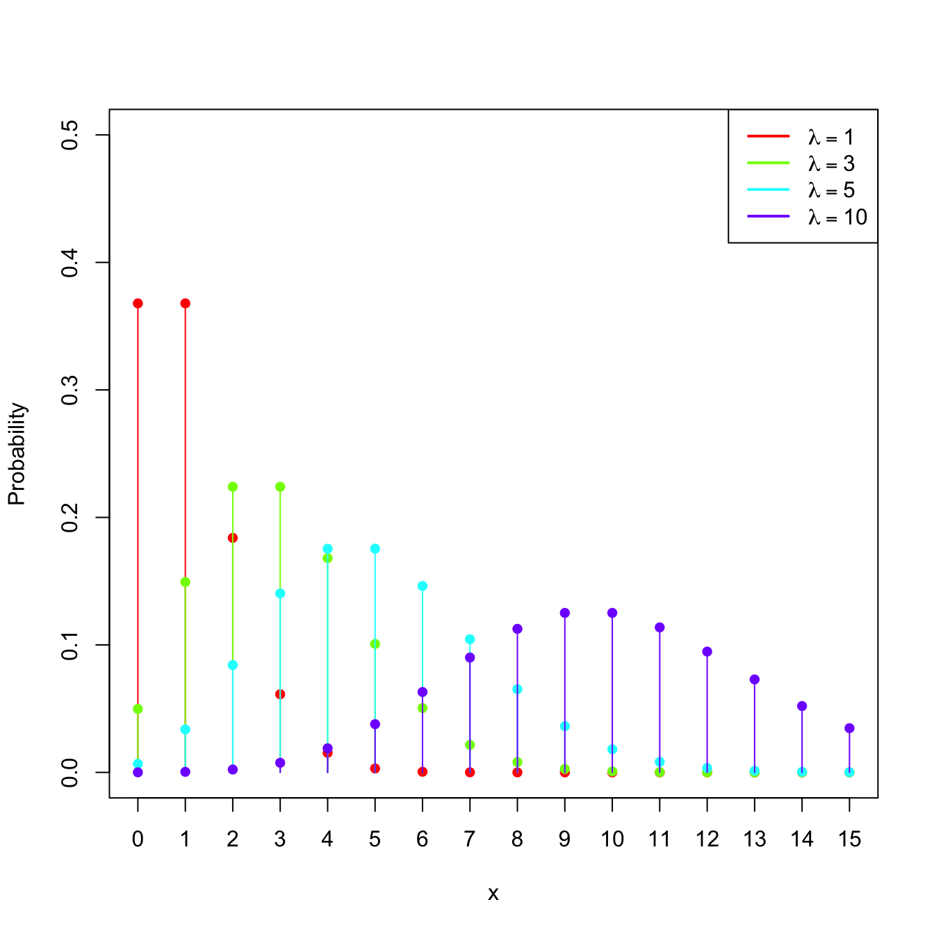
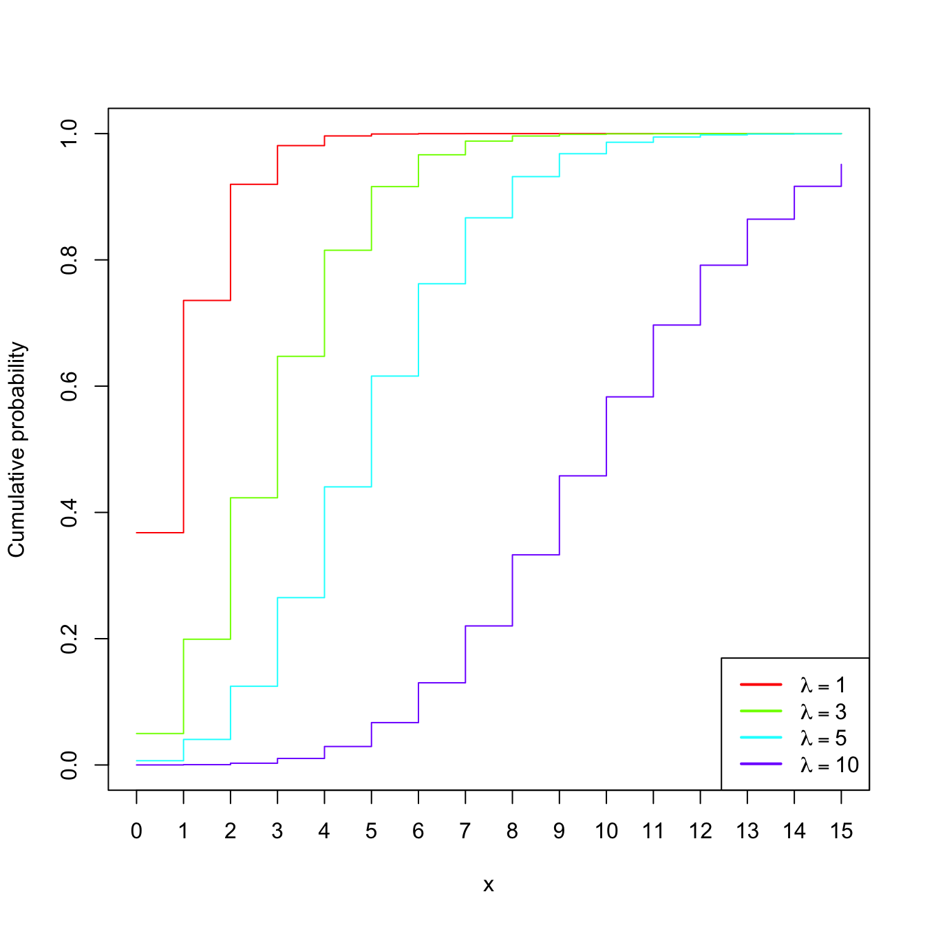
Figure 1.5: \(\mathrm{Pois}(\lambda)\) pmf’s and cdf’s for several intensities \(\lambda.\)

Example 1.15 (Binomial model) The random variable \(X\sim\mathrm{Bin}(n,p),\) with \(n\in\mathbb{N}\) and \(p\in[0,1],\) is such that its pmf is

\[\begin{align*} p(x;n,p)=\binom{n}{x}p^x(1-p)^{n-x},\quad x=0,1,\ldots,n. \end{align*}\]

The points \(\{0,1,\ldots,n\}\) are the atoms of \(X.\) This probability model is designed to sum the successes of a random experiment with probability of success \(p\) that is independently repeated \(n\) times.

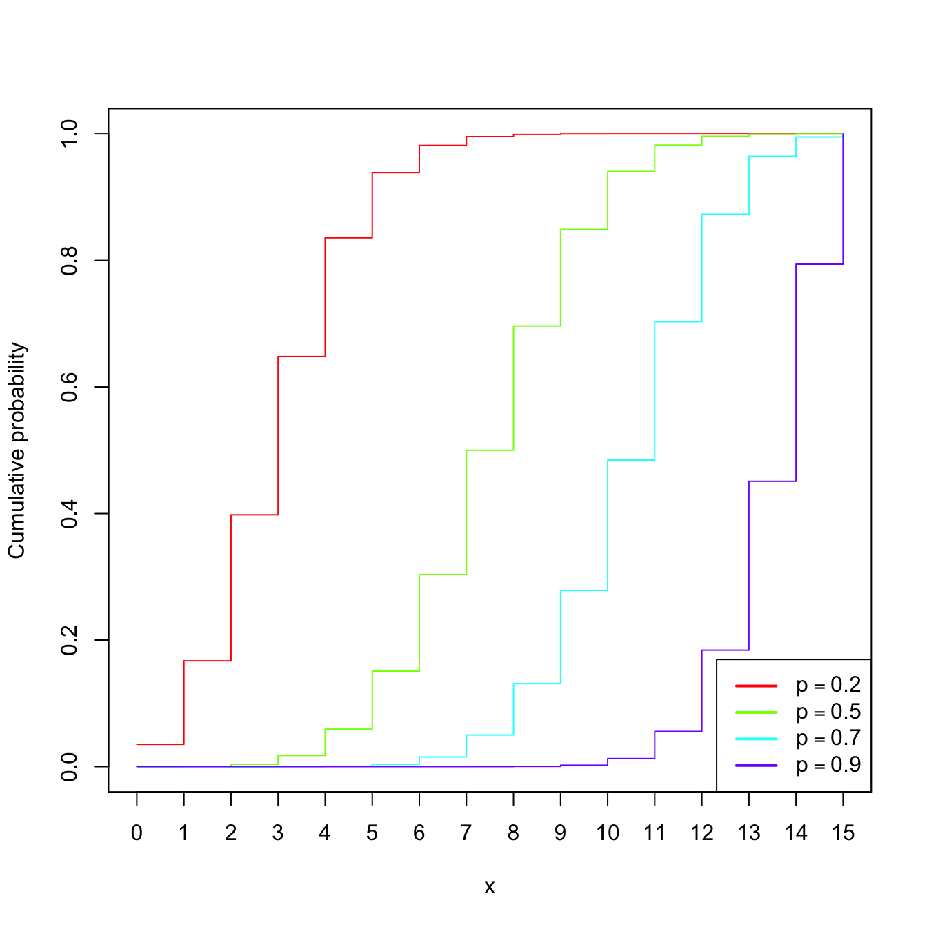
Figure 1.6: \(\mathrm{Bin}(n,p)\) pmf’s and cdf’s for size \(n=15\) and several probabilities \(p.\)

Example 1.16 (Uniform (continuous)) The random variable \(X\sim\mathcal{U}(a,b),\) \(a<b,\) is such that its pdf is

\[\begin{align*} f(x;a,b)=\begin{cases} 1/(b-a),& x\in(a,b),\\ 0,&\text{otherwise.} \end{cases} \end{align*}\]

Example 1.17 (Normal model) The random variable \(X\sim\mathcal{N}(\mu,\sigma^2)\) (notice the second argument is a variance), with mean \(\mu\in\mathbb{R}\) and standard deviation \(\sigma>0,\) has pdf

\[\begin{align*} \phi(x;\mu,\sigma^2):=\frac{1}{\sqrt{2\pi}\sigma}\exp\left\{-\frac{(x-\mu)^2}{2\sigma^2}\right\},\quad x\in\mathbb{R}. \end{align*}\]

This probability model is extremely useful to model many random variables in reality, especially those that are composed of sums of other random variables (why?).

The standard normal distribution is \(\mathcal{N}(0,1).\) A standard normal rv is typically denoted by \(Z,\) its pdf by simply \(\phi,\) and its cdf by

\[\begin{align*} \Phi(x):=\int_{-\infty}^x \phi(t)\,\mathrm{d}t. \end{align*}\]

The cdf of \(\mathcal{N}(\mu,\sigma^2)\) is \(\Phi\left(\frac{\cdot-\mu}{\sigma}\right).\)

Example 1.18 (Exponential model) The random variable \(X\sim\mathrm{Exp}(\lambda),\) \(\lambda>0\) (rate parameter), has pdf

\[\begin{align*} f(x;\lambda)=\lambda e^{-\lambda x},\quad x\in\mathbb{R}_+. \end{align*}\]

This probability model is useful to model lifetimes.

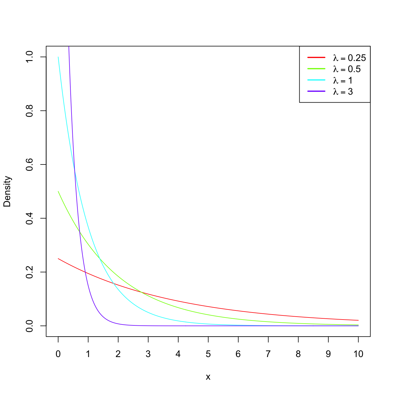
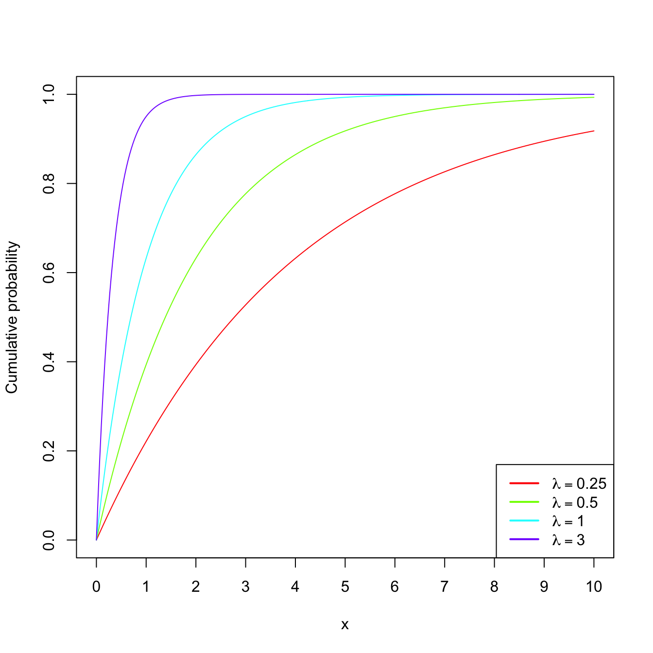
Figure 1.7: \(\mathrm{Exp}(\lambda)\) pdf’s and cdf’s for several rates \(\lambda.\)

1.2.2 Expectation and variance

Definition 1.19 (Expectation) Given a random variable \(X\sim F_X,\) its expectation \(\mathbb{E}[X]\) is defined as⁸

\[\begin{align*} \mathbb{E}[X]:=&\;\int x\,\mathrm{d}F_X(x)\\ :=&\;\begin{cases} \displaystyle\int_{\mathbb{R}} x f_X(x)\,\mathrm{d}x,&\text{ if }X\text{ is continuous,}\\ \displaystyle\sum_{\{x\in\mathbb{R}:p_X(x)>0\}} xp_X(x),&\text{ if }X\text{ is discrete.} \end{cases} \end{align*}\]

Example 1.19 Let \(X\sim \mathcal{U}(a,b).\) Then:

\[\begin{align*} \mathbb{E}[X]=&\;\int_{\mathbb{R}} x f(x;a,b)\,\mathrm{d}x=\frac{1}{b-a}\int_a^b x \,\mathrm{d}x\\ =&\;\frac{1}{b-a}\frac{b^2-a^2}{2}=\frac{a+b}{2}. \end{align*}\]

Definition 1.20 (Variance and standard deviation) The variance of the random variable \(X\) is defined as

\[\begin{align*} \mathbb{V}\mathrm{ar}[X]:=\mathbb{E}[(X-\mathbb{E}[X])^2] =\mathbb{E}[X^2]-\mathbb{E}[X]^2. \end{align*}\]

The standard deviation of \(X\) is \(\sqrt{\mathbb{V}\mathrm{ar}[X]}.\)

Example 1.20 Let \(X\sim \mathrm{Pois}(\lambda).\) Then:

\[\begin{align*} \mathbb{E}[X]=&\;\sum_{\{x\in\mathbb{R}:p(x;\lambda)>0\}} x p(x;\lambda)=\sum_{x=0}^\infty x \frac{e^{-\lambda}\lambda^x}{x!}\\ =&\;e^{-\lambda}\sum_{x=1}^\infty \frac{\lambda^x}{(x-1)!}=e^{-\lambda} \lambda \sum_{x=0}^\infty \frac{\lambda^x}{x!}\\ =&\;\lambda \end{align*}\]

using that \(e^\lambda=\sum_{x=0}^\infty \frac{\lambda^x}{x!}.\) Similarly,⁹

\[\begin{align*} \mathbb{E}[X^2]=&\;\sum_{x=0}^\infty x^2 \frac{e^{-\lambda}\lambda^x}{x!}=e^{-\lambda} \sum_{x=1}^\infty \frac{x\lambda^x}{(x-1)!}\\ =&\;e^{-\lambda} \lambda \sum_{x=0}^\infty \{1+x\}\frac{\lambda^x}{x!}=e^{-\lambda} \lambda \bigg\{e^{\lambda} + \sum_{x=1}^\infty x \frac{\lambda^x}{x!}\bigg\}\\ =&\;\lambda + e^{-\lambda} \lambda^2 \sum_{x=0}^\infty \frac{\lambda^x}{x!}=\lambda(1+\lambda). \end{align*}\]

Therefore, \(\mathbb{V}\mathrm{ar}[X]=\lambda(1+\lambda)-\lambda^2=\lambda.\)

A deeper and more general treatment of expectation and variance is given in Section 1.3.4.

1.2.3 Moment generating function

Definition 1.21 (Moment generating function) The moment generating function (mgf) of a rv \(X\) is the function

\[\begin{align*} M_X(s):=\mathbb{E}\left[e^{sX}\right], \end{align*}\]

for \(s\in(-h,h)\subset \mathbb{R},\) \(h>0,\) and such that the expectation \(\mathbb{E}\left[e^{sX}\right]\) exists. If the expectation does not exist for any neighborhood around zero, then we say that the mgf does not exist.¹⁰

Remark. In analytical terms, the mgf for a continuous random variable \(X\) is the bilateral Laplace transform of the pdf \(f_X\): \(F(s):= \int_{-\infty}^{\infty}e^{-st}f_X(t)\,\mathrm{d}t.\) If \(X>0,\) then the mgf is simply the Laplace transform of \(f_X\): \(\mathcal{L}\{f\}(s):= \int_{0}^{\infty}e^{-st}f_X(t)\,\mathrm{d}t.\)

Example 1.21 (Gamma mgf) A rv \(X\) follows a gamma distribution with shape \(\alpha\) and scale \(\beta,\) denoted as \(X\sim\Gamma(\alpha,\beta),\) if its pdf belongs to the next parametric class of densities:

\[\begin{align*} f(x;\alpha,\beta)=\frac{1}{\Gamma(\alpha)\beta^{\alpha}}x^{\alpha-1}e^{-x/\beta}, \quad x>0, \ \alpha>0,\ \beta>0, \end{align*}\]

where \(\Gamma(\alpha)\) is the gamma function, defined as

\[\begin{align*} \Gamma(\alpha):=\int_{0}^{\infty} x^{\alpha-1}e^{-x}\,\mathrm{d}x. \end{align*}\]

The gamma function satisfies the following properties:

• \(\Gamma(1)=1.\)
• \(\Gamma(\alpha)=(\alpha-1)\Gamma(\alpha-1),\) for any \(\alpha\geq 1.\)
• \(\Gamma(n)=(n-1)!,\) for any \(n\in\mathbb{N}.\)

Let us compute the mgf of \(X\):

\[\begin{align*} M_X(s)&=\mathbb{E}\left[e^{sX}\right]\\ &=\frac{1}{\Gamma(\alpha)\beta^{\alpha}}\int_{0}^{\infty} e^{sx} x^{\alpha-1}e^{-x/\beta}\,\mathrm{d}x\\ &=\frac{1}{\Gamma(\alpha)\beta^{\alpha}}\int_{0}^{\infty} x^{\alpha-1}e^{-(1/\beta -s)x}\,\mathrm{d}x\\ &=\frac{1}{\Gamma(\alpha)\beta^{\alpha}}\int_{0}^{\infty} x^{\alpha-1}e^{-x/(1/\beta -s)^{-1}}\,\mathrm{d}x. \end{align*}\]

The kernel of a pdf is the main part of the density once the constants are removed. Observe that in the integrand we have the kernel of a gamma pdf with shape \(\alpha\) and scale \((1/\beta-s)^{-1}=\beta/(1-s\beta).\) If \(s\geq 1/\beta,\) then the integral is \(\infty.\) However, if \(s<1/\beta,\) then the integral is finite, and multiplying and dividing by the adequate constants, we obtain the mgf

\[\begin{align*} M_X(s)&=\frac{1}{\beta^{\alpha}}\left(\frac{\beta}{1-s\beta}\right)^{\alpha} \int_{0}^{\infty} \frac{1}{\Gamma(\alpha)}\left(\frac{\beta}{1-s\beta}\right)^{-\alpha} x^{\alpha-1}e^{-\frac{x}{\beta/(1-s\beta)}} \,\mathrm{d}x\\ &=\frac{1}{(1-s\beta)^{\alpha}}, \quad s<1/\beta. \end{align*}\]

Recall that, since \(\beta>0,\) the mgf exists in the interval \((-h,h)\) with \(h=1/\beta;\) see Figure 1.8 for graphical insight.

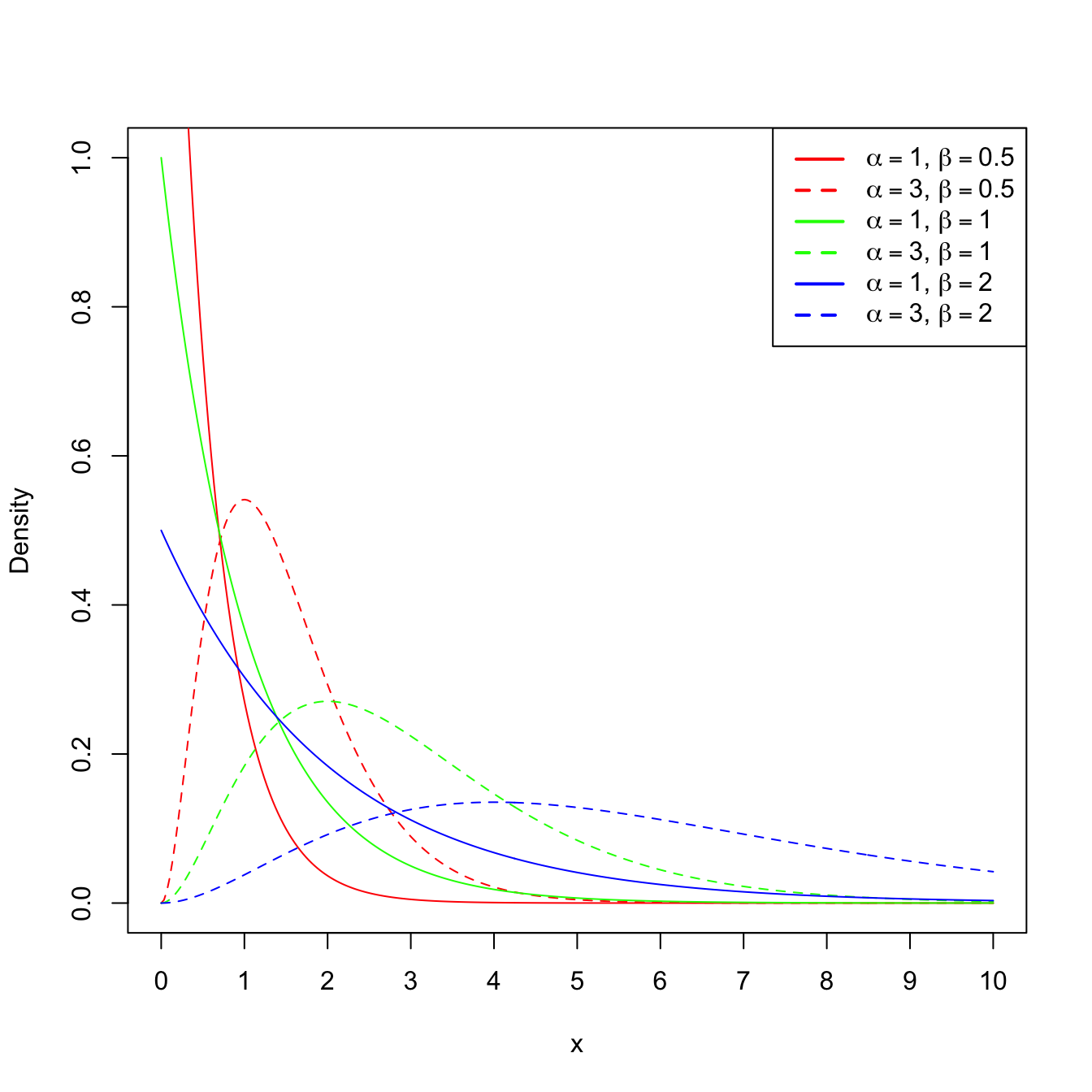
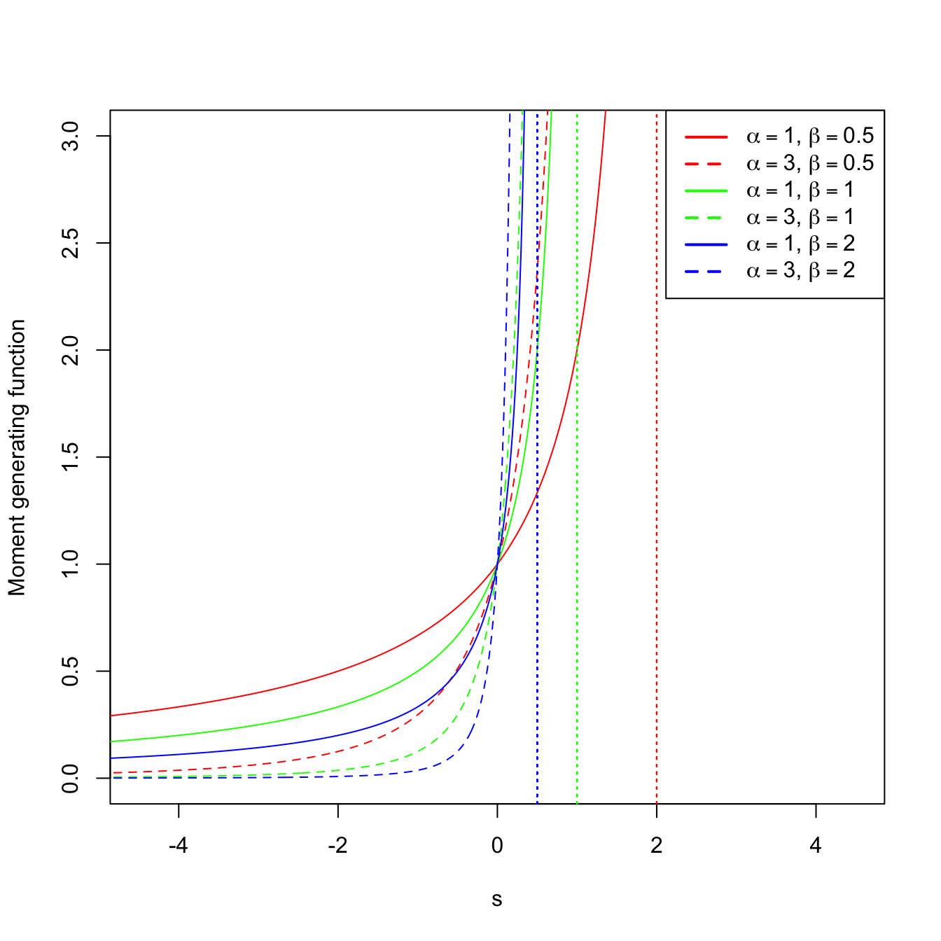
Figure 1.8: \(\Gamma(\alpha,\beta)\) pdf’s and mgf’s for several shapes \(\alpha\) and scales \(\beta.\) The dotted vertical lines represent the value \(s=1/\beta.\)

Example 1.22 (Binomial mgf) As seen in Example 1.15, the pmf of \(\mathrm{Bin}(n,p)\) is

\[\begin{align*} p(x;n,p)=\binom{n}{x} p^x (1-p)^{n-x}, \quad x=0,1,2,\ldots \end{align*}\]

Let us compute its mgf:

\[\begin{align*} M_X(s)=\sum_{x=0}^{\infty} e^{sx}\binom{n}{x} p^x (1-p)^{n-x}=\sum_{x=0}^{\infty} \binom{n}{x} (pe^s)^x (1-p)^{n-x}. \end{align*}\]

By Newton’s generalized binomial theorem, we know that¹¹

\[\begin{align} (a+b)^r =\sum_{x=0}^{\infty} \binom{r}{x} a^x b^{r-x},\quad a,b,r\in\mathbb{R},\tag{1.3} \end{align}\]

and therefore the mgf is

\[\begin{align*} M_X(s)=(pe^s+1-p)^n, \quad \forall s\in\mathbb{R}. \end{align*}\]

The mgf is shown in Figure 1.9, which displays how \(M_X\) is continuous despite the pmf being discrete.

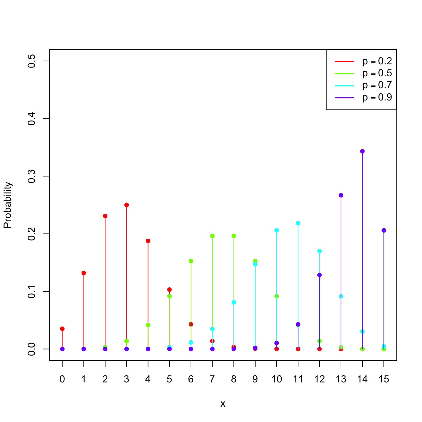
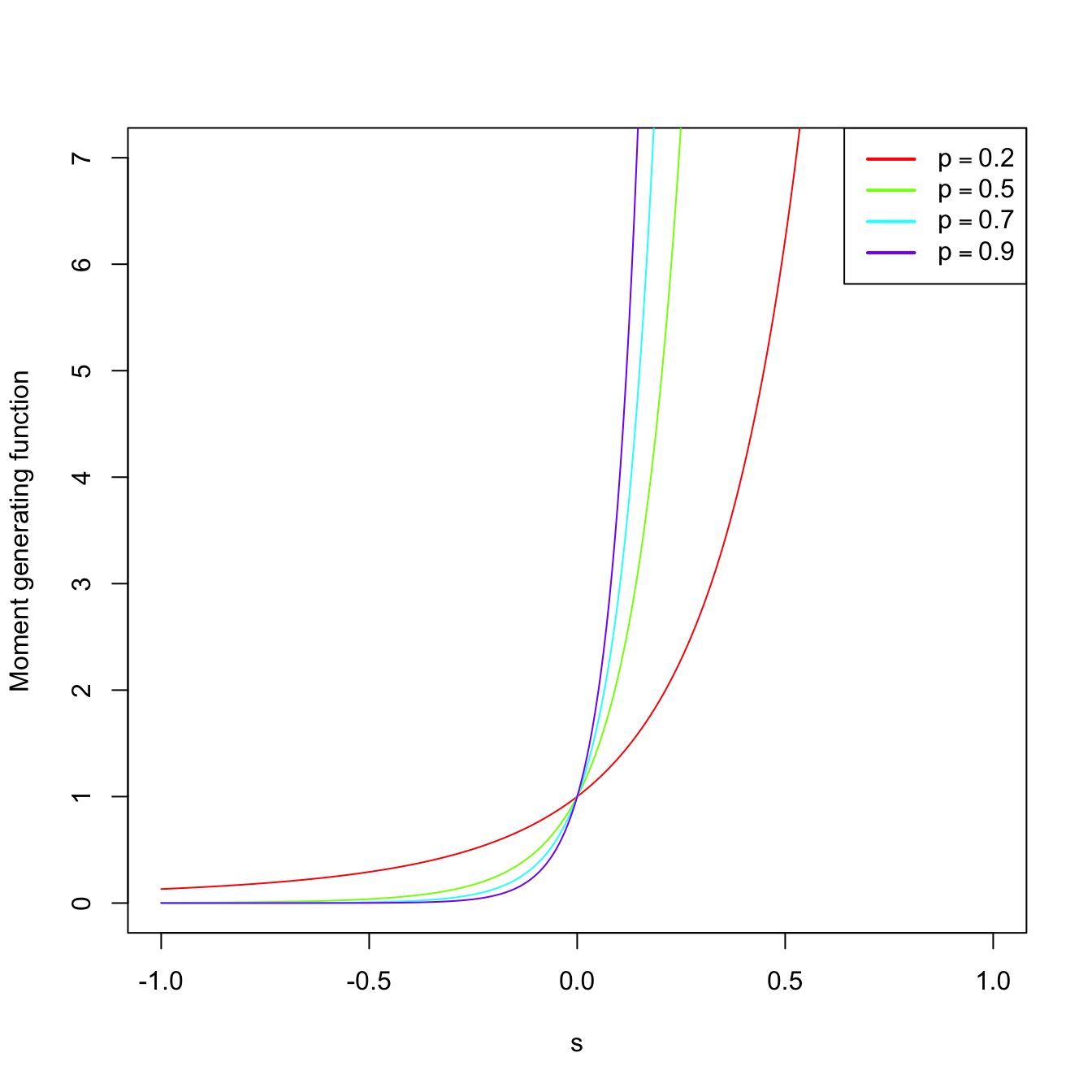
Figure 1.9: \(\mathrm{Bin}(n,p)\) pmf’s and mgf’s for size \(n=15\) and several probabilities \(p.\)

The following theorem says that, as its name indicates, the mgf of a rv \(X\) indeed generates the raw moments of \(X\) (that is, the moments centered about \(0\)).

Theorem 1.1 (Moment generation by the mgf) Let \(X\) be a rv with mgf \(M_X.\) Then,

\[\begin{align*} \mathbb{E}[X^n]=M_X^{(n)}(0), \end{align*}\]

where \(M_X^{(n)}(0)\) denotes the \(n\)-th derivative of the mgf with respect to \(s,\) evaluated at \(s=0.\)

Example 1.23 Let us compute the expectation and variance of \(X\sim\Gamma(\alpha,\beta).\) Using Theorem 1.1 and Example 1.21,

\[\begin{align*} \mathbb{E}[X]=M_X^{(1)}(0)=\left.\frac{\mathrm{d}}{\mathrm{d} s}\frac{1}{(1-s\beta)^{\alpha}}\right\vert_{s=0}=\left.\frac{\alpha\beta}{(1-s\beta)^{\alpha+1}}\right\vert_{s=0}=\alpha\beta. \end{align*}\]

Analogously,

\[\begin{align*} \mathbb{E}[X^2]=M_X^{(2)}(0)=\left.\frac{\mathrm{d}^2}{\mathrm{d} s^2}\frac{1}{(1-s\beta)^{\alpha}}\right\vert_{s=0}=\left. \frac{\alpha(\alpha+1)\beta^2}{(1-s\beta)^{\alpha+2}}\right\vert_{s=0}=\alpha(\alpha+1)\beta^2. \end{align*}\]

Therefore,

\[\begin{align*} \mathbb{V}\mathrm{ar}[X]=\mathbb{E}[X^2]-\mathbb{E}[X]^2=\alpha(\alpha+1)\beta^2-\alpha^2\beta^2=\alpha\beta^2. \end{align*}\]

The result below is important because it shows that the distribution of a rv is determined from its mgf.

Theorem 1.2 (Uniqueness of the mgf) Let \(X\) and \(Y\) two rv’s with mgf’s \(M_X\) and \(M_Y,\) respectively. If

\[\begin{align*} M_X(s)=M_Y(s), \quad \forall s\in (-h,h), \end{align*}\]

then the distributions of \(X\) and \(Y\) are the same.

The following properties of the mgf are very useful to manipulate mgf’s of linear combinations of independent random variables.

Proposition 1.5 (Properties of the mgf) The mgf satisfies the following properties:

1. Let \(X\) be a rv with mgf \(M_X.\) Define the rv \[\begin{align*} Y=aX+b, \quad a,b\in \mathbb{R}, \ a\neq 0. \end{align*}\] Then, the mgf of the new rv \(Y\) is \[\begin{align*} M_Y(s)=e^{sb}M_X(as). \end{align*}\]

2. Let \(X_1,\ldots,X_n\) be independent¹² rv’s with mgf’s \(M_{X_1},\ldots,M_{X_n},\) respectively. Let be the rv \[\begin{align*} Y=X_1+\cdots+X_n. \end{align*}\] Then, its mgf is given by \[\begin{align*} M_Y(s)=\prod_{i=1}^n M_{X_i}(s). \end{align*}\]

Proof (Proof of Proposition 1.5). In order to see i, observe that

\[\begin{align*} M_Y(s)&=\mathbb{E}\left[e^{sY}\right]=\mathbb{E}\left[e^{s(aX+b)}\right]=\mathbb{E}\left[e^{saX}e^{sb}\right]\\ &=e^{sb}\mathbb{E}\left[e^{saX}\right]=e^{sb}M_X(as). \end{align*}\]

To check ii, consider

\[\begin{align*} M_Y(s)&=\mathbb{E}\left[e^{sY}\right]=\mathbb{E}\left[e^{s\sum_{i=1}^n X_i}\right]=\mathbb{E}\left[e^{sX_1}\cdots e^{sX_n}\right]\\ &=\mathbb{E}\left[e^{sX_1}\right]\cdots \mathbb{E}\left[e^{sX_n}\right]=\prod_{i=1}^n M_{X_i}(s). \end{align*}\]

The equality \(\mathbb{E}\left[e^{sX_1}\cdots e^{sX_n}\right]=\mathbb{E}\left[e^{sX_1}\right]\cdots \mathbb{E}\left[e^{sX_n}\right]\) is only satisfied because of the independence of \(X_1,\ldots,X_n.\)

The next theorem is very useful for proving convergence in distribution¹³ of random variables by employing a simple-to-use function such as the mgf. For example, the central limit theorem, a cornerstone result in statistical inference, can be easily proved using Theorem 1.3.

Theorem 1.3 (Convergence of the mgf) Assume that \(X_n,\) \(n=1,2,\ldots\) is a sequence of rv’s with respective mgf’s \(M_{X_n},\) \(n\geq 1.\) Assume in addition that, for all \(s\in(-h,h)\) with \(h>0,\) it holds

\[\begin{align*} \lim_{n\to\infty} M_{X_n}(s)=M_X(s), \end{align*}\]

where \(M_X\) is a mgf. Then there exists a unique cdf \(F_X\) whose moments are determined by \(M_X\) and, for all \(x\) where \(F_X(x)\) is continuous, it holds

\[\begin{align*} \lim_{n\to\infty} F_{X_n}(x)=F_X(x). \end{align*}\]

That is, the convergence of mgf’s implies the convergence of cdf’s.

1.3 Random vectors

A random vector is just a collection of random variables generated by the same measurable space \((\Omega,\mathcal{A})\) associated to an experiment \(\xi.\) Before formally defining them, we need to generalize Definition 1.4.

Definition 1.22 (Borel \(\sigma\)-algebra in \(\mathbb{R}^p\)) Let \(\Omega=\mathbb{R}^p,\) \(p\geq 1.\) Consider the collection of hyperrectangles

\[\begin{align*} \mathcal{I}^p:=\{(-\infty,a_1]\times\stackrel{p}{\cdots} \times(-\infty,a_p]: a_1,\ldots,a_p\in \mathbb{R}\}. \end{align*}\]

The Borel \(\sigma\)-algebra in \(\mathbb{R^p}\), denoted by \(\mathcal{B}^p,\) is defined as the smallest \(\sigma\)-algebra that contains \(\mathcal{I}^p.\)

Definition 1.23 (Random vector) Let \((\Omega,\mathcal{A})\) be measurable space. Let \(\mathcal{B}^p\) be the Borel \(\sigma\)-algebra over \(\mathbb{R}^p.\) A random vector is a mapping \(\boldsymbol{X}:\Omega\rightarrow \mathbb{R}^p\) that is measurable, that is, that verifies

\[\begin{align*} \forall B\in\mathcal{B}^p, \quad \boldsymbol{X}^{-1}(B)\in\mathcal{A}, \end{align*}\]

with \(\boldsymbol{X}^{-1}(B)=\{\omega\in\Omega: \boldsymbol{X}(\omega)\in B\}.\)

It is clear that the above generalizes Definition 1.13, which follows for \(p=1.\) It is nevertheless simpler to think about random vectors in terms of the following characterization, which states that a random vector is indeed just a collection of random variables.

Proposition 1.6 Given a measurable space \((\Omega,\mathcal{A}),\) a mapping \(\boldsymbol{X}:\Omega\rightarrow \mathbb{R}^p\) defined as \(\boldsymbol{X}(\omega)=(X_1(\omega),\ldots,X_p(\omega))^\top\) is a random vector if and only if \(X_1,\ldots,X_p:\Omega\rightarrow \mathbb{R}\) are random variables in \((\Omega,\mathcal{A}).\)¹⁴

Example 1.24 Let \(\xi=\) “Roll a dice \(10\) times”. Then, \(\#\Omega=6^{10}.\) We can define the random vector \(\boldsymbol{X}(\omega)=(X_1(\omega),X_2(\omega))^\top\) where \(X_1(\omega)=\) “Number of \(5\)’s in \(\omega\)” and \(X_2(\omega)=\) “Number of \(3\)’s in \(\omega\)” (\(\omega\) is the random output of \(\xi,\) i.e., the information of the obtained \(10\) sides of the rolled dice).

It can be seen that \(\boldsymbol{X}\) is a random vector, comprised by the random variables \(X_1\) and \(X_2,\) with respect to the measurable space \((\Omega,\mathcal{P}(\Omega)).\)

As a random variable does, a random vector \(\boldsymbol{X}\) also induces a probability \(\mathbb{P}_{\boldsymbol{X}}\) over \((\mathbb{R}^p,\mathcal{B}^p)\) from a probability \(\mathbb{P}\) in \((\Omega,\mathcal{A}).\) The following is an immediate generalization of Definition 1.14.

Definition 1.24 (Induced probability of a random vector) Let \(\mathcal{B}^p\) be the Borel \(\sigma\)-algebra over \(\mathbb{R}^p.\) The induced probability of the random vector \(\boldsymbol{X}\) is the function \(\mathbb{P}_{\boldsymbol{X}}:\mathcal{B}^p\rightarrow \mathbb{R}^p\) defined as

\[\begin{align*} \mathbb{P}_{\boldsymbol{X}}(B):=\mathbb{P}(\boldsymbol{X}^{-1}(B)), \quad \forall B\in \mathcal{B}^p. \end{align*}\]

Example 1.25 In Example 1.24, a probability for \(\xi\) that is compatible with common belief is \(\mathbb{P}(\{\omega\})=6^{-10},\) \(\forall\omega\in\Omega.\) With this probability, we have a probability space \((\Omega,\mathcal{A},\mathbb{P}).\) The induced probability \(\mathbb{P}_{\boldsymbol{X}}\) could be worked out from this probability.

In the previous example, the induced probability by \(\boldsymbol{X}\) can be computed following Definition 1.24, thus generating the probability space \((\mathbb{R}^2,\mathcal{B}^2,\mathbb{P}_{\boldsymbol{X}}).\) However, as indicated with random variables, we will not need to do this in practice: we will directly specify \(\mathbb{P}_{\boldsymbol{X}}\) via probability models, in this case for random vectors, and forget about the conceptual pillars on which \(\mathbb{P}_{\boldsymbol{X}}\) is built (the random experiment \(\xi\) and the probability space \((\Omega,\mathcal{A},\mathbb{P})\)). Again, for introducing probability models, we need to distinguish first among the two most common types of random vectors: discrete and continuous.

1.3.1 Types of random vectors

Definition 1.25 (Joint cdf for random vectors) The joint cumulative distribution function (joint cdf or simply cdf) of a random vector \(\boldsymbol{X}\) is the function \(F_{\boldsymbol{X}}:\mathbb{R}^p\rightarrow [0,1]\) defined as

\[\begin{align*} F_{\boldsymbol{X}}(\boldsymbol{x}):=\mathbb{P}_{\boldsymbol{X}}((-\infty,x_1]\times\stackrel{p}{\cdots}\times(-\infty,x_p]), \quad \forall \boldsymbol{x}=(\boldsymbol{x}_1,\ldots, \boldsymbol{x}_p)^\top\in \mathbb{R}^p. \end{align*}\]

We will denote \(\mathbb{P}(\boldsymbol{X}\leq \boldsymbol{x}):=\mathbb{P}_{\boldsymbol{X}}((-\infty,x_1]\times\stackrel{p}{\cdots}\times(-\infty,x_p])\) for simplicity.

Remark. The notation \(\mathbb{P}(\boldsymbol{X}\leq \boldsymbol{x})\) equivalently means

\[\begin{align*} \mathbb{P}(\boldsymbol{X}\leq \boldsymbol{x})&=\mathbb{P}(X_1\leq x_1,\ldots,X_p\leq x_p)\\ &=\mathbb{P}(\{X_1\leq x_1\}\cap \ldots\cap \{X_p\leq x_p\}). \end{align*}\]

Proposition 1.7 (Properties of the joint cdf)

1. The cdf is monotonically non-decreasing, in each component, that is, \[\begin{align*} x_i<y_i \implies F_{\boldsymbol{X}}(\boldsymbol{x})\leq F_{\boldsymbol{X}}(\boldsymbol{y}),\quad \text{for all }i=1,\ldots,p. \end{align*}\]

2. \(\lim_{x_i\to-\infty} F(\boldsymbol{x})=0\) for all \(i=1,\ldots,p.\)

3. \(\lim_{\boldsymbol{x}\to+\boldsymbol{\infty}} F(\boldsymbol{x})=1.\)

4. \(F_{\boldsymbol{X}}\) is right-continuous.¹⁵

Definition 1.26 (Discrete random vector) A random vector \(\boldsymbol{X}\) is discrete if its range (or image set) \(R_{\boldsymbol{X}}:=\{\boldsymbol{x}\in \mathbb{R}^p: \boldsymbol{x}=\boldsymbol{X}(\omega)\ \text{for some} \ \omega\in \Omega\}\) is finite or countable.

Definition 1.27 (Joint pmf for random vectors) The probability mass function (pmf) of a discrete random vector \(\boldsymbol{X}\) is the function \(p_{\boldsymbol{X}}:\mathbb{R}^p\rightarrow [0,1]\) defined as

\[\begin{align*} p_{\boldsymbol{X}}(\boldsymbol{x}):=\mathbb{P}_{\boldsymbol{X}}(\{\boldsymbol{x}\}), \quad \forall \boldsymbol{x}\in \mathbb{R}^p. \end{align*}\]

The notation \(\mathbb{P}(\boldsymbol{X}=\boldsymbol{x}):=p_{\boldsymbol{X}}(\boldsymbol{x})\) is also often employed.

Definition 1.28 (Continuous random vector) A continuous random vector \(\boldsymbol{X}\) (also denoted absolutely continuous) is the one whose cdf \(F_{\boldsymbol{X}}\) is expressible as

\[\begin{align*} F_{\boldsymbol{X}}(\boldsymbol{x})&=\int_{-\infty}^{x_1}\cdots\int_{-\infty}^{x_p} f_{\boldsymbol{X}}(t_1,\ldots,t_p)\,\mathrm{d}t_p\cdots\mathrm{d}t_1,\quad\forall \boldsymbol{x}\in\mathbb{R}^p, \end{align*}\]

where \(f_{\boldsymbol{X}}:\mathbb{R}^p\rightarrow[0,\infty).\) The function \(f_{\boldsymbol{X}}\) is the joint probability density function (joint pdf or simply pdf) of \(\boldsymbol{X}.\)

Proposition 1.8 (Properties of the joint pdf)

1. \(\frac{\partial^p}{\partial x_1\cdots\partial x_p}F_{\boldsymbol{X}}(\boldsymbol{x})=f_{\boldsymbol{X}}(\boldsymbol{x})\) for almost all \(\boldsymbol{x}\in\mathbb{R}^p.\)¹⁶

2. \(f\) is nonnegative and such that \[\begin{align*} \int_{-\infty}^{\infty}\cdots\int_{-\infty}^{\infty} f_{\boldsymbol{X}}(t_1,\ldots,t_p)\,\mathrm{d}t_p\cdots\mathrm{d}t_1=\int_{\mathbb{R}^p} f_{\boldsymbol{X}}(\boldsymbol{t})\,\mathrm{d}\boldsymbol{t}=1. \end{align*}\]

3. For \(A\in\mathcal{B}^p,\) \(\mathbb{P}(\boldsymbol{X}\in A)=\int_{A} f_{\boldsymbol{X}}(\boldsymbol{t})\,\mathrm{d}\boldsymbol{t}.\)¹⁷

Remark. As for random variables, recall that the cdf accumulates probability irrespective of the type of the random vector. Probability assignment to specific values of \(\boldsymbol{X}\) is a type-dependent operation.

Example 1.26 (Uniform random vector) Take \(\boldsymbol{X}\sim\mathcal{U}([0,1]\times[0,2]).\) The joint pdf of \(\boldsymbol{X}\) is

\[\begin{align*} f(x_1,x_2)=\begin{cases} 1/2,&(x_1,x_2)^\top\in[0,1]\times[0,2],\\ 0,&\text{otherwise.} \end{cases} \end{align*}\]

The joint cdf of \(\boldsymbol{X}\) is

\[\begin{align*} F(x_1,x_2)=\int_{-\infty}^{x_1}\int_{-\infty}^{x_2}f(t_1,t_2)\,\mathrm{d}t_2\,\mathrm{d}t_1. \end{align*}\]

Therefore, carefully taking into account the definition of \(f,\) we get

\[\begin{align*} F(x_1,x_2)=\begin{cases} 0,&x_1<0\text{ or }x_2<0,\\ x_1,&0\leq x_1\leq 1,x_2>2,\\ (x_1x_2)/2,&0\leq x_1\leq 1,0\leq x_2\leq 2,\\ x_2/2,&x_1> 1,0\leq x_2\leq 2,\\ 1,&x_1>1,x_2>2. \end{cases} \end{align*}\]

Example 1.27 (A discrete random vector) Let \(\boldsymbol{X}=(X_1,X_2)^\top,\) where \(X_1\sim\mathcal{U}(\{1,2,3\})\) and \(X_2\sim \mathrm{Bin}(1, 2/3)\) (both variables are independent of each other). This means that:

• \(\mathbb{P}(X_1=x)=1/3,\) for \(x=1,2,3\) (and zero otherwise).
• \(\mathbb{P}(X_2=1)=2/3\) and \(\mathbb{P}(X_2=0)=1/3\) (and zero otherwise).
• \(\mathbb{P}(X_1=x_1,X_2=x_2)=\mathbb{P}(X_1=x_1)\mathbb{P}(X_2=x_2).\)
• The atoms of \(\boldsymbol{X}\) are \(\{(1,0),(2,0),(3,0),(1,1),(2,1),(3,1)\}.\)

Let us compute the cdf \(F\) evaluated at \((5/2,1/2)\):

\[\begin{align*} F(5/2,1/2)&=\mathbb{P}(X_1\leq 5/2,X_2\leq 1/2)\\ &=\mathbb{P}(X_1=1,X_2=0)+\mathbb{P}(X_1=2,X_2=0)\\ &=(1/3)^2 + (1/3)^2\\ &=2/9. \end{align*}\]

1.3.2 Marginal distributions

The joint cdf/pdf/pmf characterize the joint random behavior of \(\boldsymbol{X}.\) What about the behavior of each component of \(\boldsymbol{X}\)?

Definition 1.29 (Marginal cdf) The \(i\)-th marginal cumulative distribution function (marginal cdf) of a random vector \(\boldsymbol{X}\) is defined as

\[\begin{align*} F_{X_i}(x_i):=&\;F_{\boldsymbol{X}}(\infty,\ldots,\infty,x_i,\infty,\ldots,\infty)\\ =&\;\mathbb{P}(X_1\leq \infty,\ldots,X_i\leq x_i,\ldots,X_p\leq \infty)\\ =&\;\mathbb{P}(X_i\leq x_i). \end{align*}\]

Definition 1.30 (Marginal pdf) The \(i\)-th marginal probability density function (marginal pdf) of a random vector \(\boldsymbol{X}\) is defined as

\[\begin{align*} f_{X_i}(x_i):=&\;\frac{\partial}{\partial x_i}F_{X_i}(x_i)\\ =&\;\int_{-\infty}^{\infty}\stackrel{p-1}{\cdots}\int_{-\infty}^{\infty} f_{\boldsymbol{X}}(x_1,\ldots,x_i,\ldots,x_p)\,\mathrm{d}x_p\stackrel{p-1}{\cdots}\mathrm{d}x_1\\ =&\;\int_{\mathbb{R}^{p-1}} f_{\boldsymbol{X}}(\boldsymbol{x})\,\mathrm{d}\boldsymbol{x}_{-i}, \end{align*}\]

where \(\boldsymbol{x}_{-i}=(x_1,\ldots,x_{i-1},x_{i+1},\ldots,x_p)^\top\) is the vector \(\boldsymbol{x}\) without the \(i\)-th entry.

Definition 1.31 (Marginal pmf) The \(i\)-th marginal probability mass function (marginal pmf) of a random vector \(\boldsymbol{X}\) is defined as

\[\begin{align*} p_{X_i}(x_i):=\sum_{\{x_1\in\mathbb{R}:p_{X_1}(x_1)>0\}}\stackrel{p-1}{\cdots}\sum_{\{x_p\in\mathbb{R}:p_{X_p}(x_p)>0\}} p_{\boldsymbol{X}}(x_1,\ldots,x_i,\ldots,x_p). \end{align*}\]

Getting marginal cdfs/pdfs/pmfs from joint cdf/pdf/pmf is always possible. What about the converse?

1.3.3 Conditional distributions

Just as the cdf/pdf/pmf of a random vector allows us to easily work with the probability function \(\mathbb{P}\) of a probability space \((\Omega,\mathcal{A},\mathbb{P}),\) the conditional cdf/pdf/pmf of a random variable¹⁸ given another will serve to work with the conditional probability as defined in Definition 1.11. To help out with the intuition of the following definitions, recall that we can re-express (1.1) as

\[\begin{align*} \mathbb{P}(A\textbf{ conditioned to } B):=\frac{\mathbb{P}(\text{$A$ and $B$ } \textbf{jointly})}{\mathbb{P}(B\textbf{ alone})}. \end{align*}\]

Conditional distributions allow answering the next question: if we have a random vector \((X_1,X_2)^\top,\) what can we say about the randomness of \(X_2 \mid X_1=x_1\)? Conditional distributions are type-dependent; we see them next for continuous and discrete rv’s.

Definition 1.32 (Conditional pdf and cdf for a continuous random vector) Given a continuous random vector \(\boldsymbol{X}=(X_1,X_2)^\top\) with joint pdf \(f_{\boldsymbol{X}},\) the conditional pdf of \(X_1\) given \(X_2=x_2\), \(f_{X_2}(x_2)>0,\) is the pdf of the continuous random variable \(X_1 \mid X_2=x_2\):

\[\begin{align} f_{X_1 \mid X_2=x_2}(x_1):=\frac{f_{\boldsymbol{X}}(x_1,x_2)}{f_{X_2}(x_2)}.\tag{1.4} \end{align}\]

The conditional cdf of \(X_1\) given \(X_2=x_2\) is

\[\begin{align*} F_{X_1 \mid X_2=x_2}(x_1)=\int_{-\infty}^{x_1}f_{X_1 \mid X_2=x_2}(t)\mathrm{d}t. \end{align*}\]

Definition 1.33 (Conditional pmf and cdf for a discrete random vector) Given a discrete random vector \(\boldsymbol{X}=(X_1,X_2)^\top\) with joint pmf \(p_{\boldsymbol{X}},\) the conditional pmf of \(X_1\) given \(X_2=x_2\), \(p_{X_2}(x_2)>0,\) is the pmf of the discrete random variable \(X_1 \mid X_2=x_2\):

\[\begin{align} p_{X_1 \mid X_2=x_2}(x_1):=\frac{p_{\boldsymbol{X}}(x_1,x_2)}{p_{X_2}(x_2)}.\tag{1.5} \end{align}\]

The conditional cdf of \(X_1\) given \(X_2=x_2\) is

\[\begin{align*} F_{X_1 \mid X_2=x_2}(x_1)=\sum_{\{x\in\mathbb{R}:p_{X_1 \mid X_2=x_2}(x)>0,\,x\leq x_1\}}p_{X_1 \mid X_2=x_2}(x). \end{align*}\]

Remark. Recall the similarities of (1.4) and (1.5) with (1.1).

Remark. Recall that the conditional pdf/pmf/cdf of \(X_1\) given \(X_2=x_2\) is a family of functions, each with argument \(x_1,\) that is indexed by the values \(X_2=x_2.\)

The conditional cdf/pdf/pmf of \(X_2\) given \(X_1=x_1\) are defined analogously to Definitions 1.32 and 1.33. The previous definitions can be extended to account for conditioning of one random vector onto another with similar constructions.

Remark. Mixed types of conditioning, such as “discrete\(\mid\)continuous” or “continuous\(\mid\)discrete” are possible, but require the consideration of singular random vectors. These types of random vectors are neither continuous nor discrete, but a mix of them, and are more complex.

Once we have the notion of joint, marginal, and conditional distributions, we are in position of defining when two random variables are independent between them. This will resemble Definition 1.12. Indeed, we can define the concept of independence from different angles, as collected in the following definition.

Definition 1.34 (Independent random variables) Two random variables \(X_1\) and \(X_2\) are independent if and only if

\[\begin{align*} F_{\boldsymbol{X}}(x_1,x_2)=F_{X_1}(x_1)F_{X_2}(x_2),\quad \forall (x_1,x_2)^\top\in\mathbb{R}^2, \end{align*}\]

where \(\boldsymbol{X} =(X_1,X_2)^\top.\) Equivalently:

1. If \(\boldsymbol{X}\) is continuous, \(X_1\) and \(X_2\) are independent if and only if \[\begin{align} f_{\boldsymbol{X}}(x_1,x_2)=f_{X_1}(x_1)f_{X_2}(x_2),\quad \forall (x_1,x_2)^\top\in\mathbb{R}^2.\tag{1.6} \end{align}\]
2. If \(\boldsymbol{X}\) is discrete, \(X_1\) and \(X_2\) are independent if and only if \[\begin{align} p_{\boldsymbol{X}}(x_1,x_2)=p_{X_1}(x_1)p_{X_2}(x_2),\quad \forall (x_1,x_2)^\top\in\mathbb{R}^2.\tag{1.7} \end{align}\]

In virtue of the conditional pdf/pmf, the following are equivalent definitions to (1.6) and (1.7):

1. If \(\boldsymbol{X}\) is continuous, \(X_1\) and \(X_2\) are independent if and only if \[\begin{align*} f_{X_1 \mid X_2=x_2}(x_1)=f_{X_1}(x_1),\quad \forall (x_1,x_2)^\top\in\mathbb{R}^2. \end{align*}\]
2. If \(\boldsymbol{X}\) is discrete, \(X_1\) and \(X_2\) are independent if and only if \[\begin{align*} p_{X_1 \mid X_2=x_2}(x_1)=p_{X_1}(x_1),\quad \forall (x_1,x_2)^\top\in\mathbb{R}^2. \end{align*}\]

Definition 1.34 is also immediately applicable to collections of \(p>2\) random variables. Indeed, the random variables in \(\boldsymbol{X}=(X_1,\ldots,X_p)^\top\) are (mutually) independent if and only if \[\begin{align} F_{\boldsymbol{X}}(\boldsymbol{x})=\prod_{i=1}^pF_{X_i}(x_i),\quad \forall \boldsymbol{x}\in\mathbb{R}^p. \tag{1.8} \end{align}\]

If \(\boldsymbol{X}\) is continuous/discrete, then (1.8) is equivalent to the factorization of the joint pdf/pmf into its marginals.

1.3.4 Expectation and variance-covariance matrix

Definition 1.35 (Expectation of a random vector) Given a random vector \(\boldsymbol{X}\sim F_{\boldsymbol{X}}\) in \(\mathbb{R}^p,\) its expectation \(\mathbb{E}[\boldsymbol{X}],\) a vector in \(\mathbb{R}^p,\) is defined as

\[\begin{align*} \mathbb{E}[\boldsymbol{X}]:=&\;\int \boldsymbol{x}\,\mathrm{d}F_{\boldsymbol{X}}(\boldsymbol{x})\\ :=&\;\begin{cases} \displaystyle\int_{\mathbb{R}^p} \boldsymbol{x} f_{\boldsymbol{X}}(\boldsymbol{x})\,\mathrm{d}\boldsymbol{X},&\text{ if }\boldsymbol{X}\text{ is continuous,}\\ \displaystyle\sum_{\{\boldsymbol{x}\in\mathbb{R}^p:p_{\boldsymbol{X}}(\boldsymbol{x})>0\}} \boldsymbol{x}p_{\boldsymbol{X}}(\boldsymbol{x}),&\text{ if }\boldsymbol{X}\text{ is discrete.} \end{cases} \end{align*}\]

Recall that the expectation \(\mathbb{E}[\boldsymbol{X}]\) is just the vector of marginal expectations \((\mathbb{E}[X_1],\ldots,\mathbb{E}[X_p])^\top.\) That is, if \(\boldsymbol{X}\) is continuous, then

\[\begin{align*} \mathbb{E}[\boldsymbol{X}]=&\;(\mathbb{E}[X_1],\ldots,\mathbb{E}[X_p])^\top\\ =&\;\left(\int_{\mathbb{R}} x_1 f_{X_1}(x_1)\,\mathrm{d}x_1,\ldots, \int_{\mathbb{R}} x_p f_{X_p}(x_p)\,\mathrm{d}x_p\right)^\top. \end{align*}\]

Example 1.28 Let \(\boldsymbol{X}=(X_1,X_2)^\top\) be a random vector with joint pdf \(f(x,y)=e^{-(x+y)}1_{\{x,y>0\}}\) (check that it integrates one). Then:

\[\begin{align*} \mathbb{E}[\boldsymbol{X}]=&\;\int_{\mathbb{R}^2} (x,y)^\top f(x,y)\,\mathrm{d}x\,\mathrm{d}y\\ =&\;\left(\int_{\mathbb{R}^2} x f(x,y)\,\mathrm{d}x\,\mathrm{d}y,\int_{\mathbb{R}^2} y f(x,y)\,\mathrm{d}x\,\mathrm{d}y\right)^\top\\ =&\;\left(\int_{0}^\infty\int_{0}^\infty x e^{-(x+y)}\,\mathrm{d}x\,\mathrm{d}y,\int_{0}^\infty\int_{0}^\infty y e^{-(x+y)}\,\mathrm{d}x\,\mathrm{d}y\right)^\top\\ =&\;\left(\int_{0}^\infty x e^{-x}\,\mathrm{d}x,\int_{0}^\infty y e^{-y}\mathrm{d} y\right)^\top\\ =&\;\left(1,1\right)^\top. \end{align*}\]

Example 1.29 Let \(\boldsymbol{X}=(X_1,X_2)^\top\) be a random vector with joint pmf given by

\[\begin{align*} p(x,y)=\begin{cases} 3/8,&\text{if }(x,y)=(0,1),\\ 1/8,&\text{if }(x,y)=(2,0),\\ 1/2,&\text{if }(x,y)=(1,-1),\\ 0,&\text{otherwise.} \end{cases} \end{align*}\]

Then:

\[\begin{align*} \mathbb{E}[\boldsymbol{X}]=&\;\sum_{\{(x,y)^\top\in\mathbb{R}^2:p(x,y)>0\}} (x,y)^\top p(x,y)\\ =&\;(0,1)^\top3/8+(2,0)^\top1/8+(1,-1)^\top1/2\\ =&\;(3/4,-1/8)^\top. \end{align*}\]

Since the expectation is defined as a (finite or infinite) sum, it is clearly a linear operator.

Proposition 1.9 If \(\boldsymbol{X}\) is a random vector in \(\mathbb{R}^p,\) then

\[\begin{align*} \mathbb{E}[\boldsymbol{A} \boldsymbol{X} + \boldsymbol{b}]=\boldsymbol{A} \mathbb{E}[\boldsymbol{X}] + \boldsymbol{b} \end{align*}\]

for any \(q\times p\) matrix \(\boldsymbol{A}\) and any \(\boldsymbol{b}\in\mathbb{R}^q.\)

Computing the expectation of a function \(g(\boldsymbol{X})\) of a random vector \(\boldsymbol{X}\) is very easy thanks to the following “law”, which affords the statistician the computation of \(\mathbb{E}[g(\boldsymbol{X})]\) only using the distribution of \(\boldsymbol{X}\) and not the distribution of \(g(\boldsymbol{X})\) (which would need to be derived in a more complicated form; see Section 1.4).

Proposition 1.10 (Law of the unconscious statistician) If \(\boldsymbol{X}\sim F_{\boldsymbol{X}}\) in \(\mathbb{R}^p\) and \(g:\mathbb{R}^p\rightarrow\mathbb{R}^q,\) then

\[\begin{align*} \mathbb{E}[g(\boldsymbol{X})]=\int g(\boldsymbol{x})\,\mathrm{d}F_{\boldsymbol{X}}(\boldsymbol{x}). \end{align*}\]

Example 1.30 What is the expectation of \(X_1X_2,\) given that \(\boldsymbol{X}\sim \mathcal{U}([0,1]\times[0,2])\)? In this case, \(g(x_1,x_2)=x_1x_2,\) so

\[\begin{align*} \mathbb{E}[X_1X_2]=&\;\int_\mathbb{R}\int_\mathbb{R} x_1x_2f(x_1,x_2)\,\mathrm{d}x_1\,\mathrm{d}x_2\\ =&\;\frac{1}{2}\int_0^1\int_0^2 x_1x_2\,\mathrm{d}x_2\,\mathrm{d}x_1\\ =&\;\frac{1}{2}. \end{align*}\]

The expectation of \(\boldsymbol{X}\) informs about the “center of mass” of \(\boldsymbol{X}.\) It does not inform on the “spread” of \(\boldsymbol{X},\) which is something affected by two factors: (1) the variance of each of its components (variance); (2) the (linear) dependence between components (covariance).

Definition 1.36 (Variance-covariance matrix) The variance-covariance matrix of the random vector \(\boldsymbol{X}\) in \(\mathbb{R}^p\) is defined as

\[\begin{align*} \mathbb{V}\mathrm{ar}[\boldsymbol{X}]:=&\;\mathbb{E}[(\boldsymbol{X}-\mathbb{E}[\boldsymbol{X}])(\boldsymbol{X}-\mathbb{E}[\boldsymbol{X}])^\top]\\ =&\;\mathbb{E}[\boldsymbol{X}\boldsymbol{X}^\top]-\mathbb{E}[\boldsymbol{X}]\mathbb{E}[\boldsymbol{X}]^\top. \end{align*}\]

The variance-covariance matrix \(\mathbb{V}\mathrm{ar}[\boldsymbol{X}]\) can also be expressed as

\[\begin{align*} \mathbb{V}\mathrm{ar}[\boldsymbol{X}]=\begin{pmatrix} \mathbb{V}\mathrm{ar}[X_1] & \mathrm{Cov}[X_1,X_2] & \cdots & \mathrm{Cov}[X_1,X_p]\\ \mathrm{Cov}[X_2,X_1] & \mathbb{V}\mathrm{ar}[X_2] & \cdots & \mathrm{Cov}[X_2,X_p]\\ \vdots & \vdots & \ddots & \vdots \\ \mathrm{Cov}[X_p,X_1] & \mathrm{Cov}[X_p,X_2] & \cdots & \mathbb{V}\mathrm{ar}[X_p] \end{pmatrix}, \end{align*}\]

which clearly indicates that the diagonal of the matrix captures the marginal variances of each of the \(X_1,\ldots,X_p\) random variables, and that the non-diagonal entries capture the \(p(p-1)/2\) possible covariances between \(X_1,\ldots,X_p.\) Precisely, the covariance between two random variables \(X_1\) and \(X_2\) is defined as

\[\begin{align*} \mathrm{Cov}[X_1,X_2]:=&\;\mathbb{E}[(X_1-\mathbb{E}[X_1])(X_2-\mathbb{E}[X_2])]\\ =&\;\mathbb{E}[X_1X_2]-\mathbb{E}[X_1]\mathbb{E}[X_2] \end{align*}\]

and thus it is immediate to see that \(\mathrm{Cov}[X,X]=\mathbb{V}\mathrm{ar}[X].\)

The variance is a quadratic operator that is invariant to shifts of \(\boldsymbol{X}\) (because they are “absorbed” by the expectation). Consequently, we have the following result.

Proposition 1.11 If \(\boldsymbol{X}\) is a random vector in \(\mathbb{R}^p,\) then

\[\begin{align*} \mathbb{V}\mathrm{ar}[\boldsymbol{A}\boldsymbol{X}+\boldsymbol{b}]=\boldsymbol{A}\mathbb{V}\mathrm{ar}[\boldsymbol{X}]\boldsymbol{A}^\top \end{align*}\]

for any \(q\times p\) matrix \(\boldsymbol{A}\) and any \(\boldsymbol{b}\in\mathbb{R}^q.\)

Taking \(\boldsymbol{A}=(a_1, a_2)\) to be a \(1\times 2\) matrix, a useful corollary of the previous proposition is the following.

Corollary 1.1 If \(X_1\) and \(X_2\) are two rv’s and \(a_1,a_2\in\mathbb{R},\) then

\[\begin{align*} \mathbb{V}\mathrm{ar}[a_1X_1+a_2X_2]=a_1^2\mathbb{V}\mathrm{ar}[X_1]+a_2^2\mathbb{V}\mathrm{ar}[X_2]+2a_1a_2\mathrm{Cov}[X_1,X_2]. \end{align*}\]

The correlation between two random variables \(X_1\) and \(X_2\) is defined as

\[\begin{align*} \mathrm{Cor}[X_1,X_2]:=\frac{\mathrm{Cov}[X_1,X_2]}{\sqrt{\mathbb{V}\mathrm{ar}[X_1]\mathbb{V}\mathrm{ar}[X_2]}}. \end{align*}\]

Based on this, the correlation matrix is defined as

\[\begin{align*} \mathrm{Cor}[\boldsymbol{X}]:=\begin{pmatrix} 1 & \mathrm{Cor}[X_1,X_2] & \cdots & \mathrm{Cor}[X_1,X_p]\\ \mathrm{Cor}[X_2,X_1] & 1 & \cdots & \mathrm{Cor}[X_2,X_p]\\ \vdots & \vdots & \ddots & \vdots \\ \mathrm{Cor}[X_p,X_1] & \mathrm{Cor}[X_p,X_2] & \cdots & 1 \end{pmatrix}. \end{align*}\]

Example 1.31 (Multivariate normal model) The \(p\)-dimensional normal of expectation \(\boldsymbol{\mu}\in\mathbb{R}^p\) and variance-covariance matrix \(\boldsymbol{\Sigma}\) (a \(p\times p\) symmetric and positive definite matrix)¹⁹ is denoted by \(\mathcal{N}_p(\boldsymbol{\mu},\boldsymbol{\Sigma})\) and is the generalization to \(p\) random variables of univariate normal seen in Example 1.17. Its joint pdf is given by

\[\begin{align} \phi(\boldsymbol{x};\boldsymbol{\mu},\boldsymbol{\Sigma}):=\frac{1}{(2\pi)^{p/2} |\boldsymbol{\Sigma}|^{1/2}}e^{-\frac{1}{2}(\boldsymbol{x}-\boldsymbol{\mu})^\top\boldsymbol{\Sigma}^{-1}(\boldsymbol{x}-\boldsymbol{\mu})},\quad \boldsymbol{x}\in\mathbb{R}^p.\tag{1.9} \end{align}\]

Notice that when \(p=1,\) and \(\boldsymbol{\mu}=\mu\) and \(\boldsymbol{\Sigma}=\sigma^2,\) then the pdf of the usual normal \(\mathcal{N}(\mu,\sigma^2)\) is recovered.

When \(p=2,\) the pdf is expressed in terms of \(\boldsymbol{\mu}=(\mu_1,\mu_2)^\top\) and \(\boldsymbol{\Sigma}=(\sigma_1^2,\rho\sigma_1\sigma_2;\rho\sigma_1\sigma_2,\sigma_2^2),\) for \(\mu_1,\mu_2\in\mathbb{R},\) \(\sigma_1,\sigma_2>0,\) and \(-1<\rho<1\):

\[\begin{align*} &\phi(x_1,x_2;\mu_1,\mu_2,\sigma_1^2,\sigma_2^2,\rho)=\frac{1}{2\pi\sigma_1\sigma_2\sqrt{1-\rho^2}}\\ &\qquad\times\exp\left\{-\frac{1}{2(1-\rho^2)}\left[\frac{(x_1-\mu_1)^2}{\sigma_1^2}+\frac{(x_2-\mu_2)^2}{\sigma_2^2}-\frac{2\rho(x_1-\mu_1)(x_2-\mu_2)}{\sigma_1\sigma_2}\right]\right\}. \end{align*}\]

The standard \(p\)-dimensional normal distribution is \(\mathcal{N}_p(\boldsymbol{0},\boldsymbol{I}_p).\)

The \(p\)-dimensional normal has a nice linear property that stems from Propositions 1.9 and 1.11.

Proposition 1.12 For any \(q\times p\) matrix \(\boldsymbol{A}\) and any \(\boldsymbol{b}\in\mathbb{R}^q,\)

\[\begin{align*} \boldsymbol{A}\mathcal{N}_p(\boldsymbol\mu,\boldsymbol\Sigma)+\boldsymbol{b}\stackrel{d}{=}\mathcal{N}_q(\boldsymbol{A}\boldsymbol\mu+\boldsymbol{b},\boldsymbol{A}\boldsymbol\Sigma\boldsymbol{A}^\top), \end{align*}\]

with \(\stackrel{d}{=}\) denoting equality in distribution.

Figure 1.10 illustrates the pdf of the bivariate normal and the key concepts of random vectors that we have seen so far.

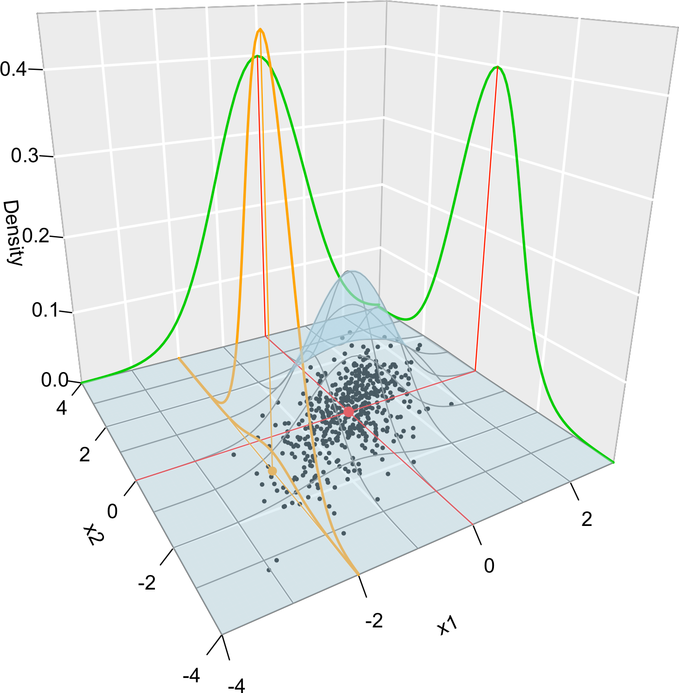
Figure 1.10: Visualization of the joint pdf (in blue), marginal pdfs (green), conditional pdf of \(X_2 \mid X_1=x_1\) (orange), expectation (red point), and conditional expectation \(\mathbb{E}\lbrack X_2 \mid X_1=x_1 \rbrack\) (orange point) of a \(2\)-dimensional normal. The conditioning point of \(X_1\) is \(x_1=-2.\) Note the different scales of the densities, as they have to integrate one over different supports. Note how the conditional density (upper orange curve) is not the joint pdf \(f(x_1,x_2)\) (lower orange curve) with \(x_1=-2\) but a rescaling of this curve by \(\frac{1}{f_{X_1}(x_1)}.\) The parameters of the \(2\)-dimensional normal are \(\mu_1=\mu_2=0,\) \(\sigma_1=\sigma_2=1\) and \(\rho=0.75.\) \(500\) observations sampled from the distribution are shown as black points.

1.4 Transformations of random vectors

The following result allows obtaining the distribution of a random vector \(\boldsymbol{Y}=g(\boldsymbol{X})\) from that of \(\boldsymbol{X},\) if \(g\) is a sufficiently well-behaved function.

Theorem 1.4 (Injective transformation of continuous random vectors) Let \(\boldsymbol{X}\sim f_{\boldsymbol{X}}\) be a continuous random vector in \(\mathbb{R}^p.\) Let \(g=(g_1,\ldots,g_p):\mathbb{R}^p\rightarrow\mathbb{R}^p\) be such that:²⁰

1. \(g\) is injective;²¹
2. the partial derivatives \(\frac{\partial g_i}{\partial x_j} :\mathbb{R}^p\rightarrow\mathbb{R}\) exist and are continuous almost everywhere, for \(i,j=1,\ldots,p;\)
3. for almost all \(\boldsymbol{y}\in\mathbb{R}^p,\) \(\left\|\frac{\partial g^{-1}(\boldsymbol{y})}{\partial \boldsymbol{y}}\right\|\neq0.\)²²

Then, \(\boldsymbol{Y}=g(\boldsymbol{X})\) is a continuous random vector in \(\mathbb{R}^p\) whose pdf is

\[\begin{align*} f_{\boldsymbol{Y}}(\boldsymbol{y})=f_{\boldsymbol{X}}\big(g^{-1}(\boldsymbol{y})\big) \left\|\frac{\partial g^{-1}(\boldsymbol{y})}{\partial \boldsymbol{y}}\right\|,\quad \boldsymbol{y}\in\mathbb{R}^p. \end{align*}\]

Example 1.32 Consider the random vector \((X,Y)^\top\) with pdf

\[\begin{align*} f_{(X,Y)}(x,y)=\begin{cases} 2/9,&0<x<3,\ 0<y<x<3, \\ 0,&\text{otherwise.} \end{cases} \end{align*}\]

What are the distributions of \(X+Y\) and \(X-Y\)?

To answer this question, we define

\[\begin{align*} g(x,y)=(x+y,x-y)^\top=(u,v)^\top \end{align*}\]

and seek to apply Theorem 1.4. Since \(g^{-1}(u,v)=((u+v)/2,(u-v)/2)^\top,\) then

\[\begin{align*} \left\|\frac{\partial g^{-1}(\boldsymbol{y})}{\partial \boldsymbol{y}}\right\|=\left\|\begin{pmatrix} 1/2&1/2\\ 1/2&-1/2\\ \end{pmatrix}\right\|=\left|-\frac{1}{4}-\frac{1}{4}\right|=\frac{1}{2}\neq0. \end{align*}\]

Then, Theorem 1.4 is applicable and \((U,V)^\top=g(X,Y)\) has pdf

\[\begin{align*} f_{(U,V)}(u,v)&=f_{(X,Y)}\big(g^{-1}(u,v)\big)\frac{1}{2}\\ &=\begin{cases} 1/9,&0<(u+v)/2<3,\ 0<(u-v)/2<(u+v)/2<3,\\ 0,&\text{otherwise.} \end{cases} \end{align*}\]

Observe that \(V>0\) by definition. Hence, we can rewrite \(f_{(U,V)}(u,v)=\frac{1}{9}1_{\{(u,v)^\top\in S\}},\) where the support \(S=\{(u,v)^\top\in\mathbb{R}^2:0<v<6-u,\ 0<v<u\}\) is a triangular region delimited by \(v=0,\) \(u=v,\) and \(u+v=6\) (a triangle with vertexes on \((0,0),\) \((3,3),\) and \((6,0)\) — draw it for graphical insight!).

This insight is important to compute the marginals of \((U,V),\) which give the distributions of \(X+Y\) and \(X-Y\):

\[\begin{align*} f_{U}(u)&=\int_{\mathbb{R}} \frac{1}{9}1_{\{(u,v)^\top\in S\}}\,\mathrm{d}v=\begin{cases} \int_{0}^{u}1/9\,\mathrm{d}v=u/9,& u\in(0,3),\\ \int_{0}^{6-u}1/9\,\mathrm{d}v=(6-u)/9,&u\in(3,6),\\ 0,&\text{otherwise,} \end{cases}\\ f_{V}(v)&=\int_{\mathbb{R}} \frac{1}{9}1_{\{(u,v)^\top\in S\}}\,\mathrm{d}u=\begin{cases} \int_{v}^{6-v}1/9\,\mathrm{d}u=(6-2v)/9,& v\in(0,3),\\ 0,&\text{otherwise.} \end{cases} \end{align*}\]

Remark. If the function \(g\) is only injective over the support of \(\boldsymbol{X},\) Theorem 1.4 still can be applied. For example, \(g(x)=\sin(x)\) is (in particular) injective in \((-\pi/2,\pi/2),\) but is not injective in \(\mathbb{R}.\) Following with the example, the pdf of \(Y=\sin(X)\) if \(X\sim \mathcal{U}(0,\pi/2)\) is

\[\begin{align*} f_Y(y)=\frac{2}{\pi} \left|\frac{\mathrm{d}}{\mathrm{d} y}\arcsin(y)\right| 1_{\left\{\arcsin(y)\in \left(0,\tfrac{\pi}{2}\right)\right\}}=\frac{2}{\pi\sqrt{1-y^2}} 1_{\{y\in (0,1)\}}. \end{align*}\]

What if we wanted to know the distribution of the random variable \(Z=g_1(\boldsymbol{X})\) from that of the random vector \(\boldsymbol{X}\sim f_{\boldsymbol{X}}\)? The trick done in the example above points towards the approach to solve this case. Since \(g_1:\mathbb{R}^p\rightarrow\mathbb{R},\) we cannot directly apply Theorem 1.4. However, what we can do is:

1. Complement \(g_1\) to \(g:\mathbb{R}^p\rightarrow\mathbb{R}^p\) so that \(g\) satisfies Theorem 1.4. For example, by defining \(g(\boldsymbol{x})=(g_1(\boldsymbol{x}),x_2,\ldots,x_p)\) (this heavily depends on the form of \(g_1\)).
2. Marginalize \(\boldsymbol{Y}=g(\boldsymbol{X})\) to get the first marginal pdf, i.e., the pdf of \(Z.\)

The next corollary works out the application of the previous principle for sums of independent random variables.

Corollary 1.2 (Sum of independent and continuous random variables) Let \(X_i\sim f_{X_i},\) \(i=1,\ldots,n,\) be independent and continuous random variables. The pdf of \(S:=X_1+\cdots+X_n\) is

\[\begin{align} f_S(s)=\int_{\mathbb{R}^{n-1}} f_{X_1}(s-x_2-\cdots-x_{n}) f_{X_2}(x_2)\cdots f_{X_n}(x_n) \,\mathrm{d} x_2\cdots\,\mathrm{d} x_n. \tag{1.10} \end{align}\]

Proof (Proof of Corollary 1.2). The pdf of \(S\) can be obtained using the transformation

\[\begin{align*} g\begin{pmatrix}x_1\\x_2\\\vdots\\x_n\end{pmatrix}=\begin{pmatrix}x_1+\cdots+x_n\\x_2\\\vdots\\x_n\end{pmatrix},\quad g^{-1}\begin{pmatrix}y_1\\y_2\\\vdots\\y_n\end{pmatrix}=\begin{pmatrix}y_1-y_2-\cdots-y_n\\y_2\\\vdots\\y_n\end{pmatrix} \end{align*}\]

with

\[\begin{align*} \left\|\frac{\partial g^{-1}(\boldsymbol y)}{\partial \boldsymbol y}\right\|=\left\|\begin{pmatrix} 1 & -1 & \cdots & -1\\ 0 & 1 & \cdots & 0 \\ \vdots & \vdots & \ddots & \vdots \\ 0 & 0 & \cdots & 1 \\ \end{pmatrix}\right\|=1 \end{align*}\]

Because of Theorem 1.4 and independence, the pdf of \(\boldsymbol{Y}=g(\boldsymbol{X})\) is

\[\begin{align*} f_{\boldsymbol{Y}}(\boldsymbol{y})&=f_{\boldsymbol{X}}(y_1-y_2-\cdots-y_n,y_2,\ldots,y_n)\\ &=f_{X_1}(y_1-y_2-\cdots-y_n)f_{X_2}(y_2)\cdots f_{X_n}(y_n). \end{align*}\]

A posterior marginalization for \(Y_1=S\) gives

\[\begin{align*} f_{Y_1}(y_1)=\int_{\mathbb{R}^{n-1}} f_{X_1}(y_1-y_2-\cdots-y_n)f_{X_2}(y_2)\cdots f_{X_n}(y_n)\, \mathrm{d}y_2\cdots\, \mathrm{d}y_n. \end{align*}\]

Remark. Care is needed on the domain of integration of (1.10), which is implicitly informed by the domains of \(f_{X_1}\) and \(f_{X_2}.\)

There are more cumbersome or challenging situations involving transformations of random vectors than those covered by Theorem 1.4. For example, those dealing with a transformation \(g\) that is non-injective over the support of \(\boldsymbol{X}.\) In that case, roughly speaking, one needs to break the support of \(\boldsymbol{X}\) into “injective pieces” \(\Delta_1,\Delta_2,\ldots\) for which \(g\) is injective, apply Theorem 1.4 in each of the pieces, and then combine adequately the resulting pdfs.

Theorem 1.5 (Non-injective transformation of continuous random vectors) Let \(\boldsymbol{X}\sim f_{\boldsymbol{X}}\) be a continuous random vector in \(\mathbb{R}^p.\) Let \(g:\mathbb{R}^p\rightarrow\mathbb{R}^p\) be such that:

1. There exists a partition \(\Delta_1,\Delta_2,\ldots\) of \(\mathbb{R}^p\) where the restrictions of \(g\) to each \(\Delta_i,\) denoted by \(g_{\Delta_i},\) are injective.
2. All the functions \(g_{\Delta_i}:\mathbb{R}^p\rightarrow\mathbb{R}^p\) verify the assumptions ii and iii of Theorem 1.4.

Then \(\boldsymbol{Y}=g(\boldsymbol{X})\) is a continuous random vector in \(\mathbb{R}^p\) whose pdf is

\[\begin{align} f_{\boldsymbol{Y}}(\boldsymbol{y})=\sum_{\{i :\ \boldsymbol{y}\in g_{\Delta_i}(\Delta_i)\}} f_{\boldsymbol{X}}\big(g_{\Delta_i}^{-1}(\boldsymbol{y})\big) \left\|\frac{\partial g_{\Delta_i}^{-1}(\boldsymbol{y})}{\partial \boldsymbol{y}}\right\|,\quad \boldsymbol{y}\in\mathbb{R}^p.\tag{1.11} \end{align}\]

Figure 1.11: Non-injective function \(g.\)

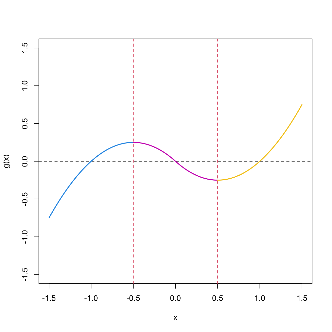
Figure 1.12: Injective partition \(\Delta_i,\) \(i=1,2,3,\) and injective restrictions \(g_{\Delta_i}.\)

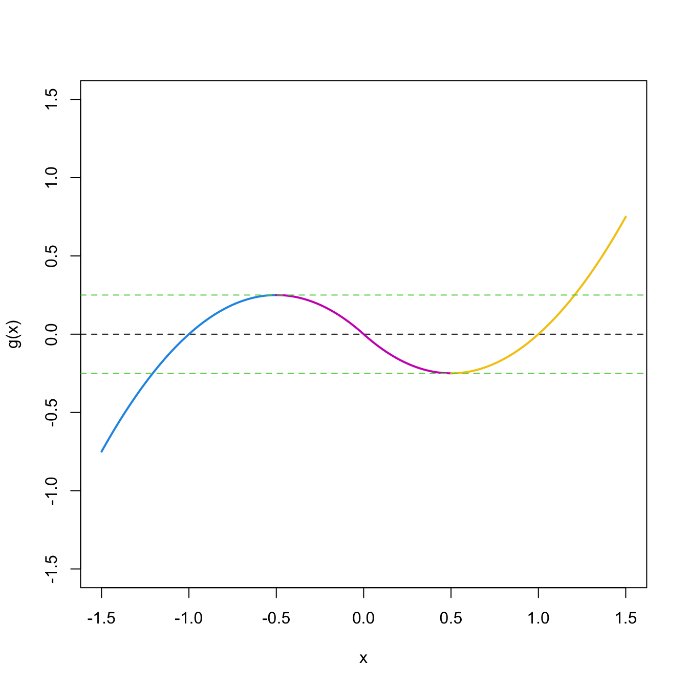
Figure 1.13: Limits of \(g_{\Delta_i}(\Delta_i),\) \(i=1,2,3.\)

Example 1.33 Consider \(g(x)=-x(x+1)1_{\{x<0\}}+x(x-1)1_{\{x>0\}}.\) This is a very smooth function, but is non-injective (e.g., \(-1,\) \(0,\) and \(1\) all map to zero, see Figure 1.11). We can see what are its relative extrema to determine the injective regions: \(\frac{\mathrm{d} g(x)}{\mathrm{d} x}=-(2x+1)_{\{x<0\}}+(2x-1)1_{\{x>0\}}=0\iff x=\pm 1/2.\) This gives the following partition for which \(g\) is piecewise injective (see Figure 1.12):²³

\[\begin{align*} \Delta_1=(-\infty, -1/2],\ \Delta_2=(-1/2, 1/2),\text{ and } \Delta_3=[1/2,\infty). \end{align*}\]

Now, for each \(\Delta_i,\) we can invert \(g_{\Delta_i}.\) For that, we keep in mind where \(g_{\Delta_i}\) are mapping at, i.e., what are \(g_{\Delta_i}(\Delta_i)\) (see Figure 1.13):

1. For \(y\in g_{\Delta_1}(\Delta_1)=(-\infty,1/4],\) \(g_{\Delta_1}^{-1}(y)=(-1-\sqrt{1-4y})/2\) from solving \(y=-x^2-x.\) Then, \(\frac{\mathrm{d} g_{\Delta_1}^{-1}(y)}{\mathrm{d} y}=(1-4y)^{-1/2}.\)

2. For \(y\in g_{\Delta_2}(\Delta_2)=(-1/4,1/4),\) \[\begin{align*} g_{\Delta_2}^{-1}(y)=\begin{cases} (1-\sqrt{1+4y})/2,& y\in(-1/4,0),\\ (-1+\sqrt{1-4y})/2,& y\in(0,1/4) \end{cases} \end{align*}\] from solving \(y=-x^2-x\) and \(y=x^2-x,\) respectively. Then, \[\begin{align*} \frac{\mathrm{d} g_{\Delta_2}^{-1}(y)}{\mathrm{d} y}=\begin{cases} -(1+4y)^{-1/2},& y\in(-1/4,0),\\ -(1-4y)^{-1/2},& y\in(0,1/4). \end{cases} \end{align*}\]

3. For \(y\in g_{\Delta_3}(\Delta_3)=[-1/4,\infty),\) \(g_{\Delta_3}^{-1}(y)=(1+\sqrt{1+4y})/2\) from solving \(y=x^2-x.\) Then, \(\frac{\mathrm{d} g_{\Delta_3}^{-1}(y)}{\mathrm{d} y}=(1+4y)^{-1/2}.\)

   Observe that \(g_{\Delta_i}(\Delta_i),\) \(i=1,2,3\) are overlapping! This is what (1.11) is implicitly warning us with its variable sum: when there is no overlapping, only one pdf is in the sum, but when there is, then several pdfs will enter the sum. We can now proceed applying (1.11) for any \(f_X\):

\[\begin{align*} f_Y(y)=&\;\sum_{\{i :\ y\in g_{\Delta_i}(\Delta_i)\}} f_X\big(g_{\Delta_i}^{-1}(y)\big) \left|\frac{\mathrm{d} g_{\Delta_i}^{-1}(y)}{\mathrm{d} y}\right|\\ =&\;\begin{cases} f_X\big(g_{\Delta_1}^{-1}(y)\big) \left|\frac{\mathrm{d} g_{\Delta_1}^{-1}(y)}{\mathrm{d} y}\right| ,&y\in(-\infty,-1/4],\\ \sum_{i=1}^3 f_X\big(g_{\Delta_i}^{-1}(y)\big) \left|\frac{\mathrm{d} g_{\Delta_i}^{-1}(y)}{\mathrm{d} y}\right| ,&y\in(-1/4,1/4),\\ f_X\big(g_{\Delta_3}^{-1}(y)\big) \left|\frac{\mathrm{d} g_{\Delta_3}^{-1}(y)}{\mathrm{d} y}\right| ,&y\in[1/4,\infty). \end{cases} \end{align*}\]

Remark. The collection \(\Delta_1,\Delta_2,\ldots\) that injectivizes \(g\) might not be finite. For example, if \(g(x)=\sin(x),\) then such collection is \(\{\Delta_k\}_{k\in\mathbb{Z}}\) with \(\Delta_k=(-\pi/2+k\pi,\pi/2+k\pi)\) (Figure 1.14).

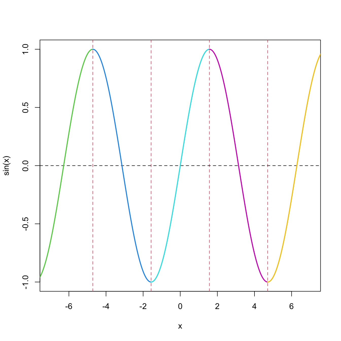
Figure 1.14: Injective regions of the sine function, marked in different colors separated by vertical dashed lines. There is an infinite number of injective regions.

Exercises

Probability review

Exercise 1.1 Let \((\Omega,\mathcal{A},\mathbb{P})\) be a probability space. Prove that, for each \(B\in\mathcal{A}\) with \(\mathbb{P}(B)>0,\) \(\mathbb{P}(\cdot \mid B):\mathcal{A}\rightarrow[0,1]\) is a probability function on \((\Omega,\mathcal{A}),\) and hence \((\Omega,\mathcal{A},\mathbb{P}(\cdot \mid B))\) is a probability space.

Exercise 1.2 Prove that if \(A_1,\ldots,A_k\) are independent events, then

\[\begin{align*} \mathbb{P}\left(\bigcup_{i=1}^kA_i\right)=1-\prod_{i=1}^k(1-\mathbb{P}(A_i)). \end{align*}\]

Exercise 1.3 Prove the law of total probability by expanding \(\mathbb{P}(B)=\mathbb{P}\big(B\cap\big(\cup_{i=1}^k A_i\big)\big)\) (why?).

Exercise 1.4 Prove Bayes’ theorem from the law of total probability and the definition of conditional probability.

Exercise 1.5 Consider the discrete sample space \(\Omega=\{a,b,c,d\}\) and the mapping \(X: \Omega\rightarrow \mathbb{R}\) such that \(X(a)=X(b)=0\) and \(X(c)=X(d)=1.\) Consider the \(\sigma\)-algebra generated by the sets \(\{a\}\) and \(\{c,d\}.\) Prove that \(X\) is a rv for this \(\sigma\)-algebra.

Exercise 1.6 Consider the \(\sigma\)-algebra generated by the subsets \(\{a\}\) and \(\{c\}\) for \(\Omega=\{a,b,c,d\}.\)

1. Prove that the mapping in Exercise 1.5 is not a rv for this \(\sigma\)-algebra.
2. Define a mapping that is a rv for this \(\sigma\)-algebra.

Exercise 1.7 Consider the experiment consisting in tossing two times a coin.

1. Provide the sample space.
2. For the \(\sigma\)-algebra \(\mathbb{P}(\Omega),\) consider the rv \(X=\) “Number of heads in two tosses”. Provide the range and the probability function induced by \(X.\)

Exercise 1.8 For the experiment of Exercise 1.7, consider the rv \(Y=\) “Difference between the number of heads and the number of tails”. Obtain its range and its induced probability function.

Exercise 1.9 A dice is rolled two times. Obtain the sample space and the pmf of the following rv’s:

1. \(X_1=\) “Sum of the resulting numbers”.
2. \(X_2=\) “Absolute value of difference of the resulting numbers”.
3. \(X_3=\) “Maximum of the resulting numbers”.
4. \(X_4=\) “Minimum of the resulting numbers”.

Indicate, for each case, which is the pre-image by the corresponding rv of the set \([1.5,3.5]\) and which is its induced probability.

Random variables

Exercise 1.10 Assume that the lifespan (in hours) of a fluorescent tube is represented by the continuous rv \(X\) with pdf

\[\begin{align*} f(x)=\begin{cases} c/x^2, & x>100,\\ 0, & x\leq 100. \end{cases} \end{align*}\]

Compute:

1. The value of \(c.\)
2. The cdf of \(X.\)
3. The probability that a tube lasts more than \(500\) hours.

Exercise 1.11 When storing flour in bags of \(100\) kg, a random error \(X\) is made in the measurement of the weight of the bags. The pdf of the error \(X\) is given by

\[\begin{align*} f(x)=\begin{cases} k(1-x^2), & -1<x<1,\\ 0, & \text{otherwise}. \end{cases} \end{align*}\]

1. Compute the probability that a bag weighs more than \(99.5\) kg.
2. What is the percentage of bags with a weight between \(99.8\) and \(100.2\) kg?

Exercise 1.12 A rv only takes the values \(1\) and \(3\) with a non-zero probability. If its expectation is \(8/3,\) find the probabilities of these two values.

Exercise 1.13 The random number of received calls in a call center during a time interval of \(h\) minutes, \(X_h,\) has a pmf

\[\begin{align*} \mathbb{P}(X_h=n)=\frac{(5h)^n}{n!}e^{-5h}, \quad n=0,1,2,\ldots. \end{align*}\]

1. Find the average number of calls received in half an hour.
2. What is the expected time that has to pass until an average of \(100\) calls is received?

Exercise 1.14 Let \(X\) be a rv following a Poisson distribution (see Example 1.14). Compute the expectation and variance of the new rv

\[\begin{align*} Y=\begin{cases} 1 & \mathrm{if}\ X=0,\\ 0 & \mathrm{if}\ X\neq 0. \end{cases} \end{align*}\]

Exercise 1.15 Consider a rv with density function

\[\begin{align*} f(x)=\begin{cases} 6x(1-x), & 0<x<1,\\ 0, & \mathrm{otherwise}. \end{cases} \end{align*}\]

Compute:

1. \(\mathbb{E}[X]\) and \(\mathbb{V}\mathrm{ar}[X].\)
2. \(\mathbb{P}\left(|X-\mathbb{E}[X]|<\sqrt{\mathbb{V}\mathrm{ar}[X]}\right).\)

Moment generating function

Exercise 1.16 For each of the pmf’s given below, find the mgf and, using it, obtain the expectation and variance of the corresponding rv.

1. \(\mathbb{P}(X=1)=p,\) \(\mathbb{P}(X=0)=1-p,\) where \(p\in(0,1).\)
2. \(\mathbb{P}(X=n)=(1-p)^n p,\) \(n=0,1,2,\ldots,\) where \(p\in(0,1).\)

Exercise 1.17 Compute the mgf of \(\mathcal{U}(0,1).\) Then, use the result to obtain:

1. The mgf of \(\mathcal{U}(-1,1).\)
2. The mgf of \(\sum_{i=1}^n X_i,\) where \(X_i\sim\mathcal{U}(-1/i,1/i).\)
3. \(\mathbb{E}[\mathcal{U}(-1,1)^k],\) \(k\geq 1.\) (You can verify the approach using mgf with direct computation of \(\mathbb{E}[\mathcal{U}(-1,1)^k].\))

Exercise 1.18 Compute the mgf of the following rv’s:

1. \(\mathcal{N}(\mu,\sigma^2).\)
2. \(\mathrm{Exp}(\lambda).\)
3. \(X\sim f(\cdot;\theta)\) given in (1.13).

Exercise 1.19 Compute the mgf of \(X\sim \mathrm{Pois}(\lambda).\)

Exercise 1.20 (Poisson additive property) Prove the additive property of the Poisson distribution, that is, prove that if \(X_i,\) \(i=1,\ldots,n\) are independent rv’s with respective distributions \(\mathrm{Pois}(\lambda_i),\) \(i=1,\ldots,n,\) then

\[\begin{align*} \sum_{i=1}^n X_i\sim \mathrm{Pois}\left(\sum_{i=1}^n\lambda_i\right). \end{align*}\]

Exercise 1.21 (Gamma additive property) Prove the additive property of the gamma distribution, that is, prove that if \(X_i,\) \(i=1,\ldots,n\) are independent rv’s with respective distributions \(\Gamma(\alpha_i,\beta),\) \(i=1,\ldots,n,\) then

\[\begin{align*} \sum_{i=1}^n X_i\sim \Gamma\left(\sum_{i=1}^n\alpha_i,\beta\right). \end{align*}\]

Random vectors

Exercise 1.22 Conclude Example 1.27 by computing the cdf function for all \((x_1,x_2)^\top\in\mathbb{R}^2.\) Split \(\mathbb{R}^2\) into key regions for doing that.

Exercise 1.23 Consider the random vector \((X,Y)^\top\) with joint pdf

\[\begin{align*} f(x,y)=e^{-x}, \quad x>0,\ 0<y<x. \end{align*}\]

Compute \(\mathbb{E}[X],\) \(\mathbb{E}[Y],\) and \(\mathrm{Cov}[X,Y].\)

Exercise 1.24 Obtain the marginal pdf and cdf of \(X_2\) in Example 1.26.

Exercise 1.25 Obtain the marginal cdf and pmf of \(X_1\) in Example 1.27.

Exercise 1.26 Consider the joint pdf of the random vector \((X,Y)^\top\):

\[\begin{align*} f(x,y)=\begin{cases} cx^{-2}y^{-3},&x>50,\ y>10,\\ 0,&\text{otherwise.} \end{cases} \end{align*}\]

1. Find \(c\) such that \(f\) is a pdf.
2. Find the marginal pdf of \(X.\)
3. Find the marginal cdf of \(X.\)
4. Compute \(\mathbb{P}(X>100,Y>10).\)

Exercise 1.27 Consider the joint pdf of the random vector \((X,Y)^\top\):

\[\begin{align*} f(x,y)=\begin{cases} K(x^2+y^2),&2\leq x\leq 3,\ 2\leq y\leq 3,\\ 0,&\text{otherwise.} \end{cases} \end{align*}\]

1. Find the value of \(K\) such that \(f\) is a pdf.
2. Find the marginal pdf of \(X.\)
3. Compute \(\mathbb{P}(Y>2.5).\)

Exercise 1.28 Obtain the pdfs of \(Y \mid X=x\) and \(X \mid Y=y\) in Exercise 1.26 applying (1.4). Check that the conditional pdf integrates one for each possible value \(y.\)

Exercise 1.29 Repeat Exercise 1.28 but using the pdf given on Exercise 1.27.

Exercise 1.30 Compute the conditional cdfs of \(Y \mid X=x\) and \(X \mid Y=y\) in Exercise 1.26. Do they equal \(y\mapsto F(x,y)/F_X(x)\) and \(x\mapsto F(x,y)/F_Y(y)\)?²⁴

Exercise 1.31 Compute variance-covariance matrix of the random vector with pdf given in Exercise 1.27.

Exercise 1.32 Prove that \(\mathbb{E}[\mathrm{Exp}(\lambda)]=1/\lambda\) and \(\mathbb{V}\mathrm{ar}[\mathrm{Exp}(\lambda)]=1/\lambda^2.\)

Transformations of random vectors

Exercise 1.33 Let \(\boldsymbol{X}\sim f_{\boldsymbol{X}}\) in \(\mathbb{R}^p.\) Show that:

1. For \(a\neq0,\) \(a\boldsymbol{X}\sim f_{\boldsymbol{X}}(\cdot/a)/|a|^p.\)
2. For a \(p\times p\) rotation matrix²⁵ \(\boldsymbol{R},\) \(\boldsymbol{R}\boldsymbol{X}\sim f_{\boldsymbol{X}}\left(\boldsymbol{R}^\top \cdot \right).\)

Exercise 1.34 Consider the random vector \((X,Y)^\top\) with pdf

\[\begin{align} f(x,y)=\begin{cases} K(1 - x^2-y^2),& (x,y)^\top\in S, \\ 0,&\text{otherwise.} \end{cases} \tag{1.12} \end{align}\]

Obtain:

1. The support \(S\) and \(K>0.\)
2. The pdf of \(X+Y.\)
3. The pdf of \(XY.\)

Exercise 1.35 Let \(X_1,\ldots,X_n\sim\Gamma(1,\theta)\) independent. Using only Corollary 1.2, compute the pdf of:

1. \(X_1+X_2.\)
2. \(X_1+X_2+X_3.\)
3. \(X_1+\cdots+X_n.\)

Exercise 1.36 Corroborate the usefulness of Proposition 1.10 by computing the following expectations as (1) \(\mathbb{E}[g(X)]=\int g(x)f_X(x)\,\mathrm{d}x\) and (2) \(\mathbb{E}[Y]=\int yf_Y(y)\,\mathrm{d}y,\) where \(Y=g(X).\)

1. \(X\sim \mathcal{U}(0,1)\) and \(g(x)=x^2.\)
2. \(X\sim \mathrm{Exp}(1)\) and \(g(x)=e^x.\)

Exercise 1.37 Consider \(X\sim \mathcal{U}(-2,2)\) and \(Y=g(X),\) with \(g\) as in Example 1.33. Plot the density function \(f_Y\) and explain the intuition of why it has such a “Sauron-inspired” shape. You can validate the form of \(f_Y\) by simulating random values for \(Y\) and drawing its histogram.

Exercise 1.38 Let \(X\sim \mathcal{N}(0,1).\) Compute the pdf of \(X^2.\)

Exercise 1.39 Let \((X,Y)^\top\sim \mathcal{N}_2(\boldsymbol{0},\boldsymbol{I}_2).\) Compute the pdf of \(X^2+Y^2.\) Then, compute the pdf of \(-2\log U,\) where \(U\sim\mathcal{U}(0,1).\) Is there any connection between both pdfs?

Exercise 1.40 Validate the densities of \(X+Y\) and \(XY\) from Exercise 1.33 with a simulation. To do so:

1. Compute the pdf of \(R=\sqrt{1-\sqrt{U}}\) with \(U\sim\mathcal{U}(0,1).\)
2. Show that \((X,Y)^\top=(R\cos\Theta,R\sin\Theta)^\top,\) with \(\Theta\sim\mathcal{U}(0,2\pi)\) independent from \(R,\) actually follows the pdf (1.12).
3. Simulate \(X+Y\) and draw its histogram. Overlay \(f_{X+Y}.\)
4. Simulate \(XY\) and draw its histogram. Overlay \(f_{XY}.\)

Exercise 1.41 Consider the random variable \(X\) with pdf

\[\begin{align} f(x;\theta)=\frac{\theta}{\pi(\theta^2+x^2)},\quad x\in\mathbb{R},\ \theta>0.\tag{1.13} \end{align}\]

Obtain the pdf of \(Y=X\mod 2\pi.\)

---

1. Note this definition frees the mathematical meaning of probability from the “tyranny” of the random experiment by abstracting the concept of probability.↩︎

2. “Theorem” might be an overstatement for this result, which is obtained from two lines of mathematics. That is why it is many times known as the Bayes formula.↩︎

3. The following is an analogy with the hierarchy in computer languages: \((\mathbb{R},\mathcal{B})\) is the high-level programming language, \(X\) is the compiler, and \((\Omega,\mathcal{A})\) is the low-level programming language that is run by the machine.↩︎

4. That is, \(\lim_{x\to a+} F_X(x)=F(a),\) for all \(a\in\mathbb{R}.\)↩︎

5. This terminology stems from the fact that the existence of \(f_X\) such that condition (1.2) holds is equivalent to \(F_X\) being an absolutely continuous function. As the famous counterexample given by the Cantor function, absolute continuity is a more strict requirement than continuity.↩︎

6. “Almost all” meaning that a finite or countable number of points is excluded.↩︎

7. Observe \(\int_{(a,b)} f_X(t)\,\mathrm{d}t=\int_a^b f_X(t)\,\mathrm{d}t.\)↩︎

8. “\(\mathrm{d}F_X(x)\)” is just a fancy way of combining the continuous case (integral) and discrete case (sum) within the same notation. The precise mathematical meaning of “\(\mathrm{d}F_X(x)\)” is the Riemann–Stieltjes integral.↩︎

9. See the forthcoming “Law of the unconscious statistician” in Proposition 1.10.↩︎

10. The possible non-existence can be removed considering the characteristic function \(\varphi_X(t)=\mathbb{E}\left[e^{\mathrm{i}tX}\right],\) which exists for all \(t\in\mathbb{R}.\) However, it comes at the expense of having a complex-valued function (\(\mathrm{i}=\sqrt{-1}\) is the imaginary unit). The properties of the mgf and characteristic function are almost equivalent since \(\varphi_X(-\mathrm{i}t)=M_X(t).\)↩︎

11. Observe if \(r\) in (1.3) is a natural number, then the standard binomial theorem arises since \(\binom{r}{x}=0\) when \(x>r\): \((a+b)^r =\sum_{x=0}^{r} \binom{r}{x} a^x b^{r-x}.\)↩︎

12. A formal definition of independence of rv’s is given in the forthcoming Definition 1.34.↩︎

13. This concept will be precised in the forthcoming Definition 2.6.↩︎

14. Why the transpose symbol \(^\top\) in \((X_1(\omega),\ldots,X_p(\omega))^\top\)? This is to indicate that \((X_1(\omega),\ldots,X_p(\omega)),\) a row matrix, has to be transposed, so that it becomes the column matrix \(\begin{pmatrix}X_1(\omega)\\\vdots\\X_p(\omega)\end{pmatrix}.\) Vectors are almost always understood in mathematics as column matrices, which is inconvenient for displaying. It is easy to run into inconsistent matrix multiplications if one does not honor the column layout of vectors via the transpose operator.↩︎

15. That is, \(\lim_{\boldsymbol{x}\to\boldsymbol{a}+} F_{\boldsymbol{X}}(\boldsymbol{a})=F(\boldsymbol{a}),\) for all \(\boldsymbol{a}\in\mathbb{R}^p.\)↩︎

16. “Almost all” meaning that we exclude a finite or countable number of points and “zero-measure” sets. Zero-measure sets are those with a lower dimension than \(p\) (e.g., a curve in \(\mathbb{R}^2\)).↩︎

17. Observe \(\int_{(a_1,b_1)\times\stackrel{p}{\cdots}\times(a_p,b_p)} f_{\boldsymbol{X}}(\boldsymbol{t})\,\mathrm{d}\boldsymbol{t}=\int_{a_1}^{b_1}\stackrel{p}{\cdots}\int_{a_p}^{b_p} f_{\boldsymbol{X}}(\boldsymbol{t})\,\mathrm{d}t_p\cdots\,\mathrm{d}t_1.\)↩︎

18. Or random vector.↩︎

19. Observe that the two parameters of this probability model are precisely its expectation vector and variance-covariance matrix. Not all the probability models have parameters relating so neatly with these two concepts!↩︎

20. The functions \(g_i:\mathbb{R}^p\rightarrow\mathbb{R}\) are the components of \(g=(g_1,\ldots,g_p).\)↩︎

21. Therefore, \(g\) has an inverse \(g^{-1}.\)↩︎

22. The term \(\left\|\frac{\partial g^{-1}(\boldsymbol{y})}{\partial \boldsymbol{y}}\right\|\) is the absolute value of the determinant of the \(p\times p\) Jacobian matrix \(\frac{\partial g^{-1}(\boldsymbol{y})}{\partial \boldsymbol{y}}=\left(\frac{\partial g_i^{-1}(\boldsymbol{y})}{\partial y_j}\right)_{ij}.\)↩︎

23. It would not matter if we were leaving out of the partition a finite number of points.↩︎

24. The notation \(x\mapsto x^2\) is a quick way of defining an unnamed function that maps \(x\) onto \(x^2.\)↩︎

25. That is, such that \(\boldsymbol{R}^{-1}=\boldsymbol{R}^\top\) and \(|\boldsymbol{R}|=\pm1.\)↩︎