2 Introduction

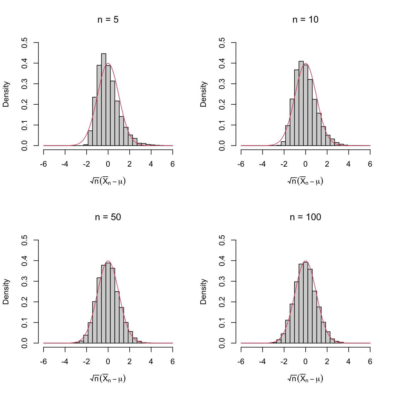
Figure 2.1: Histograms of \(\sqrt{n}(\bar{X}_n-\mu)\) for independent rv’s \(X_1,\ldots,X_n\) with expectation \(\mu\) and variance \(\sigma^2.\) The pdf of \(\mathcal{N}(0,\sigma^2)\) is superimposed in red. A clear convergence appears, despite \(X_1,\ldots,X_n\sim\mathrm{Exp}(1)\) being heavily non-normal. The culprit is the Central Limit Theorem.

This chapter introduces the basic elements in statistical inference and proves the simplest case of the central limit theorem.

2.1 Basic definitions

As seen in Example 1.3, employing frequentist ideas we can state that there is an underlying probability law that drives any random experiment. The interest of statistical inference when studying a random phenomenon lies on learning this underlying distribution.

Usually, for certain kinds of experiments and random variables, experience provides some information about the underlying distribution \(F\) (identified here with the cdf). In many situations, \(F\) is not exactly known, but we may know the approximate form of \(F\) up to a parameter \(\theta\) that drives its shape. In other words, we may know that \(F\) belongs to a parametric family of distributions \(\{F(\cdot;\theta): \theta\in\Theta\}\) that is indexed by a certain parameter \(\theta\in\Theta.\) For example, the class of distributions \(\{\Phi(\cdot/\sigma):\sigma\in\mathbb{R}_+\}\) (remember Example 1.17) contains all the normal distributions \(\mathcal{N}(0,\sigma^2)\) and is indexed by the standard deviation parameter \(\sigma.\)

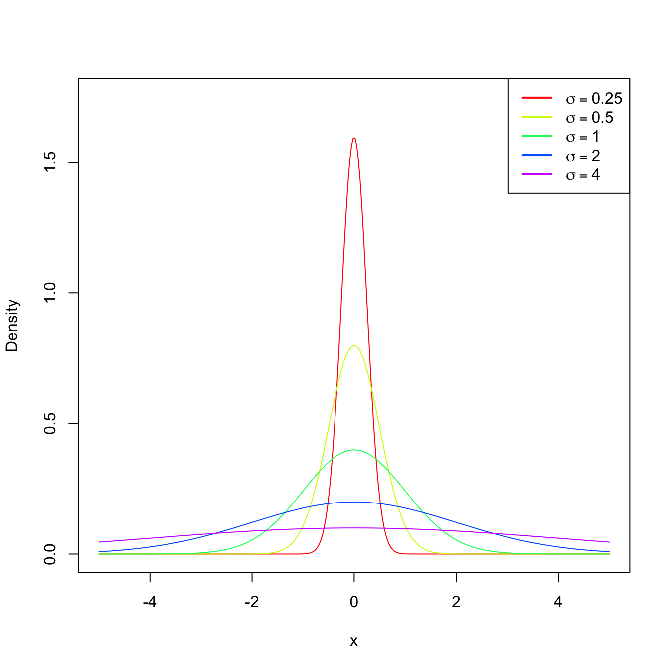
Figure 2.2: \(\mathcal{N}(0,\sigma^2)\) pdf’s for several standard deviations \(\sigma.\)

If our objective is to know more about \(F\) or, equivalently, about its driving parameter \(\theta,\) we can perform independent realizations of the experiment and then process the information in a certain way to infer knowledge about \(F\) or \(\theta.\) This is the process of performing statistical inference about \(F\) or, equivalently, about \(\theta.\) The fact that we perform independent repetitions of the experiment means that, for each repetition of the experiment, we have an associated rv with the same distribution \(F.\) This is the concept of a simple random sample.

Definition 2.1 (Simple random sample and sample realization) A simple random sample (srs) of size \(n\) of a rv \(X\) with distribution \(F\) is a collection of rv’s \((X_1,\ldots,X_n)\) that are independent and identically distributed (iid) with the distribution \(F.\) A sample realization is the set of observed values \((x_1,\ldots,x_n)\) of \((X_1,\ldots,X_n).\)

Therefore, a srs is a random vector \(\boldsymbol{X}=(X_1,X_2,\ldots,X_n)^\top\) that is defined over the measurable product space \((\mathbb{R}^n,\mathcal{B}^n).\) Since the rv’s are independent, the cdf of the sample (or of the random vector \(\boldsymbol{X}\)) is

\[\begin{align*} F_{\boldsymbol{X}}(x_1,x_2,\ldots,x_n)=F(x_1)F(x_2)\cdots F(x_n). \end{align*}\]

Example 2.1 We analyze next the underlying probability functions that appear in Example 1.3.

1. Consider the family of pmf’s given by \[\begin{align*} \mathbb{P}(X=1)=\theta, \quad \mathbb{P}(X=0)=1-\theta,\quad \theta\in [0,1]. \end{align*}\] The pmf of the first experiment in Example 1.3 belongs to this family, for \(\theta=0.5.\)

2. From previous experience, it is known that the rv that measures the number of events happening in a given time interval has a pmf that belongs to \(\{p(\cdot;\lambda):\lambda\in\mathbb{R}_+\},\) where

   \[\begin{align} p(x;\lambda)=\frac{\lambda^x e^{-\lambda}}{x!}, \quad x=0,1,2,3,\ldots\tag{2.1} \end{align}\] This is the pmf of the Poisson of intensity parameter \(\lambda\) that was introduced in Exercise 1.14. Replacing \(\lambda=4\) and \(x=0,1,2,3,\ldots\) in (2.1), we obtain the following probabilities:

   \(x\)	\(0\)	\(1\)	\(2\)	\(3\)	\(4\)	\(5\)	\(6\)	\(7\)	\(8\)	\(\geq 9\)
   \(p(x;4)\)	\(0.018\)	\(0.073\)	\(0.147\)	\(0.195\)	\(0.156\)	\(0.156\)	\(0.104\)	\(0.060\)	\(0.030\)	\(0.021\)

   Observe that these probabilities are similar to the relative frequencies given in Table 1.2.

3. From previous experience, it is known that the rv that measures the weight of a person follows a normal distribution \(\mathcal{N}(\mu,\sigma^2),\) whose pdf is \[\begin{align*} \phi(x;\mu,\sigma^2)=\frac{1}{\sqrt{2\pi\sigma^2}}\exp\left\{-\frac{(x-\mu)^2}{2\sigma^2}\right\},\quad \mu\in\mathbb{R}, \ \sigma^2\in\mathbb{R}_+. \end{align*}\] Indeed, setting \(\mu=39\) and \(\sigma=5,\) the next probabilities for the intervals are obtained:

   \(I\)	\((-\infty,35]\)	\((35,45]\)	\((45,55]\)	\((55,65]\)	\((65,\infty)\)
   \(\mathbb{P}(X\in I)\)	\(0.003\)	\(0.209\)	\(0.673\)	\(0.114\)	\(0.001\)

   Observe the similarity with Table 1.3.

Given a srs \(X_1,\ldots,X_n,\) inference is carried out by means of “summaries” of this sample. The general definition of such summary is called statistic, and is another key pillar in statistical inference.

Definition 2.2 (Statistic) A statistic \(T\) is any measurable function \(T:(\mathbb{R}^n,\mathcal{B}^n)\rightarrow(\mathbb{R}^k,\mathcal{B}^k),\) where \(k\) is the dimension of the statistic.

A wide variety of statistics is possible given a srs. Definitely not all of them will be as useful for inferential purposes! In particular, the sample itself is always a statistic, but surely not the most interesting one as it does not summarize information about a parameter \(\theta.\)

Example 2.2 The following are examples of statistics:

• \(T_1(X_1,\ldots,X_n)=\frac{1}{n}\sum_{i=1}^n X_i.\)
• \(T_2(X_1,\ldots,X_n)=\frac{1}{n}\sum_{i=1}^n (X_i-\bar{X})^2.\)
• \(T_3(X_1,\ldots,X_n)=\min\{X_1,\ldots,X_n\}=: X_{(1)}.\)
• \(T_4(X_1,\ldots,X_n)=\max\{X_1,\ldots,X_n\}=: X_{(n)}.\)
• \(T_5(X_1,\ldots,X_n)=\sum_{i=1}^n \log X_i.\)
• \(T_6(X_1,\ldots,X_n)=(X_{(1)},X_{(n)})^\top.\)
• \(T_7(X_1,\ldots,X_n)=(X_1,\ldots,X_n)^\top.\)

All the statistics have dimension \(k=1,\) except \(T_6\) with \(k=2\) and \(T_7\) with \(k=n.\)

From the definition, we can see that a statistic is a rv, or a random vector if \(k>1.\) This new rv is a transformation (see Section 1.4) of the random vector \((X_1,\ldots,X_n)^\top.\) The distribution of the statistic \(T\) is called the sampling distribution of \(T\), since it depends on the distribution of the sample and the transformation considered.

We see next some examples on the determination of the sampling distribution of statistics for discrete and continuous rv’s.

Example 2.3 A coin is tossed independently three times. Let \(X_i,\) \(i=1,2,3,\) be the rv that measures the outcome of the \(i\)-th toss:

\[\begin{align*} X_i=\begin{cases} 1 & \text{if H is the outcome of the $i$-th toss},\\ 0 & \text{if T is the outcome of the $i$-th toss}. \end{cases} \end{align*}\]

If we do not know whether the coin is fair (Heads and Tails may not be equally likely), then the pmf of \(X_i\) is given by

\[\begin{align*} \mathbb{P}(X_i=1)=\theta,\quad \mathbb{P}(X_i=0)=1-\theta, \quad \theta\in\Theta=[0,1]. \end{align*}\]

The three rv’s are independent. Therefore, the probability of the sample \((X_1,X_2,X_3)\) is the product of the individual probabilities of \(X_i,\) that is,

\[\begin{align*} \mathbb{P}(X_1=x_1,X_2=x_2,X_3=x_3)=\mathbb{P}(X_1=x_1)\mathbb{P}(X_2=x_2)\mathbb{P}(X_3=x_3). \end{align*}\]

The following table collects the values of the pmf of the sample for each possible value of the sample.

\((x_1,x_2,x_3)\)	\(p(x_1,x_2,x_3)\)
\((1,1,1)\)	\(\theta^3\)
\((1,1,0)\)	\(\theta^2(1-\theta)\)
\((1,0,1)\)	\(\theta^2(1-\theta)\)
\((0,1,1)\)	\(\theta^2(1-\theta)\)
\((1,0,0)\)	\(\theta(1-\theta)^2\)
\((0,1,0)\)	\(\theta(1-\theta)^2\)
\((0,0,1)\)	\(\theta(1-\theta)^2\)
\((0,0,0)\)	\((1-\theta)^3\)

We can define the sum statistic as \(T_1(X_1,X_2,X_3)=\sum_{i=1}^3 X_i.\) Now, from the previous table, we can compute the sampling distribution of \(T\) as the pmf given by

\(t_1=T_1(x_1,x_2,x_3)\)	\(p(t_1)\)
\(3\)	\(\theta^3\)
\(2\)	\(3\theta^2(1-\theta)\)
\(1\)	\(3\theta(1-\theta)^2\)
\(0\)	\((1-\theta)^3\)

To compute the table, we have summed the probabilities \(p(x_1,x_2,x_3)\) of the cases \((x_1,x_2,x_3)\) leading to each value of \(t_1.\)

Another possible statistic is the sample mean, \(T_2(X_1,X_2,X_3)=\bar{X},\) whose sampling distribution is

\(t_2=T_2(x_1,x_2,x_3)\)	\(p(t_2)\)
\(1\)	\(\theta^3\)
\(2/3\)	\(3\theta^2(1-\theta)\)
\(1/3\)	\(3\theta(1-\theta)^2\)
\(0\)	\((1-\theta)^3\)

Example 2.4 Let \((X_1,\ldots,X_n)\) be a srs of a rv with \(\mathrm{Exp}(\theta)\) distribution, that is, with pdf

\[\begin{align*} f(x;\theta)= \theta e^{-\theta x}, \quad x>0, \ \theta>0. \end{align*}\]

We will obtain the sampling distribution of the sum statistic \(T(X_1,\ldots,X_n)=\sum_{i=1}^n X_i.\)

First, observe that \(\mathrm{Exp}(\theta)\stackrel{d}{=}\Gamma(1,1/\theta)\) since the pdf of a \(\Gamma(\alpha,\beta)\) is given by

\[\begin{align} f(x;\alpha,\beta)=\frac{1}{\Gamma(\alpha) \beta^{\alpha}}\, x^{\alpha-1} e^{-x/\beta}, \quad x>0, \ \alpha>0, \ \beta>0. \tag{2.2} \end{align}\]

From Exercise 1.21 we know that the sum of \(n\) independent rv’s \(\Gamma(\alpha,\beta)\) is a \(\Gamma(n\alpha,\beta)\) without the need of using transformations. Therefore, thanks to this shortcut, the distribution of the sum statistic \(T(X_1,\ldots,X_n)=\sum_{i=1}^n X_i\) is a \(\Gamma(n,1/\theta).\)

Example 2.5 Let \((X_1,X_2)\) be a srs of a rv with uniform distribution \(\mathcal{U}(\theta-1,\theta+1),\) \(\theta>0.\) The pdf of this distribution is

\[\begin{align*} f(x;\theta)=\frac{1}{2} 1_{\{x\in(\theta-1,\theta+1)\}}. \end{align*}\]

We obtain the sampling distribution of the average statistic \(T(X_1,X_2)=(X_1+X_2)/2.\) To do so, we use Corollary 1.2 to have first the distribution of \(S=X_1+X_2\):

\[\begin{align*} f_S(s;\theta)&=\int_{\mathbb{R}} f(s-x;\theta)f(x;\theta)\,\mathrm{d} x\\ &=\frac{1}{4}\int_{\mathbb{R}} 1_{\{(s-x)\in(\theta-1,\theta+1)\}}1_{\{x\in(\theta-1,\theta+1)\}}\,\mathrm{d} x\\ &=\frac{1}{4}\int_{\mathbb{R}} 1_{\{x\in(s-\theta-1,s-\theta+1)\}}1_{\{x\in(\theta-1,\theta+1)\}}\,\mathrm{d} x\\ &=\frac{1}{4}\int_{\mathbb{R}} 1_{\{x\in(\max(s-\theta-1,\theta-1),\min(s-\theta+1,\theta+1)\}}\,\mathrm{d} x\\ &=\frac{\min(s-\theta+1,\theta+1)-\max(s-\theta-1,\theta-1)}{4} \end{align*}\]

with \(s\in(2(\theta-1),2(\theta+1)).\) Using Exercise 1.33, the pdf of \(T=S/2\) is therefore

\[\begin{align} f_T(t;\theta)=\frac{\min(2t-\theta+1,\theta+1)-\max(2t-\theta-1,\theta-1)}{2} \tag{2.3} \end{align}\]

with \(t\in(\theta-1,\theta+1).\)

Figure 2.3: Pdf (2.3) for several values of \(\theta.\)

Example 2.6 (Sampling distribution of the minimum) Let \((X_1,\ldots,X_n)\) be a srs of a rv with cdf \(F\) (either discrete or continuous). The sampling distribution of the statistic \(T(X_1,\ldots,X_n)=X_{(1)}\) follows from the cdf of \(T\) using the iid-ness of the sample and the properties of the minimum:

\[\begin{align*} 1-F_T(t) &=\mathbb{P}_T(T>t)=\mathbb{P}_{(X_1,\ldots,X_n)}(X_{(1)}> t)\\ &=\mathbb{P}_{(X_1,\ldots,X_n)}(X_1> t,\ldots,X_n> t)=\prod_{i=1}^n \mathbb{P}_{X_i}(X_i> t)\\ &=\prod_{i=1}^n\left[1-F_{X_i}(t)\right]=\left[1-F(t)\right]^n. \end{align*}\]

2.2 Sampling distributions in normal populations

Many rv’s arising in biology, sociology, or economy can be successfully modeled by a normal distribution with mean \(\mu\in\mathbb{R}\) and variance \(\sigma^2\in \mathbb{R}_+.\) This is due to the central limit theorem, a key result in statistical inference that shows that the accumulated effect of a large number of independent rv’s behaves approximately as a normal distribution. Because of this, and the tractability of normal variables, in statistical inference it is usually assumed that the distribution of a rv belongs to the normal family of distributions \(\{\mathcal{N}(\mu,\sigma^2):\mu\in\mathbb{R},\ \sigma^2\in\mathbb{R}_+\},\) where the mean \(\mu\) and the variance \(\sigma^2\) are unknown.

In order to perform inference about \((\mu,\sigma^2),\) a srs \((X_1,\ldots,X_n)\) from \(\mathcal{N}(\mu,\sigma^2)\) is considered. We can compute several statistics using this sample, but we pay special attention to the ones whose values tend to be “similar” to the value of the unknown parameters \((\mu,\sigma^2).\) A statistic of this kind is precisely an estimator. Different kinds of estimators exist depending on the criterion employed to define the “similarity” between the estimator and the parameter to be estimated.

The sample mean \(\bar{X}\) and sample variance \(S^2\) estimators play an important role in statistical inference, since both are “good” estimators of \(\mu\) and \(\sigma^2,\) respectively. As a consequence, it is important to obtain their sampling distributions in order to know their random behaviors. We will do so under the assumption of normal populations.

2.2.1 Sampling distribution of the sample mean

Theorem 2.1 (Distribution of \(\bar{X}\)) Let \((X_1,\ldots,X_n)\) be a srs of size \(n\) of a rv \(\mathcal{N}(\mu,\sigma^2).\) Then, the sample mean \(\bar{X}:=\frac{1}{n}\sum_{i=1}^n X_i\) satisfies \[\begin{align} \bar{X}\sim\mathcal{N}\left(\mu,\frac{\sigma^2}{n}\right). \tag{2.4} \end{align}\]

Proof (Proof of Theorem 2.1). The proof is simple and can actually be done using the mgf through Exercise 2.1 and Proposition 1.5.

Alternatively, assuming that the sum of normal rv’s is another normal (Exercise 2.1), it only remains to compute the resulting mean and variance. The mean is directly obtained from the properties of the expectation, requiring neither the assumption of normality nor independence:

\[\begin{align*} \mathbb{E}[\bar{X}]=\frac{1}{n}\sum_{i=1}^n \mathbb{E}[X_i] =\frac{1}{n}n\mu=\mu. \end{align*}\]

The variance is obtained by relying only on the hypothesis of independence:

\[\begin{align*} \mathbb{V}\mathrm{ar}[\bar{X}]=\frac{1}{n^2}\sum_{i=1}^n \mathbb{V}\mathrm{ar}[X_i]=\frac{1}{n^2}n\sigma^2=\frac{\sigma^2}{n}. \end{align*}\]

Let us see some practical applications of this result.

Example 2.7 It is known that the weight (in grams) of liquid that a machine fills into a bottle follows a normal distribution with unknown mean \(\mu\) and standard deviation \(\sigma=25\) grams. From the production of the filling machine along one day, it is obtained a srs of \(n=9\) filled bottles. We want to know what is the probability that the sample mean is closer than \(8\) grams to the real mean \(\mu.\)

If \(X_1,\ldots,X_9\) is the srs that contains the measurements of the nine bottles, then \(X_i\sim\mathcal{N}(\mu,\sigma^2),\) \(i=1,\ldots,n,\) where \(n=9\) and \(\sigma^2=25^2.\) Then, by Theorem 2.1, we have that

\[\begin{align*} \bar{X}\sim\mathcal{N}\left(\mu,\frac{\sigma^2}{n}\right) \end{align*}\]

or, equivalently,

\[\begin{align*} Z=\frac{\bar{X}-\mu}{\sigma/\sqrt{n}}\sim\mathcal{N}(0,1). \end{align*}\]

The desired probability is then

\[\begin{align*} \mathbb{P}(|\bar{X}-\mu| \leq 8) &=\mathbb{P}(-8\leq \bar{X}-\mu\leq 8)\\ &=\mathbb{P}\left(-\frac{8}{\sigma/\sqrt{n}}\leq \frac{\bar{X}-\mu}{\sigma/\sqrt{n}}\leq \frac{8}{\sigma/\sqrt{n}}\right) \\ &=\mathbb{P}(-0.96\leq Z\leq 0.96)\\ &=\mathbb{P}(Z>-0.96)-\mathbb{P}(Z>0.96)\\ &=1-\mathbb{P}(Z>0.96)-\mathbb{P}(Z>0.96) \\ &=1-2\mathbb{P}(Z>0.96)\\ &\approx 1-2\times 0.1685=0.663. \end{align*}\]

The upper-tail probabilities \(\mathbb{P}_Z(Z>k)=1-\mathbb{P}_Z(Z\leq k)\) are given in the \(\mathcal{N}(0,1)\) (outdated) probability tables. More importantly, they can be computed right away with any software package. For example, in R they are obtained with the pnorm() function:

# Computation of P(Z > k)
k <- 0.96
1 - pnorm(k) # 1 - P(Z <= k)
## [1] 0.1685276
pnorm(k, lower.tail = FALSE) # Alternatively
## [1] 0.1685276

Example 2.8 Consider the situation of Example 2.7. How many observations must be included in the sample so that the difference between \(\bar{X}\) and \(\mu\) is smaller than \(8\) grams with a probability \(0.95\)?

The answer is given by the sample size \(n\) that verifies

\[\begin{align*} \mathbb{P}(|\bar{X}-\mu| \leq 8)=\mathbb{P}(-8\leq \bar{X}-\mu\leq 8)=0.95 \end{align*}\]

or, equivalently,

\[\begin{align*} \mathbb{P}\left(-\frac{8}{25/\sqrt{n}}\leq Z\leq \frac{8}{25/\sqrt{n}}\right)=\mathbb{P}(-0.32\sqrt{n}\leq Z\leq 0.32\sqrt{n})=0.95. \end{align*}\]

For a given \(0<\alpha<1,\) we know that the upper \(\alpha/2\)-quantile of a \(Z\sim\mathcal{N}(0,1),\) denoted \(z_{\alpha/2},\) is the quantity such that

\[\begin{align*} \mathbb{P}(-z_{\alpha/2}\leq Z\leq z_{\alpha/2})=1-2\mathbb{P}(Z> z_{\alpha/2})=1-\alpha. \end{align*}\]

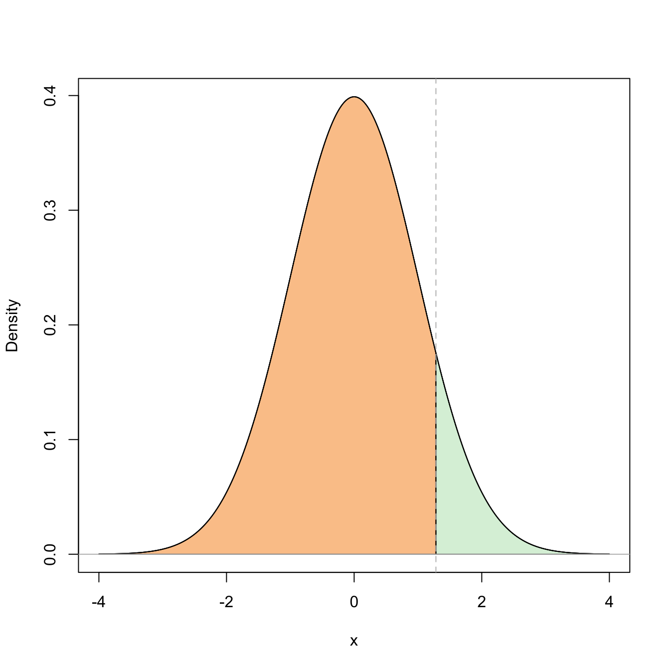
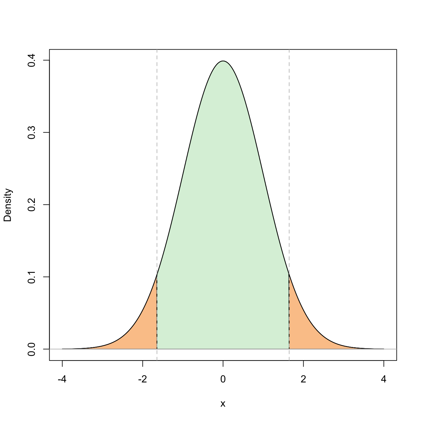
Figure 2.4: Graphical representation of the probabilities \(\mathbb{P}(Z\leq z_{\alpha/2})=1-\alpha\) and \(\mathbb{P}(-z_{\alpha/2}\leq Z\leq z_{\alpha/2})=1-\alpha\) (in green) and their complementaries (in orange) for \(\alpha=0.10\).

Setting \(\alpha=0.05,\) we can easily compute \(z_{0.025}\approx 1.96\) in R through the qnorm() function:

alpha <- 0.05
qnorm(1 - alpha / 2) # LOWER (1 - beta)-quantile = UPPER beta-quantile
## [1] 1.959964
qnorm(alpha / 2, lower.tail = FALSE) # Alternatively, lower.tail = FALSE
## [1] 1.959964
# computes the upper quantile and lower.tail = TRUE (the default) computes the
# lower quantile

Therefore, we set \(0.32\sqrt{n}=z_{0.025}\) and solve for \(n,\) which results in

\[\begin{align*} n=\left(\frac{z_{0.025}}{0.32}\right)^2\approx 37.51. \end{align*}\]

Then, if we take \(n=38,\) we have that

\[\begin{align*} \mathbb{P}(|\bar{X}-\mu| \leq 8)>0.95. \end{align*}\]

2.2.2 Sampling distribution of the sample variance

The sample variance is given by

\[\begin{align*} S^2:=\frac{1}{n}\sum_{i=1}^n (X_i-\bar{X})^2=\frac{1}{n}\sum_{i=1}^n X_i^2-{\bar{X}}^2. \end{align*}\]

The sample quasivariance will also play a relevant role in inference. It is defined by simply replacing \(n\) with \(n-1\) in the factor of \(S^2\):²⁶

\[\begin{align*} S'^2:=\frac{1}{n-1}\sum_{i=1}^n(X_i-\bar{X})^2=\frac{n}{n-1}S^2=\frac{1}{n-1}\sum_{i=1}^n X_i^2-\frac{n}{n-1}{\bar{X}}^2. \end{align*}\]

Before establishing the sampling distributions of \(S^2\) and \(S'^2,\) we obtain in the first place their expectations. For that aim, we start by decomposing the variability of the sample with respect to its expectation \(\mu\) in the following way:

\[\begin{align*} \sum_{i=1}^n(X_i-\mu)^2=\sum_{i=1}^n(X_i-\bar{X})^2+n(\bar{X}-\mu)^2 \end{align*}\]

Taking expectations, we have

\[\begin{align*} n\sigma^2=n\mathbb{E}[S^2]+n\frac{\sigma^2}{n}, \end{align*}\]

and then, solving for the expectation,

\[\begin{align} \mathbb{E}[S^2]=\frac{(n-1)}{n}\,\sigma^2.\tag{2.5} \end{align}\]

Therefore,

\[\begin{align} \mathbb{E}[S'^2]=\frac{n}{n-1}\mathbb{E}[S^2]=\sigma^2.\tag{2.6} \end{align}\]

Recall that this computation does not employ the assumption of sample normality, hence it is a general fact for \(S^2\) and \(S'^2\) irrespective of the underlying distribution. It also shows that \(S^2\) is not “pointing” towards \(\sigma^2\) but to a slightly smaller quantity, whereas \(S'^2\) is “pointing” directly to \(\sigma^2.\) This observation is related with the bias of an estimator and will be treated in detail in Section 3.1.

In order to compute the sampling distributions of \(S^2\) and \(S'^2,\) it is required to obtain the sampling distribution of the statistic \(\sum_{i=1}^n X_i^2\) when the sample is generated from a \(\mathcal{N}(0,1),\) which will follow a chi-square distribution.

Definition 2.3 (Chi-square distribution) A rv has chi-square distribution with \(\nu\in \mathbb{N}\) degrees of freedom, denoted as \(\chi_{\nu}^2,\) if its distribution coincides with the gamma distribution of shape \(\alpha=\nu/2\) and scale \(\beta=2.\)²⁷ In other words,

\[\begin{align*} \chi_{\nu}^2\stackrel{d}{=}\Gamma(\nu/2,2), \end{align*}\]

with pdf given by

\[\begin{align*} f(x;\nu)=\frac{1}{\Gamma(\nu/2) 2^{\nu/2}}\, x^{\nu/2-1} e^{-x/2}, \quad x>0, \ \nu\in\mathbb{N}. \end{align*}\]

The mean and the variance of a chi-square with \(\nu\) degrees of freedom are²⁸

\[\begin{align} \mathbb{E}[\chi_{\nu}^2]=\nu, \quad \mathbb{V}\mathrm{ar}[\chi_{\nu}^2]=2\nu. \tag{2.7} \end{align}\]

We can observe that a chi-square rv, as any gamma rv, is always positive. Also, their expectation and variance grow accordingly to the degrees of freedom \(\nu.\) When \(\nu\geq 2,\) the pdf attains its global maximum at \(\nu-2.\) If \(\nu=1\) or \(\nu=2,\) the pdf is monotone decreasing. These facts are illustrated in Figure 2.5.

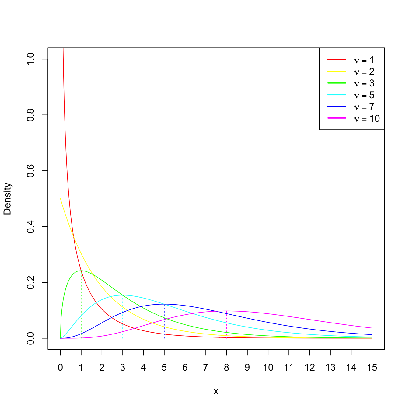
Figure 2.5: \(\chi^2_\nu\) densities for several degrees of freedom \(\nu.\) The dotted lines represent the unique modes of the densities.

The next two propositions are key for obtaining the sampling distribution of \(\sum_{i=1}^n X_i^2,\) given in Corollary 2.1.

Proposition 2.1 If \(X\sim \mathcal{N}(0,1),\) then \(X^2\sim \chi_1^2.\)

Proof (Proof of Proposition 2.1). Rather than using transformations of the pdf, we compute the cdf of the rv \(X^2.\) Since \(X\sim \mathcal{N}(0,1)\) has a symmetric pdf, then

\[\begin{align*} F_{X^2}(y) &=\mathbb{P}_{X^2}(X^2\leq y)=\mathbb{P}\left(-\sqrt{y}\leq X \leq\sqrt{y}\right)=2\mathbb{P}\left(0\leq X \leq \sqrt{y}\right)\\ &=2\int_{0}^{\sqrt{y}} \frac{1}{\sqrt{2\pi}} e^{x^2/2}\,\mathrm{d}x =\int_{0}^y \frac{1}{\sqrt{2\pi}} e^{-u/2} u^{-1/2} \,\mathrm{d}u\\ &=F_{\Gamma(1/2,2)}(y)=F_{\chi^2_1}(y), \; y>0. \end{align*}\]

Proposition 2.2 (Additive property of the chi-square) If \(X_1\sim \chi_n^2\) and \(X_2\sim \chi_m^2\) are independent, then

\[\begin{align*} X_1+X_2\sim \chi_{n+m}^2. \end{align*}\]

Proof (Proof of Proposition 2.2). The chi-square distribution is a particular case of the gamma, so the proof follows immediately using Exercise 1.21.

Corollary 2.1 Let \(X_1,\ldots,X_n\) be independent rv’s distributed as \(\mathcal{N}(0,1).\) Then,

\[\begin{align*} \sum_{i=1}^n X_i^2\sim \chi_n^2. \end{align*}\]

Proof. The proof follows directly from Propositions 2.1 and 2.2.

The last result is sometimes employed for directly defining the chi-square rv with \(\nu\) degrees of freedom as the sum of \(\nu\) independent squared \(\mathcal{N}(0,1)\) rv’s. In this way, the degrees of freedom represent the number of terms in the sum.

Example 2.9 If \((Z_1,\ldots,Z_6)\) is a srs of a standard normal, find a number \(b\) such that

\[\begin{align*} \mathbb{P}\left(\sum_{i=1}^6 Z_i^2\leq b\right)=0.95. \end{align*}\]

We know from Corollary 2.1 that

\[\begin{align*} \sum_{i=1}^6 Z_i^2\sim \chi_6^2. \end{align*}\]

Then, \(b\approx 12.59\) corresponds to the upper \(\alpha\)-quantile of a \(\chi^2_{\nu},\) denoted as \(\chi^2_{\nu;\alpha}.\) Here, \(\alpha=0.05\) and \(\nu=6.\) The quantiles \(\chi^2_{6;0.05}\) can be computed by calling the qchisq() function in R:

alpha <- 0.05
qchisq(1 - alpha, df = 6) # df stands for the degrees of freedom
## [1] 12.59159
qchisq(alpha, df = 6, lower.tail = FALSE) # Alternatively
## [1] 12.59159

The final result of this section is the famous Fisher’s Theorem, which delivers the sampling distribution of \(S^2\) and \(S'^2,\) and their independence²⁹ with respect to \(\bar{X}.\)

Theorem 2.2 (Fisher's Theorem) If \((X_1,\ldots,X_n)\) is a srs of a \(\mathcal{N}(\mu,\sigma^2)\) rv, then \(S^2\) and \(\bar{X}\) are independent, and

\[\begin{align*} \frac{nS^2}{\sigma^2}=\frac{(n-1)S'^2}{\sigma^2}\sim\chi_{n-1}^2. \end{align*}\]

Proof (Proof of Theorem 2.2). We apply Theorem 2.6 given in the Appendix for \(p=1,\) in such a way that

\[\begin{align*} nS^2=\sum_{i=1}^n X_i^2-(\sqrt{n}\bar{X})^2=\sum_{i=1}^n X_i^2-\boldsymbol{c}_1^\top X, \end{align*}\]

for \(\boldsymbol{c}_1=(1/\sqrt{n},\ldots,1/\sqrt{n})^\top\) and \(\boldsymbol{X}=(X_1,\ldots,X_n)^\top.\) Therefore, by such theorem, \(S^2\) is independent of \(\bar{X},\) and \(\frac{nS^2}{\sigma^2}\sim \chi_{n-1}^2.\)

Example 2.10 Assume that we have a srs made of 10 bottles from the filling machine of Example 2.7 where \(\sigma^2=625.\) Find a pair of values \(b_1\) and \(b_2\) such that

\[\begin{align*} \mathbb{P}(b_1\leq S'^2\leq b_2)=0.90. \end{align*}\]

We know from Theorem 2.2 that \(\frac{(n-1)S'^2}{\sigma^2}\sim\chi_{n-1}^2.\) Therefore, multiplying by \((n-1)\) and dividing by \(\sigma^2\) in the previous probability, we get

\[\begin{align*} \mathbb{P}(b_1\leq S'^2\leq b_2)&=\mathbb{P}\left(\frac{(n-1)b_1}{\sigma^2}\leq \frac{(n-1)S'^2}{\sigma^2} \leq \frac{(n-1)b_2}{\sigma^2}\right)\\ &=\mathbb{P}\left(\frac{9b_1}{625}\leq \chi_9^2 \leq \frac{9b_2}{625}\right). \end{align*}\]

Set \(a_1=\frac{9b_1}{625}\) and \(a_2=\frac{9b_2}{625}.\) A possibility is to select:

• \(a_1\) such that the cumulative probability to its left (right) is \(0.05\) (\(0.95\)). This corresponds to the upper \((1-\alpha/2)\)-quantile, \(\chi^2_{\nu;1-\alpha/2},\) with \(\alpha=0.10\) (because \(1-\alpha=0.90\)).
• \(a_2\) such that the cumulative probability to its right is \(0.05.\) This corresponds to the upper \(\alpha/2\)-quantile, \(\chi^2_{\nu;\alpha/2}.\)

Recall that, unlike in the situation of Example 2.8, the pdf of a chi-square is not symmetric, and hence \(\chi^2_{\nu;1-\alpha}\neq -\chi^2_{\nu;\alpha}\) (for the normal we had that \(z_{1-\alpha}= -z_{\alpha}\) and therefore we only cared about \(z_{\alpha}\)).

We can compute \(a_1=\chi^2_{9;0.95}\) and \(a_2=\chi^2_{9;0.05}\) by employing the function qchisq():

alpha <- 0.10
qchisq(1 - alpha / 2, df = 9, lower.tail = FALSE) # a1
## [1] 3.325113
qchisq(alpha / 2, df = 9, lower.tail = FALSE) # a2
## [1] 16.91898

Then, \(a_1\approx3.325\) and \(a_2\approx16.919,\) so the asked values are \(b_1\approx3.325\times 625/9=230.903\) and \(b_2\approx 16.919\times 625 / 9=1174.931.\)

2.2.3 Student’s \(t\) distribution

Definition 2.4 (Student’s \(t\) distribution) Let \(X\sim \mathcal{N}(0,1)\) and \(Y\sim \chi_{\nu}^2\) be independent rv’s. The distribution of the rv

\[\begin{align*} T=\frac{X}{\sqrt{Y/\nu}} \end{align*}\]

is the Student’s \(t\) distribution with \(\nu\) degrees of freedom.³⁰

The pdf of the Student’s \(t\) distribution is (see the Exercise 2.22)

\[\begin{align*} f(t;\nu)=\frac{\Gamma\left(\frac{\nu+1}{2}\right)}{\sqrt{\nu \pi}\,\Gamma\left(\frac{\nu}{2}\right)}\left(1+\frac{t^2}{\nu}\right)^{-(\nu+1)/2},\quad t\in \mathbb{R}. \end{align*}\]

We can see that the density is symmetric with respect to zero. When \(\nu>1,\)³¹ its expectation is \(\mathbb{E}[T]=0\) and, when \(\nu>2,\) its variance is \(\mathbb{V}\mathrm{ar}[T]=\nu/(\nu-2)>1.\) This means that for \(\nu>2,\) \(T\) has a larger variability than the standard normal. However, the differences between a \(t_{\nu}\) and a \(\mathcal{N}(0,1)\) vanish as \(\nu\to\infty,\) as it can be seen in Figure 2.6.

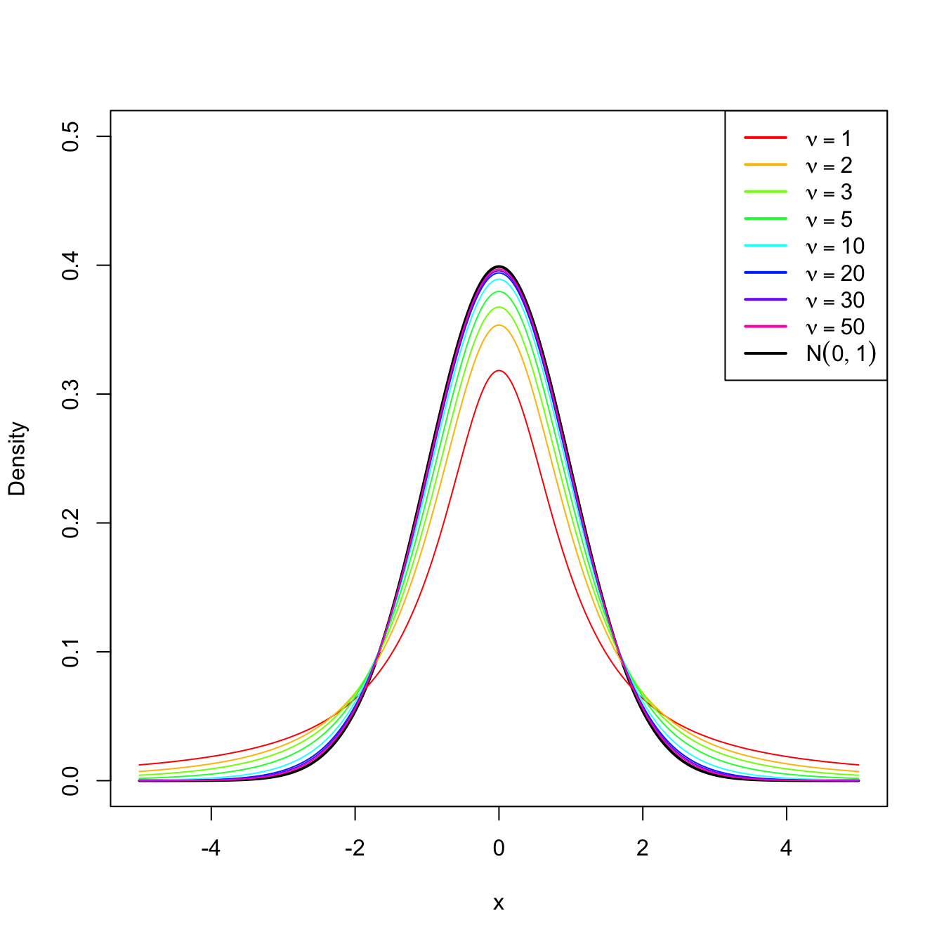
Figure 2.6: \(t_\nu\) densities for several degrees of freedom \(\nu.\) Observe the convergence to a \(\mathcal{N}(0,1)\) as \(\nu\to\infty.\)

Theorem 2.3 (Student's Theorem) Let \((X_1,\ldots,X_n)\) be a srs of a \(\mathcal{N}(\mu,\sigma^2)\) rv. Let \(\bar{X}\) and \(S'^2\) be the sample mean and quasivariance, respectively. Then,

\[\begin{align*} T=\frac{\bar{X}-\mu}{S'/\sqrt{n}}\sim t_{n-1}. \end{align*}\]

and the statistic \(T\) is referred to as the (Student’s) \(T\) statistic.

Proof (Proof of Theorem 2.3). From Theorem 2.1, we can deduce that

\[\begin{align} \frac{\bar{X}-\mu}{\sigma/\sqrt{n}}\sim \mathcal{N}(0,1).\tag{2.8} \end{align}\]

On the other hand, by Theorem 2.2 we know that

\[\begin{align} \frac{(n-1)S'^2}{\sigma^2}\sim \chi_{n-1}^2,\tag{2.9} \end{align}\]

and that (2.9) is independent of (2.8). Therefore, dividing (2.8) by the square root of (2.9) divided by its degrees of freedom, we obtain a rv with Student’s \(t\) distribution:

\[\begin{align*} T=\frac{\sqrt{n}\, \frac{\bar{X}-\mu}{\sigma}}{\sqrt{\frac{(n-1)S'^2}{\sigma^2}/(n-1)}}=\frac{\bar{X}-\mu}{S'/\sqrt{n}}\sim t_{n-1}. \end{align*}\]

Example 2.11 The resistance to electric tension of a certain kind of wire is distributed according to a normal with mean \(\mu\) and variance \(\sigma^2,\) both unknown. Six segments of the wire are selected at random and their resistances are measured, resulting in \(X_1,\ldots,X_6.\) Find the approximate probability that the difference between \(\bar{X}\) and \(\mu\) is less than \(2S'/\sqrt{n}\) units.

We want to compute the probability

\[\begin{align*} \mathbb{P}&\left(-\frac{2S'}{\sqrt{n}}\leq \bar{X}-\mu\leq\frac{2S'}{\sqrt{n}}\right)=\mathbb{P}\left(-2\leq \sqrt{n}\frac{\bar{X}-\mu}{S'}\leq 2\right)\\ &\quad=\mathbb{P}(-2\leq T\leq 2)=1-2\mathbb{P}(T\leq -2). \end{align*}\]

From Theorem 2.3, we know that \(T\sim t_5.\) The probabilities \(\mathbb{P}(t_\nu\leq x)\) can be computed with pt(x, df = nu):

pt(-2, df = 5)
## [1] 0.05096974

Therefore, the probability is approximately \(1-2\times 0.051=0.898.\)

2.2.4 Snedecor’s \(\mathcal{F}\) distribution

Definition 2.5 (Snedecor’s \(\mathcal{F}\) distribution) Let \(X_1\) and \(X_2\) be chi-square rv’s with \(\nu_1\) and \(\nu_2\) degrees of freedom, respectively. If \(X_1\) and \(X_2\) are independent, then the rv

\[\begin{align*} F=\frac{X_1/\nu_1}{X_2/\nu_2} \end{align*}\]

is said to have an Snedecor’s \(\mathcal{F}\) distribution with \(\nu_1\) and \(\nu_2\) degrees of freedom, which is represented as \(\mathcal{F}_{\nu_1,\nu_2}.\)

Remark. It can be seen that \(\mathcal{F}_{1,\nu}\) coincides with \(t_{\nu}^2.\)

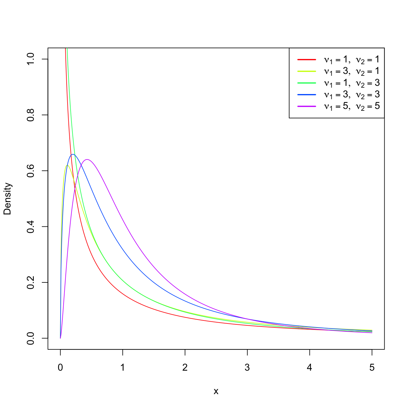
Figure 2.7: \(\mathcal{F}_{\nu_1,\nu_2}\) densities for several degrees of freedom \(\nu_1\) and \(\nu_2.\)

Theorem 2.4 (Sampling distribution of the ratio of quasivariances) Let \((X_1,\ldots,X_{n_1})\) be a srs from a \(\mathcal{N}(\mu_1,\sigma_1^2)\) and let \(S_1'^2\) be its sample quasivariance. Let \((Y_1,\ldots,Y_{n_2})\) be another srs, independent from the previous one, from a \(\mathcal{N}(\mu_2,\sigma_2^2)\) and with sample quasivariance \(S_2'^2.\) Then,

\[\begin{align*} F=\frac{S_1'^2/\sigma_1^2}{S_2'^2/\sigma_2^2}\sim\mathcal{F}_{n_1-1,n_2-1}. \end{align*}\]

Proof (Proof of Theorem 2.4). The proof is straightforward from the independence of both samples, the application of Theorem 2.2 and the definition of Snedecor’s \(\mathcal{F}\) distribution, since

\[\begin{align*} F=\frac{\frac{(n_1-1)S_1'^2}{\sigma_1^2}/(n_1-1)}{\frac{(n_2-1)S_2'^2}{\sigma_2^2}/(n_2-1)}=\frac{S_1'^2/\sigma_1^2}{S_2'^2/\sigma_2^2}\sim\mathcal{F}_{n_1-1,n_2-1}. \end{align*}\]

Example 2.12 If we take two independent srs’s of sizes \(n_1=6\) and \(n_2=10\) from two normal populations with the same (but unknown) variance \(\sigma^2,\) find the number \(b\) such that

\[\begin{align*} \mathbb{P}\left(\frac{S_1'^2}{S_2'^2}\leq b\right)=0.95. \end{align*}\]

We have that

\[\begin{align*} \mathbb{P}\left(\frac{S_1'^2}{S_2'^2}\leq b\right)=0.95\iff \mathbb{P}\left(\frac{S_1'^2}{S_2'^2}> b\right)=0.05. \end{align*}\]

By Theorem 2.4, we know that

\[\begin{align*} \frac{S_1'^2/\sigma_1^2}{S_2'^2/\sigma_2^2}=\frac{S_1'^2}{S_2'^2}\sim\mathcal{F}_{5,9}. \end{align*}\]

Therefore, we look for the upper \(\alpha\)-quantile \(\mathcal{F}_{\nu_1,\nu_2;\alpha}\) such that \(\mathbb{P}(\mathcal{F}_{\nu_1,\nu_2}>\mathcal{F}_{\nu_1,\nu_2;\alpha})=\alpha,\) for \(\alpha=0.05,\) \(\nu_1=5,\) and \(\nu_2=9.\) This can be obtained with the function qf(), which provides \(b=:\mathcal{F}_{5,9;0.05}\):

qf(0.05, df1 = 5, df2 = 9, lower.tail = FALSE)
## [1] 3.481659

2.3 The central limit theorem

The Central Limit Theorem (CLT) is a cornerstone result in statistics, if not the cornerstone result. The result states that the sampling distribution of the sample mean \(\bar{X}\) of iid rv’s \(X_1,\ldots,X_n\) converges to a normal distribution as \(n\to\infty.\) The beauty of this result is that it holds irrespective of the original distribution of \(X_1,\ldots,X_n.\)

Theorem 2.5 (Central limit theorem) Let \(X_1,\ldots,X_n\) be iid rv’s with expectation \(\mathbb{E}[X_i]=\mu\) and variance \(\mathbb{V}\mathrm{ar}[X_i]=\sigma^2<\infty.\) Then, the cdf of the rv

\[\begin{align*} U_n=\frac{\bar{X}-\mu}{\sigma/\sqrt{n}} \end{align*}\]

converges to the cdf of a \(\mathcal{N}(0,1)\) as \(n\to\infty.\)

Remark. To denote “approximately distributed as” we will use \(\cong.\) We can therefore write that, due to the CLT, \(\frac{\bar{X}-\mu}{\sigma/\sqrt{n}}\cong \mathcal{N}(0,1)\) (as \(n\to\infty\)). Observe that this notation is different from \(\sim,\) used to denote “distributed as”, or \(\approx,\) used for approximations of numerical quantities.

Proof (Proof of Theorem 2.5). We compute the mgf of the rv \(U_n.\) Since \(X_1,\ldots,X_n\) are independent,

\[\begin{align*} M_{U_n}(s)&=\mathbb{E}\left[\exp\left\{s U_n\right\}\right]=\mathbb{E}\left[ \exp\left\{s\sum_{i=1}^n\left(\frac{X_i-\mu}{\sigma\sqrt{n}}\right) \right\}\right]\\ &=\prod_{i=1}^n \mathbb{E}\left[\exp\left\{s\, \frac{X_i -\mu}{\sigma\sqrt{n}}\right\}\right]. \end{align*}\]

Now, denoting \(Z:=(X_1-\mu)/\sigma\) (this variable is standardized but it is not a standard normal variable), we have

\[\begin{align*} M_{U_n}(s)&=\left(\mathbb{E}\left[\exp\left\{\frac{s}{\sqrt{n}} Z\right\}\right]\right)^n=\left[M_Z\left(\frac{s}{\sqrt{n}}\right)\right]^n, \end{align*}\]

The rv \(Z\) is such that \(\mathbb{E}[Z]=0\) and \(\mathbb{E}[Z^2]=1.\) We perform a second-order Taylor expansion of \(M_Z(s/\sqrt{n})\) about \(s=0\):

\[\begin{align*} M_Z\left(\frac{s}{\sqrt{n}}\right)=M_Z(0)+M_Z^{(1)}(0)\frac{\left(s/\sqrt{n}\right)}{1!}+M_Z^{(2)}(0)\frac{\left(s/\sqrt{n}\right)^2}{2!}+R(s/\sqrt{n}), \end{align*}\]

where \(M_Z^{(k)}(0)\) is the \(k\)-th derivative of the mgf evaluated at \(s=0\) and the remainder term \(R\) is a function that satisfies

\[\begin{align*} \lim_{n\to\infty} \frac{R\left(s/\sqrt{n}\right)}{(s/\sqrt{n})^2}=0, \end{align*}\]

i.e., its contribution in the Taylor expansion is negligible in comparison with the second term \((s/\sqrt{n})^2\) when \(n\to\infty.\)

Since the derivatives evaluated at zero are equal to the moments (Theorem 1.1), we have:

\[\begin{align*} M_Z\left(\frac{s}{\sqrt{n}}\right) &=\mathbb{E}\left[e^0\right]+\mathbb{E}[Z]\frac{s}{\sqrt{n}}+\mathbb{E}\left[Z^2\right]\frac{s^2}{2n}+R\left(\frac{s}{\sqrt{n}}\right) \\ &=1+\frac{s^2}{2n}+R\left(\frac{s}{\sqrt{n}}\right) \\ &=1+\frac{1}{n}\left[\frac{s^2}{2}+nR\left(\frac{s}{\sqrt{n}}\right)\right]. \end{align*}\]

Now,

\[\begin{align*} \lim_{n\to\infty} M_{U_n}(s)&=\lim_{n\to\infty}\left[M_Z\left(\frac{s}{\sqrt{n}}\right)\right]^n\\ &=\lim_{n\to\infty}\left\{1+\frac{1}{n}\left[\frac{s^2}{2}+nR\left(\frac{s}{\sqrt{n}}\right)\right]\right\}^n. \end{align*}\]

In order to compute the limit, we use that, as \(x\to0,\) \(\log(1+x)=x+L(x)\) with remainder \(L\) such that \(\lim_{x\to 0} L(x)/x=0.\) Then,

\[\begin{align} \lim_{n\to\infty}nR\left(\frac{s}{\sqrt{n}}\right)&=\lim_{n\to\infty} s^2 \frac{R(s/\sqrt{n})}{(s/\sqrt{n})^2}=0,\tag{2.10}\\ \lim_{n\to\infty} nL\left(\frac{s^2}{2n}\right)&=\lim_{n\to\infty}\frac{2}{s^2}\frac{L\left(s^2/(2n)\right)}{s^2/(2n)}=0.\tag{2.11} \end{align}\]

Then, applying the logarithm and using its expansion plus (2.10) and (2.11), we have

\[\begin{align*} \lim_{n\to\infty} \log M_{U_n}(s)&=\lim_{n\to\infty}n\log\left\{1+\frac{1}{n}\left[\frac{s^2}{2}+nR\left(\frac{s}{\sqrt{n}}\right)\right]\right\}\\ &=\lim_{n\to\infty}n \left\{\frac{1}{n}\left[\frac{s^2}{2}+nR\left(\frac{s}{\sqrt{n}}\right)\right]+L\left(\frac{s^2}{2n}\right)\right\}\\ &=\frac{s^2}{2}+\lim_{n\to\infty} nR\left(\frac{s}{\sqrt{n}}\right)+\lim_{n\to\infty} nL\left(\frac{s^2}{2n}\right)\\ &=\frac{s^2}{2}. \end{align*}\]

Therefore,

\[\begin{align*} \lim_{n\to\infty}M_{U_n}(s)=e^{s^2/2}=M_{\mathcal{N}(0,1)}(s), \end{align*}\]

where \(M_{\mathcal{N}(0,1)}(s)=e^{s^2/2}\) is seen in Exercise 1.18.

The application of Theorem 1.3 ends the proof.

Remark. If \(X_1,\ldots,X_n\) are normal rv’s, then \(U_n\) is exactly distributed as \(\mathcal{N}(0,1).\) This is the exact version of the CLT.

Example 2.13 The grades in a first-year course of a given university have a mean of \(\mu=6.1\) points (over \(10\) points) and a standard deviation of \(\sigma=1.5,\) both known from long-term records. A specific generation of \(n=38\) students had a mean of \(5.5\) points. Can we state that these students have a significantly lower performance? Or perhaps this is a reasonable deviation from the average performance merely due to randomness? In order to answer, compute the probability that the sample mean is at most \(5.5\) when \(n=38.\)

Let \(\bar{X}\) be the sample mean of the srs of \(n=38\) students grades. By the CLT we know that

\[\begin{align*} Z=\frac{\bar{X}-\mu}{\sigma/\sqrt{n}}\cong \mathcal{N}(0,1). \end{align*}\]

Then, we are interested in computing the probability

\[\begin{align*} \mathbb{P}(\bar{X}\leq 5.5)=\mathbb{P}\left(Z\leq \frac{5.5-6.1}{1.5/\sqrt{38}}\right)\approx\mathbb{P}(Z\leq -2.4658)\approx 0.0068, \end{align*}\]

which has been obtained with

pnorm(-2.4658)
## [1] 0.006835382
pnorm(5.5, mean = 6.1, sd = 1.5 / sqrt(38)) # Alternatively
## [1] 0.006836039

Observe that this probability is very small. This suggests that it is highly unlikely that this generation of students belongs to the population with mean \(\mu=6.1.\) It is more likely that its true mean is smaller than \(6.1\) and therefore the generation of current students has a significantly lower performance than previous generations.

Example 2.14 The random waiting time in a cash register of a supermarket is distributed according to a distribution with mean \(1.5\) minutes and variance \(1.\) What is the approximate probability of serving \(n=100\) clients in less than \(2\) hours?

If \(X_i\) denotes the waiting time of the \(i\)-th client, then we want to compute

\[\begin{align*} \mathbb{P}\left(\sum_{i=1}^{100} X_i\leq 120\right)=\mathbb{P}\left(\bar{X}\leq 1.2\right). \end{align*}\]

As the sample size is large, the CLT entails that \(\bar{X}\cong\mathcal{N}(1.5, 1/100),\) so

\[\begin{align*} \mathbb{P}\left(\bar{X}\leq 1.2\right)=\mathbb{P}\left(\frac{\bar{X}-1.5}{1/\sqrt{100}} \leq \frac{1.2-1.5}{1/\sqrt{100}}\right)\approx \mathbb{P}(Z\leq -3). \end{align*}\]

Employing pnorm() we can compute \(\mathbb{P}(Z\leq -3)\) right away:

pnorm(-3)
## [1] 0.001349898

The CLT employs a type of convergence for sequences of rv’s that we precise next.

Definition 2.6 (Convergence in distribution) A sequence of rv’s \(X_1,X_2,\ldots\) converges in distribution to a rv \(X\) if

\[\begin{align*} \lim_{n\to\infty} F_{X_n}(x)=F_X(x), \end{align*}\]

for all the points \(x\in\mathbb{R}\) where \(F_X(x)\) is continuous. The convergence in distribution is denoted by

\[\begin{align*} X_n \stackrel{d}{\longrightarrow} X. \end{align*}\]

The thesis of the CLT can be rewritten in terms of this (more explicit) notation as follows:

\[\begin{align*} U_n=\frac{\bar{X}-\mu}{\sigma/\sqrt{n}}\stackrel{d}{\longrightarrow}\mathcal{N}(0,1). \end{align*}\]

This means that the cdf of \(U_n,\) \(F_{U_n},\) verifies that \(\lim_{n\to\infty} F_{U_n}(x)=\Phi(x)\) for all \(x\in\mathbb{R}.\) We can visualize how this convergence happens by plotting the cdf’s of \(U_n\) for increasing values of \(n\) and matching them with \(\Phi,\) the cdf of a standard normal. This is done in Figures 2.8 and 2.9, where the cdf’s \(F_{U_n}\) are approximated by Monte Carlo.

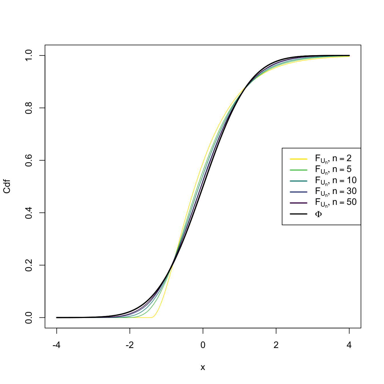
Figure 2.8: Cdf’s of \(U_n=(\bar{X}-\mu)/(\sigma/\sqrt{n})\) for \(X_1,\ldots,X_n\sim \mathrm{Exp}(2).\) A fast convergence of \(F_{U_n}\) towards \(\Phi\) appears, despite the heavy non-normality of \(\mathrm{Exp}(2)\).

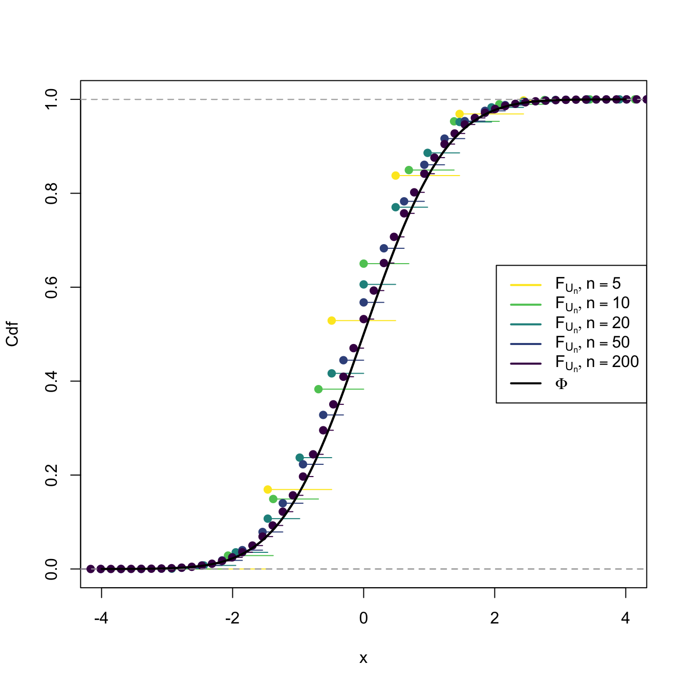
Figure 2.9: Cdf’s of \(U_n=(\bar{X}-\mu)/(\sigma/\sqrt{n})\) for \(X_1,\ldots,X_n\sim \mathrm{Bin}(1,p).\) The cdf’s \(F_{U_n}\) are discrete for every \(n,\) which makes their convergence towards \(\Phi\) slower than in the continuous case.

The diagram below summarizes the available sampling distributions for the sample mean:

\[\begin{align*} \!\!\!\!\!\!\!\!(X_1,\ldots,X_n)\begin{cases} \sim \mathcal{N}(\mu,\sigma^2) & \implies \bar{X}\sim \mathcal{N}(\mu,\sigma^2/n) \\ \nsim \mathcal{N}(\mu,\sigma^2) & \begin{cases} n \;\text{ small} & \implies \text{?} \\ n \;\text{ large} & \implies \bar{X}\cong \mathcal{N}(\mu,\sigma^2/n) \end{cases} \end{cases} \end{align*}\]

The following examples provide another view on the applicability of the CLT: to approximate certain distributions for large values of their parameters.

Example 2.15 (Normal approximation to the binomial) Let \(Y\) be a binomial rv of size \(n\in\mathbb{N}\) and success probability \(p\in[0,1]\) (see Example 1.22), denoted by \(\mathrm{Bin}(n,p).\) It holds that \(Y=\sum_{i=1}^n X_i,\) where \(X_i\sim \mathrm{Ber}(p),\) \(i=1,\ldots,n,\) with \(\mathrm{Ber}(p)\stackrel{d}{=}\mathrm{Bin}(1,p)\) and \(X_1,\ldots,X_n\) independent.

It is easy to see that

\[\begin{align*} \mathbb{E}[X_i]=p, \quad \mathbb{V}\mathrm{ar}[X_i]=p(1-p). \end{align*}\]

Then, applying the CLT, we have that

\[\begin{align*} \bar{X}=\frac{Y}{n}\cong \mathcal{N}\left(p,\frac{p(1-p)}{n}\right), \end{align*}\]

which implies that \(\mathrm{Bin}(n,p)/n\cong \mathcal{N}\left(p,\frac{p(1-p)}{n}\right),\) or, equivalently,

\[\begin{align} \mathrm{Bin}(n,p)\cong \mathcal{N}(np,np(1-p)) \tag{2.12} \end{align}\]

as \(n\to\infty.\) This approximation works well even when \(n\) is not very large (i.e., \(n<30\)), as long as \(p\) is “not very close to zero or one”, which is often translated as requiring that both \(np>5\) and \(np(1-p)>5\) hold.

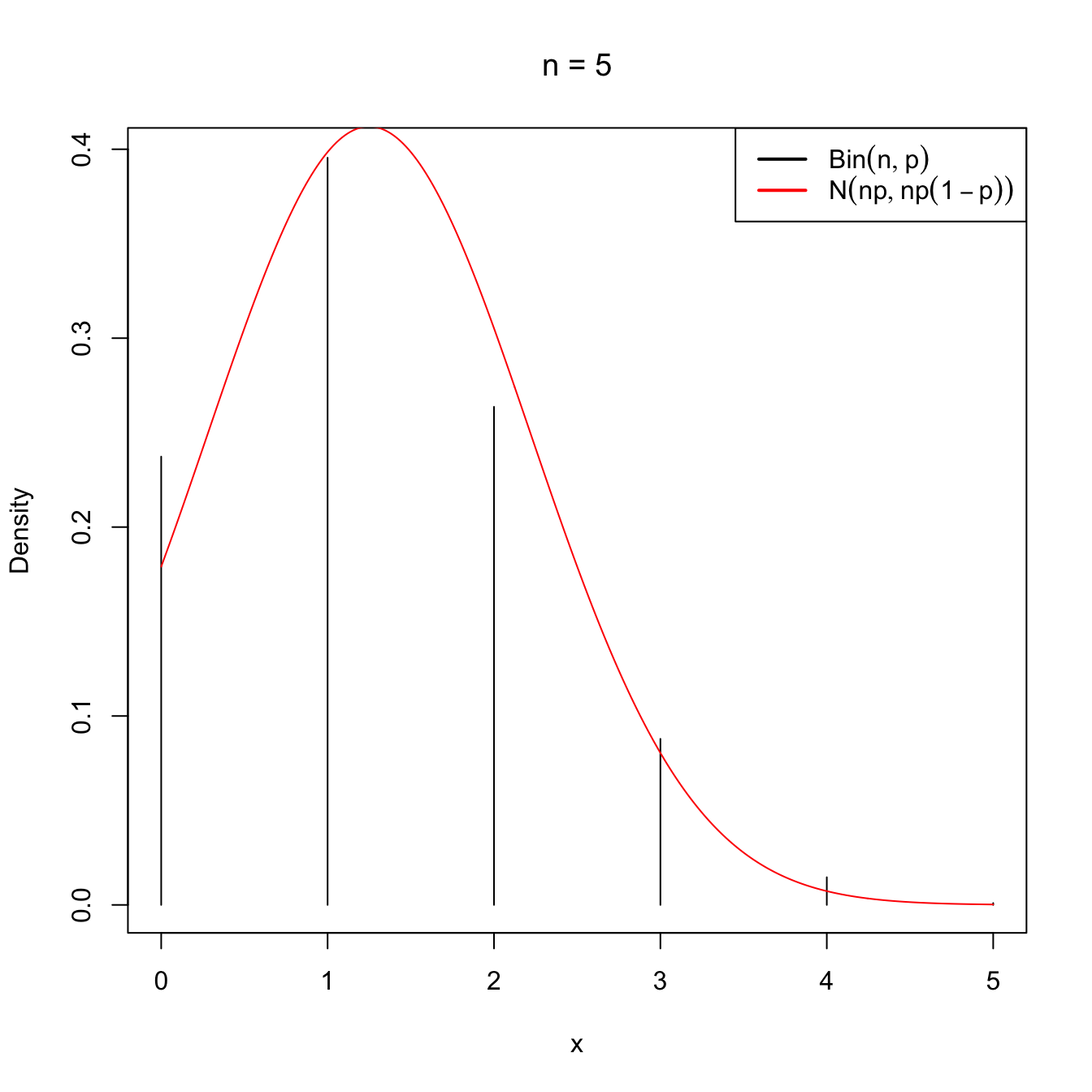
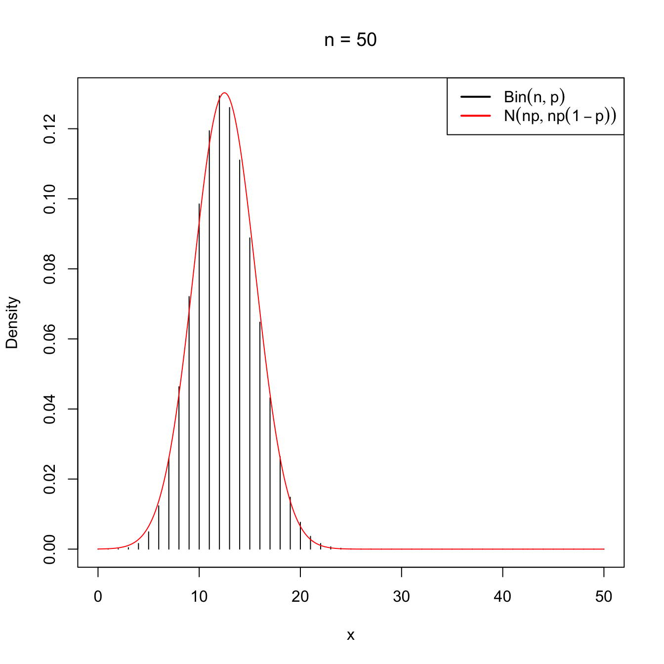
Figure 2.10: Normal approximation to the \(\mathrm{Bin}(n,p)\) for \(n=5\) and \(n=50\) with \(p=0.25\).

A continuity correction is often employed for improving the accuracy in the computation of binomial probabilities. Then, if \(\tilde{Y}\sim\mathcal{N}(np,np(1-p))\) denotes the approximating rv, better approximations are obtained with

\[\begin{align*} \mathbb{P}(Y\leq m) & \approx \mathbb{P}(\tilde{Y}\leq m+0.5), \\ \mathbb{P}(Y\geq m) & \approx \mathbb{P}(\tilde{Y}\geq m-0.5), \\ \mathbb{P}(Y=m) & \approx \mathbb{P}(m-0.5\leq \tilde{Y}\leq m+0.5), \end{align*}\]

where \(m\in\mathbb{N}\) and \(m\leq n.\)

Example 2.16 Let \(Y\sim\mathrm{Bin}(25,0.4).\) Using the normal distribution, approximate the probability that \(Y\leq 8\) and that \(Y=8.\)

Using the continuity correction, \(\mathbb{P}(Y\leq 8)\) can be approximated as

\[\begin{align*} \mathbb{P}(Y\leq 8)\approx \mathbb{P}(\tilde{Y}\leq 8.5)=\mathbb{P}(\mathcal{N}(10,6)\leq 8.5). \end{align*}\]

and its actual value is

pnorm(8.5, mean = 10, sd = sqrt(6))
## [1] 0.2701457

The probability of \(Y=8\) is approximated as

\[\begin{align*} \mathbb{P}(Y=8) \approx \mathbb{P}(7.5\leq \tilde{Y}\leq 8.5)=\mathbb{P}(7.5\leq \mathcal{N}(10,6)\leq 8.5) \end{align*}\]

and its actual value is

pnorm(8.5, mean = 10, sd = sqrt(6)) - pnorm(7.5, mean = 10, sd = sqrt(6))
## [1] 0.1164286

We can compare these two approximated probabilities with the exact ones

\[\begin{align*} \mathbb{P}(\mathrm{Bin}(n, p) \leq m) \text{ and } \mathbb{P}(\mathrm{Bin}(n, p) = m), \end{align*}\]

which can be computed right away with pbinom(m, size = n, prob = p) and dbinom(m, size = n, prob = p), respectively:

pbinom(8, size = 25, prob = 0.4)
## [1] 0.2735315
dbinom(8, size = 25, prob = 0.4)
## [1] 0.1199797

The normal approximation is therefore quite precise, even for \(n=25.\)

Example 2.17 A candidate for city mayor believes that he/she may win the elections if he/she obtains at least \(55\%\) of the votes in district D. In addition, he/she assumes that the \(50\%\) of all the voters in the city support him/her. If \(n=100\) voters vote in district D (consider them as a srs of the voters of the city), what is the exact probability that the candidate wins at least the \(55\%\) of the votes?

Let \(Y\) be the number of voters in district D that supports the candidate. \(Y\) is distributed as \(\mathrm{Bin}(100,0.5)\) and we want to know the probability

\[\begin{align*} \mathbb{P}(Y/n\geq 0.55)=\mathbb{P}(Y\geq 55). \end{align*}\]

The desired probability is

\[\begin{align*} \mathbb{P}(\mathrm{Bin}(100, 0.5) \geq 55)=1-\mathbb{P}(\mathrm{Bin}(100, 0.5) < 55), \end{align*}\]

which can be computed as:

1 - pbinom(54, size = 100, prob = 0.5)
## [1] 0.1841008
pbinom(54, size = 100, prob = 0.5, lower.tail = FALSE) # Alternatively
## [1] 0.1841008

The previous value was the exact probability for a binomial. Let us see now how close the CLT approximation is. Because of the CLT,

\[\begin{align*} \mathbb{P}(Y/n\geq 0.55)\approx\mathbb{P}\left(\mathcal{N}\left(0.5, \frac{0.25}{100}\right)\geq 0.55\right) \end{align*}\]

with the actual value given by

1 - pnorm(0.55, mean = 0.5, sd = sqrt(0.25 / 100))
## [1] 0.1586553

If the continuity correction was employed, the probability is approximated to

\[\begin{align*} \mathbb{P}(Y\geq 0.55n)\approx\mathbb{P}\left(\tilde{Y}\geq 0.55n-0.5\right)=\mathbb{P}\left(\mathcal{N}\left(50, 25\right)\geq 54.5\right), \end{align*}\]

which takes the value

1 - pnorm(54.5, mean = 50, sd = sqrt(25))
## [1] 0.1840601

As seen, the continuity correction offers a significant improvement, even for \(n=100\) and \(p=0.5.\)

Example 2.18 (Normal approximation to additive distributions) The additive property of the binomial is key for obtaining its normal approximation by the CLT seen in Example 2.15. On one hand, if \(X_1,\ldots,X_n\) are \(\mathrm{Bin}(1,p),\) then \(n\bar{X}\) is \(\mathrm{Bin}(n,p).\) On the other hand, the CLT thesis can also be expressed as

\[\begin{align} n\bar{X}\cong\mathcal{N}(n\mu,n\sigma^2) \tag{2.13} \end{align}\]

as \(n\to\infty.\) Equaling both results we have the approximation (2.12).

Different additive properties are also satisfied by other distributions, as we saw in Exercise 1.20 (Poisson distribution) and Exercise 1.21 (gamma distribution). In addition, the chi-square distribution, as a particular case of the gamma, has also an additive property (Proposition 2.2) on the degrees of freedom \(\nu.\) Therefore, we can obtain normal approximations for these distributions as well.

For the Poisson, we know that, if \((X_1,\ldots,X_n)\) is a srs of a \(\mathrm{Pois}(\lambda),\) then

\[\begin{align} n\bar{X}=\sum_{i=1}^nX_i\sim\mathrm{Pois}(n\lambda).\tag{2.14} \end{align}\]

Since the expectation and the variance of a \(\mathrm{Pois}(\lambda)\) are both equal to \(\lambda,\) equaling (2.13) and (2.14) when \(n\to\infty\) yields

\[\begin{align*} \mathrm{Pois}(n\lambda)\cong \mathcal{N}(n\lambda,n\lambda). \end{align*}\]

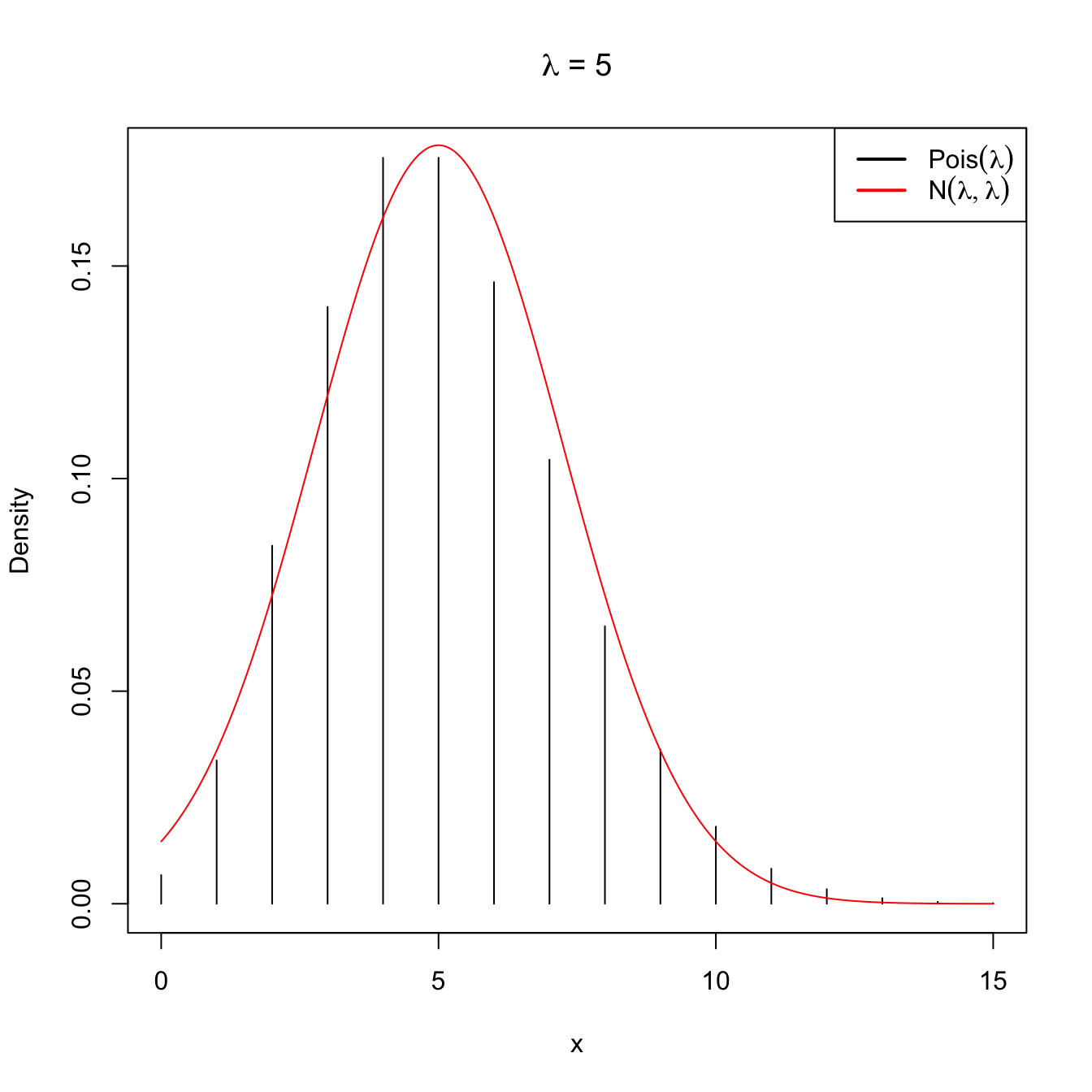
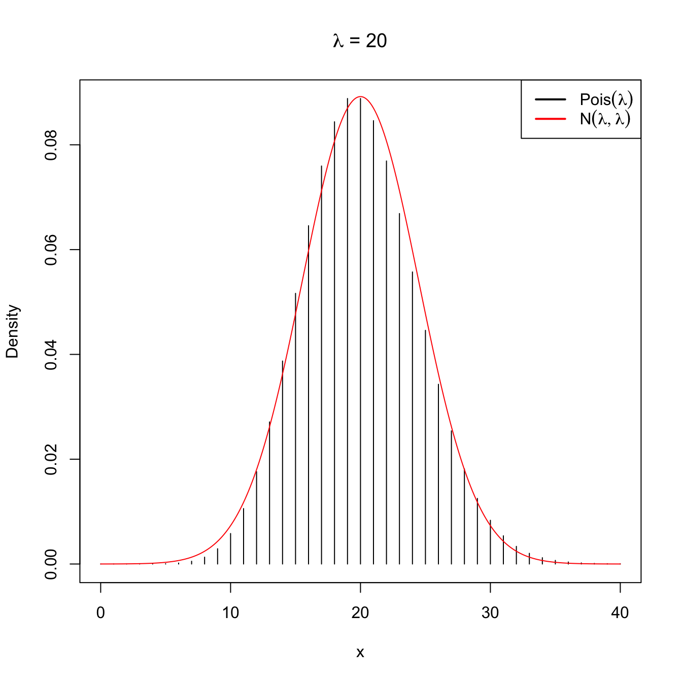
Figure 2.11: Normal approximation to the \(\mathrm{Pois}(\lambda)\) for \(\lambda=5\) and \(\lambda=20\).

Note that this approximation is equivalent to saying that when the intensity parameter \(\lambda\) tends to infinity, then \(\mathrm{Pois}(\lambda)\) is approximately a \(\mathcal{N}(\lambda,\lambda).\)

Following similar arguments for the chi-square distribution, it is easy to see that, when \(\nu\to\infty,\)

\[\begin{align} \chi^2_\nu\cong \mathcal{N}(\nu,2\nu). \tag{2.15} \end{align}\]

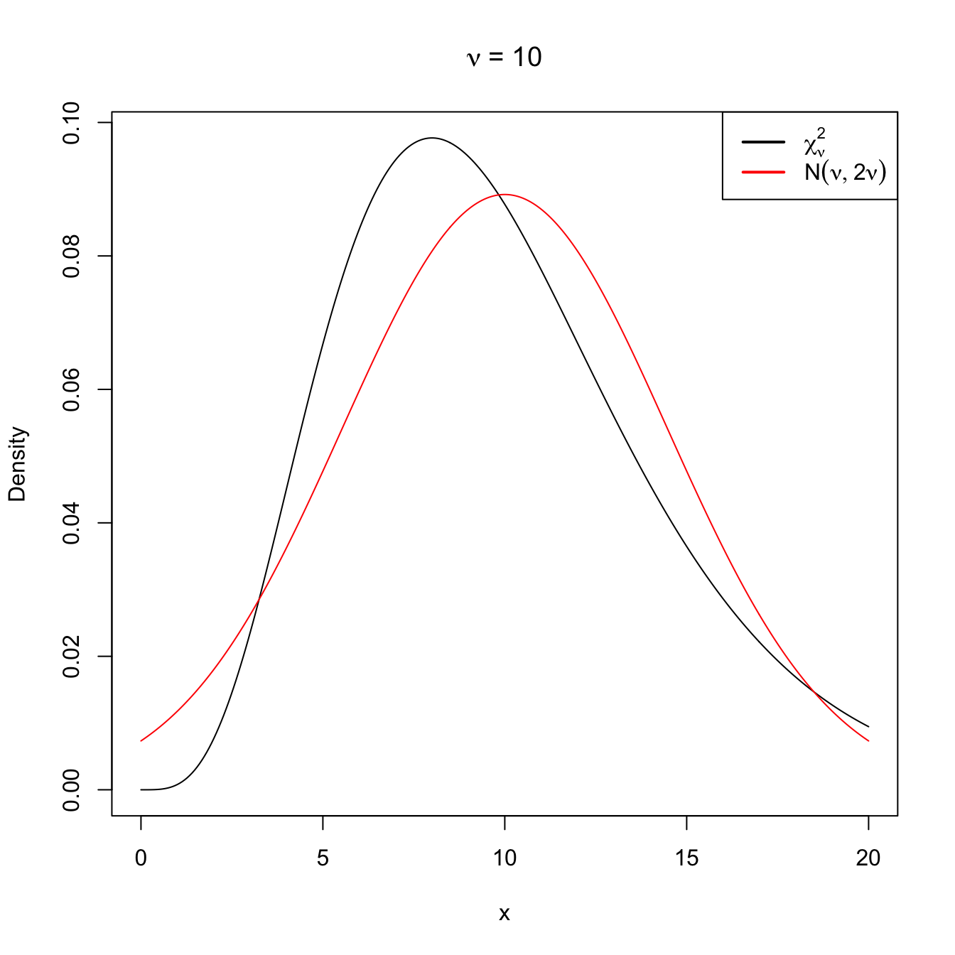
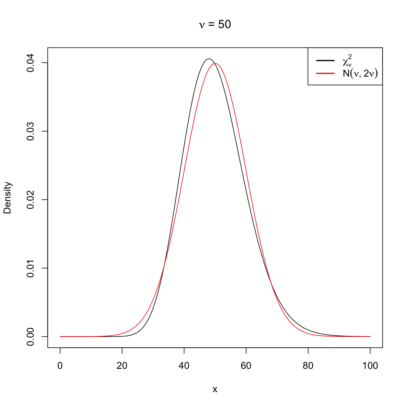
Figure 2.12: Normal approximation to the \(\chi^2_\nu\) for \(\nu=10\) and \(\nu=50\).

Appendix

The next theorem is a generalization of Fisher’s Theorem (Theorem 2.2). It is key in statistical inference.

Theorem 2.6 Let \(\boldsymbol{X}=(X_1,\ldots,X_n)^\top\) be a vector of iid rv’s distributed as \(\mathcal{N}(0,\sigma^2).\) We define the linear combinations

\[\begin{align*} Z_i=\boldsymbol{c}_i^\top \boldsymbol{X}, \quad i=1,\ldots,p\leq n-1, \end{align*}\]

where the vectors \(\boldsymbol{c}_i\in \mathbb{R}^n\) are orthonormal, that is

\[\begin{align*} \boldsymbol{c}_i^\top\boldsymbol{c}_j=\begin{cases} 0 & \text{if}\ i\neq j,\\ 1 & \text{if}\ i=j. \end{cases} \end{align*}\]

Then,

\[\begin{align*} Y=\boldsymbol{X}^\top\boldsymbol{X}-\sum_{i=1}^p Z_i^2 \end{align*}\]

is independent from \(Z_1,\ldots,Z_p\) and, in addition,

\[\begin{align*} \frac{Y}{\sigma^2}\sim \chi_{n-p}^2. \end{align*}\]

Proof (Proof of Theorem 2.6). Select \(n-p\) vectors \(\boldsymbol{c}_{p+1},\ldots,\boldsymbol{c}_n\) so that \(\{\boldsymbol{c}_1,\ldots,\boldsymbol{c}_n\}\) forms an orthonormal basis in \(\mathbb{R}^n.\) Define by columns the \(n\times n\) matrix

\[\begin{align*} \boldsymbol{C}=\begin{pmatrix} \boldsymbol{c}_1 & \cdots & \boldsymbol{c}_n \end{pmatrix}, \end{align*}\]

that verifies \(\boldsymbol{C}^\top\boldsymbol{C}=\boldsymbol{I}_n,\) where \(\boldsymbol{I}_n\) denotes the identity matrix of size \(n.\) (\(\boldsymbol{C}\) is an orthogonal matrix.)

Define the vector

\[\begin{align*} \boldsymbol{Z}=\boldsymbol{C}^\top\boldsymbol{X}=(\boldsymbol{c}_1^\top\boldsymbol{X},\ldots, \boldsymbol{c}_p^\top\boldsymbol{X},\ldots, \boldsymbol{c}_n^\top\boldsymbol{X})^\top=(Z_1,\ldots, Z_p,\ldots, Z_n)^\top. \end{align*}\]

Then:

\[\begin{align*} \mathbb{E}[\boldsymbol{Z}]=\boldsymbol{0}, \ \mathbb{V}\mathrm{ar}[\boldsymbol{Z}]=\boldsymbol{C}^\top \mathbb{V}\mathrm{ar}[\boldsymbol{X}] \boldsymbol{C}=\sigma^2 \boldsymbol{C}^\top\boldsymbol{C} =\sigma^2 \boldsymbol{I}_n. \end{align*}\]

Therefore, since \(Z_1,\ldots,Z_n\) are normal (they are linear combinations of normals) and are uncorrelated, they are independent (this is easy to see using the density version of (1.8) and (1.9)). Besides, solving in \(\boldsymbol{Z}=\boldsymbol{C}^\top\boldsymbol{X}\) for \(\boldsymbol{X}\) we have \(\boldsymbol{X}=\boldsymbol{C}\boldsymbol{Z}.\) Considering this and employing that \(\boldsymbol{C}^\top\boldsymbol{C}=\boldsymbol{I}_n,\) we get

\[\begin{align*} \boldsymbol{X}^\top\boldsymbol{X}=\boldsymbol{Z}\boldsymbol{C}^\top\boldsymbol{C} \boldsymbol{Z}=\boldsymbol{Z}^\top\boldsymbol{Z}. \end{align*}\]

Replacing this equality in the definition of \(Y,\) it follows that

\[\begin{align*} Y=\boldsymbol{Z}^\top\boldsymbol{Z}-\sum_{i=1}^p Z_i^2=\sum_{i=1}^n Z_i^2-\sum_{i=1}^p Z_i^2=\sum_{i=p+1}^n Z_i^2. \end{align*}\]

Therefore, \(Y=\sum_{i=p+1}^n Z_i^2\) is independent from \(Z_1,\ldots,Z_p.\) Also, by Corollary 2.1 it follows that

\[\begin{align*} \frac{Y}{\sigma^2}=\sum_{i=p+1}^n \frac{Z_i^2}{\sigma^2}\sim \chi_{n-p}^2. \end{align*}\]

Exercises

Exercise 2.1 (Normal additive property) Prove the additive property of the normal distribution, that is, prove that if \(X_i,\) \(i=1,\ldots,n\) are independent rv’s with respective distributions \(\mathcal{N}(\mu_i,\sigma_i^2),\) \(i=1,\ldots,n,\) then

\[\begin{align*} \sum_{i=1}^n X_i\sim \mathcal{N}\left(\sum_{i=1}^n\mu_i,\sum_{i=1}^n\sigma_i^2\right). \end{align*}\]

You can use that \(M_{\mathcal{N}(\mu,\sigma^2)}(s)=e^{s \mu+\frac{1}{2} \sigma^2 s^2}.\)

Exercise 2.2 (Sampling distribution of the maximum) Let \((X_1,\ldots,X_n)\) be a srs of a rv \(X\) with cdf \(F_X.\) Prove that the sampling distribution of the statistic \(T(X_1,\ldots,X_n)=X_{(n)}\) is \(\left[F_X(t)\right]^n.\)

Exercise 2.3 Consider a srs \((X_1,\ldots,X_n)\) of \(\mathcal{U}(-\theta,\theta),\) \(\theta>0.\) Derive the pdf of

1. \(X_{(1)}\) (use Example 2.6).
2. \(X_{(n)}\) (use Exercise 2.2).

Then, plot the pdf’s for \(\theta=2\) and \(n=2,5,10,30.\) What do you observe?

Exercise 2.4 Define the distribution \(\mathrm{Cauchy}(\mu,\sigma)\) as

\[\begin{align*} \mathrm{Cauchy}(\mu,\sigma)\stackrel{d}{=}\mu+\sigma t_1, \end{align*}\]

where \(t_1\) is the Student’s \(t\) distribution (Definition 2.4) with one degree of freedom, \(\mu\in\mathbb{R}\) is the location, and \(\sigma\in\mathbb{R}_+\) is the scale (note these parameters are not the mean and standard deviation).

1. Show that the pdf of \(\mathrm{Cauchy}(\mu,\sigma)\) is \[ f(x;\mu,\sigma)=\frac{1}{\pi \sigma\left[1+\left(\frac{x-\mu}{\sigma}\right)^2\right]}, \quad x\in\mathbb{R}. \]
2. Show that the cdf of \(\mathrm{Cauchy}(\mu,\sigma)\) is \[ F(x;\mu,\sigma)=\frac{1}{2}+\frac{1}{\pi} \arctan \left(\frac{x-\mu}{\sigma}\right), \quad x\in\mathbb{R}. \]

Exercise 2.5 Consider a srs \((X_1,\ldots,X_n)\) of \(\mathrm{Cauchy}(\mu,\sigma).\) Derive the pdf of

1. \(X_{(1)}\) (use Example 2.6).
2. \(X_{(n)}\) (use Exercise 2.2).

Then, plot the pdf’s for \(\mu=0,\) \(\sigma=1,2,\) and \(n=2,5,10,30.\) What do you observe?

Exercise 2.6 Consider a srs \((X_1,\ldots,X_n)\) of \(\mathrm{Pois}(\lambda).\) Compute the cdf and the pmf of

1. \(X_{(1)}\) (use Example 2.6).
2. \(X_{(n)}\) (use Exercise 2.2).

Then, plot the pmf’s for \(\lambda=1\) and \(n=2,5,10,30.\) What do you observe?

Exercise 2.7 Let \(X\) be the rv that describes the number of days a patient is in an intensive care unit after an operation. It is known that the distribution of \(X\) is

\(r\)	\(1\)	\(2\)	\(3\)
\(\mathbb{P}(X=r)\)	\(0.3\)	\(0.4\)	\(0.3\)

Find:

1. The mean of the population.
2. The standard deviation of the population.
3. Let \(X_1\) and \(X_2\) be a srs of two patients. Find the distribution of the sample mean from the joint distribution of \(X_1\) and \(X_2,\)

Exercise 2.8 The monthly savings (in euros) of a student is a normal rv with mean \(\mu=100\) and standard deviation \(\sigma=50.\) Sixteen students were selected at random, with \(\bar{X}\) being the sample mean of the measured savings.

1. What is the distribution of \(\bar{X}\)?
2. Compute the probability that \(\bar{X}\) is larger than \(125.\)
3. Compute the probability that \(\bar{X}\) is between \(90\) and \(130.\)

Exercise 2.9 Several government posts believe that a salary increment (as a percentage) of the employees in the banking sector follows a normal distribution with standard deviation \(3.37.\) A sample of \(n=16\) employees from the sector is taken. Find the probability that the sample standard deviation is:

1. Smaller than \(1.99;\)
2. Larger than \(2.89.\)

Exercise 2.10 Assuming that the births of boys and girls are equally likely, find the probability that in the next \(200\) births:

1. Less than \(40\%\) of them are boys;
2. Between \(43\%\) and \(57\%\) are girls;
3. More than \(54\%\) are boys.

Exercise 2.11 A tobacco manufacturer company claims that the mean nicotine content in their cigarettes is \(\mu=0.6\) mg. per cigarette. The nicotine content is assumed to be a \(\mathcal{N}(\mu,\sigma^2)\) rv. An independent organization measures the nicotine content of a sample of \(n=16\) of their cigarettes and finds that the average nicotine content in that batch is \(\bar{X}=0.72\) and that the quasistandard deviation is \(S'=0.1.\) What was the probability of observing \(|\bar{X}-\mu| \geq 0.12\) if \(\mu\) is actually equal to \(0.6,\) as the company claims? What can you hint from this probability?

Exercise 2.12 The daily heating expenses of two similarly-sized company departments follow a normal distribution with an average expense of \(10\) euros for both departments, and a standard deviation of \(1\) for the first and \(1.5\) for the second. In order to audit the expenses, the expenses are measured at both departments for \(10\) days chosen at random. Compute:

1. The probability that in the \(10\) days, the average expense of the first department is above the average expense of the second by at least \(10\) euros.
2. The probability that the sample variance of the first department is smaller than two times the sample variance of the second.

Exercise 2.13 The lifetime of certain electronic components follows a normal distribution with mean \(1600\) hours and standard deviation \(400\) hours.

1. Given a srs of \(16\) components, find the probability that \(\bar{X}\geq 1500\) hours.
2. Given a srs of \(16\) components, what is the number of hours \(h\) such that \(\mathbb{P}(\bar{X} \geq h)\) is \(0.15\)?
3. Given a srs of \(16\) components, what is the number of hours \(h\) such that \(\mathbb{P}(S' \geq h)\) is \(0.10\)?
4. Given a srs of \(121\) components, find the probability that at least half of the sample components have a lifetime longer than \(1500\) hours.
5. Find the number of components for a sample that is required to ensure that, with probability \(0.92,\) the average lifetime of the sample is larger than \(1500\) hours.

Exercise 2.14 Given the srs of size \(10\) from a normal distribution with standard deviation \(2,\) compute the probability that the sample and the population means differ in more than \(0.5\) units. Compute the size of the sample required for ensuring that, with probability \(0.9,\) the sample and the population means differ in less than \(0.1\) units.

Exercise 2.15 The effectiveness (measured in days) of a certain drug is distributed as \(\mathcal{N}(14,\sigma^2).\) The drug is given to \(16\) patients and the observed quasistandard deviation in the sample is \(1.4\) days. The minimum average effectiveness required for its commercialization is \(13\) days. Determine:

1. The probability that the average effectiveness does not attain the required minimum.
2. The probability that variance is underestimated more than a \(20\%.\)
3. Does the previous probability increase or decrease with the sample size?
4. The sample size such that the probability in part b is \(0.05.\)
5. A reason of why there is so much concern about variance estimation.

Exercise 2.16 The bearing balls of a given manufacturer weigh \(0.5\) grams on average and have a standard deviation of \(0.02\) grams. Find the probability that two batches of \(1000\) balls differ by weight more than \(2\) grams.

Exercise 2.17 A factory produces a certain chemical product, whose amount of impurities has to be controlled. For that aim, \(20\) batches of the product are examined. If the standard deviation of the percentage of impurities is above \(2.5\%,\) then the production chain will have to be carefully examined. It is assumed that the percentage of impurities is normally distributed.

1. What is the probability that the production chain will have to be examined if the population standard deviation is \(2\%\)?
2. What is the probability that the average percentage of impurities in the sample is above \(5\%\) if the average population percentage is \(1\%\)?

Exercise 2.18 Let \((X_1,X_2)\) be a srs of a \(\mathrm{Exp}(\lambda)\) rv. What is the distribution of the ratio statistic \(X_1/X_2\)?

Exercise 2.19 Let \((X_1,\ldots,X_n)\) be a srs of a rv distributed as \(\mathcal{N}(\mu,\sigma^2).\) Show that:

\[\begin{align*} \mathbb{E}[S^2]&=\frac{n-1}{n}\sigma^2, & \mathbb{V}\mathrm{ar}[S^2]&=\frac{2(n-1)}{n^2}\sigma^4,\\ \mathbb{E}[S'^2]&=\sigma^2, & \mathbb{V}\mathrm{ar}[S'^2]&=\frac{2}{n-1}\sigma^4. \end{align*}\]

Exercise 2.20 An environmental protection agency is interested in establishing norms for the amount of permissible chemical products in lakes and rivers. A commonly employed toxicity metric is the quantity of any pollutant that will kill half of the test specimens in a given time interval (usually \(96\) hours for fish). This metric is denoted as LC50 (Lethal Concentration that kills the \(50\%\) of the test specimens). It has been observed in previous studies that \(\log(\mathrm{LC50})\) follows a normal distribution. Let \(S_1'^2\) be the sample quasivariance of a srs of \(10\) values of \(\log(\mathrm{LC50})\) for copper and let \(S_2'^2\) be the sample quasivariance of a srs of \(8\) values of \(\log(\mathrm{LC50})\) for lead. Both samples were obtained from the same fish species. Assume that the population variance for the copper measurements is twice the one for lead. Assuming that \(S_1'^2\) and \(S_2'^2\) are independent, find two numbers \(a\) and \(b\) such that

\[\begin{align*} \mathbb{P}\left(a\leq \frac{S_1'^2}{S_2'^2}\leq b\right)=0.90. \end{align*}\]

Exercise 2.21 Fifty people have simulated samples of size three from a rv \(\mathcal{N}(\mu, \sigma^2).\) Each of the samples gave the value of the statistic

\[\begin{align*} \hat{\mu}=\frac{X_1+3X_2-X_3}{5}, \end{align*}\]

that is going to be used as an estimator of \(\mu.\) The fifty values of \(\hat{\mu}\) are represented in a histogram, and it turns out that the normal distribution that better fits the data has mean \(-1.68\) and standard deviation \(1.59.\) With this information, is it possible to estimate the distribution \(\mathcal{N}(\mu, \sigma^2)\) from which the data came?

Exercise 2.22 Let \(X\sim \mathcal{N}(0,1)\) and \(Y\sim \chi_{\nu}^2\) be two independent rv’s. Show that the density of the rv defined as

\[\begin{align*} T=\frac{X}{\sqrt{Y/\nu}} \end{align*}\]

is

\[\begin{align*} f_T(t)=\frac{\Gamma\left(\frac{\nu+1}{2}\right)}{\sqrt{\nu \pi}\,\Gamma\left(\frac{\nu}{2}\right)}\left(1+\frac{t^2}{\nu}\right)^{-(\nu+1)/2},\quad t\in \mathbb{R}. \end{align*}\]

Exercise 2.23 Using R, verify by simulations that the following equality of distributions is true:

1. \(\mathcal{F}_{1,\nu}\stackrel{d}{=}t_{\nu}^2,\) for all \(\nu>0.\)
2. \(1/\mathcal{F}_{\nu_1,\nu_2}\stackrel{d}{=}\mathcal{F}_{\nu_2,\nu_1},\) for all \(\nu_1,\nu_2>0.\)

To do so, simulate \(M=10^4\) values from the Snedecor’s \(\mathcal{F}\) distribution using rf() and from the Student’s \(t\) distribution using rt() and compare the histograms of the simulated values for several degrees of freedom.

Exercise 2.24 Using R, verify by simulations that Fisher’s Theorem claim on the independence between \(\bar{X}\) and \(S^2\) on a normal population is true. To do so, simulate \(M=10^4\) values of \((\bar{X},S^2)\) for \(n=10\) and the choices of \(\mu\) and \(\sigma\) that you want. Then, inspect if there is dependence on the sample \(\{(\bar{X}_i,S_i^2)\}_{i=1}^M.\) Use rnorm() for simulating values from a normal distribution.

Exercise 2.25 Let \(X\sim F\) be a continuous random variable with a monotone non-decreasing cdf \(F\) and pdf \(f.\) Let \(U\sim \mathcal{U}(0,1).\) Using transformations, show that:

1. \(F(X)\sim\mathcal{U}(0,1).\)
2. \(F^{-1}(U)\sim F.\)

The second result is very useful for simulation matters: a srs from \(F\) can be simulated with a srs \((U_1,\ldots,U_n)\) from \(\mathcal{U}(0,1)\) to which \(F^{-1}\) is applied. That is, \((F^{-1}(U_1),\ldots,F^{-1}(U_n))\) is a srs from \(F.\) Derive \(F^{-1}\) for

1. \(\mathrm{Exp}(\lambda)\) and
2. \(\mathrm{Cauchy}(\mu,\sigma),\)

and code in R functions to simulate samples for each distribution. Check that the simulated samples follow the desired distributions by comparing the histograms of the samples with the theoretical pdf’s.

References

Kagan, A. M., Y. V. Linnik, and C. R. Rao. 1973. Characterization Problems in Mathematical Statistics. Wiley Series in Probability and Mathematical Statistics. New York: John Wiley & Sons.

---

26. This correction is known as Bessel’s correction.↩︎

27. Recall the definition of the gamma distribution given in Example 1.21.↩︎

28. See Example 1.23.↩︎

29. This property is actually unique to the normal distribution. That is, the normal distribution is the only distribution for which \(S^2\) and \(\bar{X}\) are independent! This characterization of the normal distribution can be seen in Section 4.2 of Kagan, Linnik, and Rao (1973) (the book contains many other characterizations of the normal and other distributions).↩︎

30. When \(\nu=1,\) this distribution is known as the Cauchy distribution with null location and unit scale. See Exercise 2.4.↩︎

31. When \(\nu=1\) the expectation does not exist! The same happens for the variance when \(\nu=1,2.\)↩︎